Article

Contagion or Decoupling? Evidence from Emerging Stock Markets

by
Lumengo Bonga-Bonga
* and
Zinzile Lorna Ndiweni
School of Economics, University of Johannesburg, Johannesburg 2006, South Africa
*
Author to whom correspondence should be addressed.
Risks 2025, 13(9), 165; https://doi.org/10.3390/risks13090165
Submission received: 26 July 2025 / Revised: 19 August 2025 / Accepted: 25 August 2025 / Published: 29 August 2025

Abstract

This paper uses a statistical test based on entropy theory to propose a new way to distinguish between interdependence, contagion, and the decoupling hypotheses in the context of shock transmission and spillover. Applying the proposed approach, the three hypotheses are examined when measuring the extent of shock spillover between selected developed and emerging markets during idiosyncratic crisis and normal periods. The US and EU are identified as developed economies. However, emerging markets are classified by regions to determine whether their responses to shocks from developed economies are homogeneous or heterogeneous depending on the region to which they belong. The suggested entropy test is based on the conditional correlations obtained from an asymmetric dynamic conditional correlation generalized autoregressive conditional heteroscedasticity (A-DCC GARCH) model. In addition to economic methods, statistical methods based on the regime-switching technique are used to date the different phases of the global financial crisis (GFC) and the European sovereign debt crisis (ESDC). Our findings show that all emerging markets decoupled from developed economies in at least one of the phases of the two crises. These findings provide valuable insights for policymakers, investors, and asset managers for portfolio allocation and financial regulations.

1. Introduction

In the Last few decades, the global economy has experienced increased global interconnectedness in its markets. As a result, various financial crises that have occurred over time have been felt across the globe, whereby a developed market sneezes and the rest of the world, or at the very least some parts of it, catch a cold (Fernández et al. 2017). This phenomenon has often been used to describe “financial contagion” loosely. Defined generally, contagion arises when shocks that occur in one market or country are transmitted across other markets or countries globally (Kenourgios et al. 2016). According to Rigobon (2002), contagion is one of the most widely discussed subjects in the field of finance, yet it remains one of the least understood. While the term has not yet been defined precisely, several authors have attempted to bring more clarity to the concept. A few definitions of note include, but are not limited to, those of Eichengreen et al. (1996), Hamao et al. (1990), Forbes and Rigobon (2002), and finally Dungey and Gajurel (2014). Contagion is defined as a significant increase in the probability that one country’s crisis will be responsible for the occurrence of a crisis in another country (Eichengreen et al. 1996). Similarly, Hamao et al. (1990) also describe contagion as a volatility spillover from the crisis country to other economies. According to Forbes and Rigobon (2002), contagion refers to a notable rise in price co-movements across markets resulting from another market’s crisis.
Following the occurrence of financial crises that have sent significant and devastating shocks across financial markets worldwide, it is no surprise that contagion has gained significant interest over the years. Several authors have investigated and documented the contagion effects of global crises on various markets. A few notable studies include those of Cho and Parhizgari (2009), Naoui et al. (2010), Bekiros (2014), Dungey and Gajurel (2014), Chittedi (2015), Soylu and Güloğlu (2019), and Benkraiem et al. (2022). In their quest to investigate the presence of contagion during the 1997 East Asian financial crisis in the case of eight Asian financial markets, Cho and Parhizgari (2009) used the dynamic conditional correlation (DCC) GARCH framework. In order to examine whether there was significant dissimilarity in the time-varying correlation coefficients estimated between the tranquil and crisis periods, the authors applied the Wilcoxon test, which assumes that the data are normally distributed. The authors’ results revealed the existence of contagion in the markets of all countries considered. Furthermore, Chittedi (2015) and Naoui et al. (2010) also employed the multivariate DCC GARCH method. In doing so, they found contagion effects from the US to emerging markets such as Malaysia, Mexico, Brazil, Korea, Hong Kong, Argentina, Singapore, and India.
In the contagion literature, there have been studies that have gone a step further to investigate the decoupling hypothesis as well (see Kenourgios et al. 2016; Bekiros 2014; Baur 2020; Corbet et al. 2022). Contrary to contagion, decoupling refers to a situation where asset returns that were correlated with other asset classes previously are no longer moving together (Willett et al. 2011). The decoupling hypothesis postulates that emerging markets have gained independence from advanced economies over recent years, and thus business cycles observed in developed economies will not spill over to emerging markets. According to Wälti (2012), emerging markets have managed to minimize external vulnerabilities through strengthened domestic policies, and factors such as increased domestic demand have lowered the contribution of net exports or trade to economic growth. Such developments seem to have resulted in the mitigation of the impact of external shocks to emerging markets. This in turn has brought about a growing interest in the decoupling hypothesis debate, questioning whether emerging markets have indeed decoupled from developed economies.
It is important to note that many studies distinguish between contagion and interdependence regarding the cross-transmission of shocks. For example, Forbes and Rigobon (2002) show that contagion occurs when the correlation between markets, i.e., the source and recipient markets, is higher during the crisis period compared to the tranquil period. However, while the magnitude of this correlation is not statistically different during the two periods, the cross-transmission of shocks between markets is dubbed interdependence. The current strand of literature on the dynamics of contagion focuses on distinguishing between contagion, decoupling, and interdependence as far as the cross-transmission of shocks between markets is concerned (see Hemche et al. 2016; Çelik 2012; Bonga-Bonga 2018; Bonga-Bonga and Manguzvane 2020). This literature has often distinguished between the three concepts by testing the null hypothesis of the interdependence of various correlation coefficients based on the first or second moment of distribution of these coefficients. For example, Bonga-Bonga (2018) tested the null hypothesis of the means of correlation coefficients during crisis and tranquil periods to infer contagion or interdependence between BRICS countries. The author made use of t-statistics on the means difference. Similarly, Çelik (2012) and Altun et al. (2019) also used t-statistics on mean differences to differentiate between contagion and interdependence.
This paper contributes to the current literature on spillover dynamics mainly by inferring contagion, interdependence, and decoupling through testing the density of the correlation distribution rather than using the first two moments of the distribution. Contrary to previous studies, this paper makes the following contributions. First, the study suggests a test of interdependence based on the distribution of the dynamic correlation series using the entropy test proposed by Li et al. (2009). To the best of our knowledge, this study is the first to propose a density-based test for distinguishing between contagion, interdependence, and decoupling in the context of shock spillovers. Unlike most prior research, which predominantly relies on first-moment analysis (e.g., mean or volatility transmission), our approach examines the entire distributional structure, offering a more comprehensive assessment of spillover dynamics. By analyzing probability densities rather than just average effects, our method captures nonlinearities, tail dependencies, and higher-order moments that are often critical in identifying the nature of financial or economic linkages. This advancement allows for more precise differentiation between temporary interdependence, genuine contagion, and true decoupling—particularly during periods of market stress or systemic shocks. Second, given the importance of crisis periods in assessing contagion dynamics, this study proposes using endogenously determined crisis periods based on the Markov switching technique in addition to the commonly used crisis dates specified by the economic approach. Third, given that the analysis of this paper is based on spillover dynamics between two sources of contagion, the US and EU, and different emerging markets as recipients of contagion, we selected emerging markets from different locations to uncover whether these markets are homogeneous concerning reactions from shocks from advanced economies. In fact, the literature shows that investors often disregard the fundamentals of specific emerging market countries during significant crises and consider them to be similar based on perceived macroeconomic weaknesses (Cuadro-Sáez et al. 2009). However, other studies support the heterogeneity of emerging market countries. For example, Lawlor (2020) shows that different emerging markets have varying fundamental characteristics that may determine the success of investors’ or asset managers’ investments. Ignoring the varying aspects of emerging market countries and their responses to global and idiosyncratic shocks may be detrimental to asset managers in asset diversification and portfolio allocation.
The remainder of this paper is structured as follows. Section 2 provides a discussion of the methodology, i.e., the econometric techniques employed in the study, followed by Section 3, which presents the data used, estimation results, and discusses the results obtained. Finally, a conclusion is drawn in Section 4.

2. Methodology

To investigate the contagion effects of financial crises on emerging markets during crisis periods, this study adopted the asymmetric dynamic conditional correlation (A-DCC) multivariate GARCH approach developed by Cappiello et al. (2006) as an extension of the DCC model to allow for asymmetry in time-varying conditional correlations. The method follows a two-stage procedure. First, we use asymmetric univariate GARCH models to fit each equity-return time series (Acatrinei et al. 2013). In this first step, the paper uses several univariate GARCH models, namely the standard GARCH, GJR GARCH, EGARCH, and APARCH models, chosen based on criteria such as the Schwarz Bayesian information criterion (BIC) and Akaike information criterion (AIC). Having obtained the conditional variance in the first step, we proceed to the second stage of the process, where we apply the asymmetric DCC in deriving the time-varying conditional correlation between markets (see Cappiello et al. 2006 for details).
Having established the conditional correlations between the selected stock markets, we test the null hypothesis of interdependence between the source market and the chosen emerging stock markets. We do this by comparing the distribution of dynamic correlations between markets during crisis and tranquil periods. To this end, we use the entropy-based test of equality of univariate density proposed by Li et al. (2009), where the null hypothesis postulates equality of densities of dynamic correlations of tranquil and crisis periods. Li et al. (2009) suggest an entropy measure for testing for the equality of densities of two random variables, x and y, for example, by using a nonparametric kernel measure, such as:
S ρ = 1 2 ( f x 1 / 2 f y 1 / 2 ) 2   d x
where f(x) and f(y) are the marginal densities of x and y, respectively. S ρ is the nonparametric kernel estimate. The test of equality of density f x = f ( y ) consists of testing whether S ρ = 0 , with the alternative being f ( x ) f ( y ) .
The distribution of the test statistic is approximately normal for a wide range of sample sizes, and the approximation improves as the sample sizes increase. For the critical values of the test statistic and the p-values, Li et al. (2009) provide a Monte Carlo simulation procedure that does not rely on normal approximations. The simulation involves generating random samples under the null hypothesis of equality of distributions and calculating the entropy test statistic for each sample. The critical values and p-values are then obtained from the empirical distribution of the test statistic from the simulations.
In the context of this paper, failure to reject the null hypothesis would lead to the inference of interdependence, as the correlation during the crisis period would have remained the same as that during the tranquil period. Conversely, when we reject the null hypothesis and infer that the two samples’ densities are not equal, the alternative hypothesis will imply contagion effects or decoupling. Further analysis will be conducted to determine whether the alternative will imply contagion (dynamic correlations of crisis periods are higher than quiet periods) or decoupling (dynamic correlations of crisis periods are lower than quiet periods).

3. Data, Estimation, and Results

3.1. Data

In examining the decoupling hypothesis and contagion effects of global crises on emerging markets, this study made use of daily closing stock prices over the period September 1997 to June 2015 obtained from Thomson Reuters. While the beginning of the period was due to data availability, the end of the period was chosen given the aim of this paper to cover periods before, during, and after the GFC and EDC1.
There are studies that have documented and questioned the importance of data frequency in hypothesis testing and returns analyses (see Narayan and Sharma 2015; Bannigidadmath and Narayan 2016; Kenourgios et al. 2016). Similarly to the aforementioned authors who highlight the supremacy of daily data and the wealth of information provided by its use compared to lower frequencies such as monthly data, our dataset follows a daily frequency. The asynchronous trading days between countries do not matter in the context of this paper, as the focus is more on conditional correlation rather than trading strategies and arbitrage opportunities.
As said earlier, the selected sample period was found to be ideal for the aim of this paper, as several financial crises, some of which we intended to investigate, occurred during the stipulated time period, with the earliest crisis dating back to as early as 2000, namely the burst of the dot-com bubble. As contagion requires idiosyncratic shocks coming from a source country, the paper will examine the 2008 GFC and 2009–2010 EDC as the main idiosyncratic shocks coming from the US and EU, respectively. The emerging markets as shock recipients were selected across different regions based on their highest market capitalization. We used the stock indices of Brazil, Russia, India, South Africa, and Turkey to represent the shock-recipient countries in this study. Table 1 shows the variables (stock indices) used in the study, as well as their classification, i.e., source or recipient country.
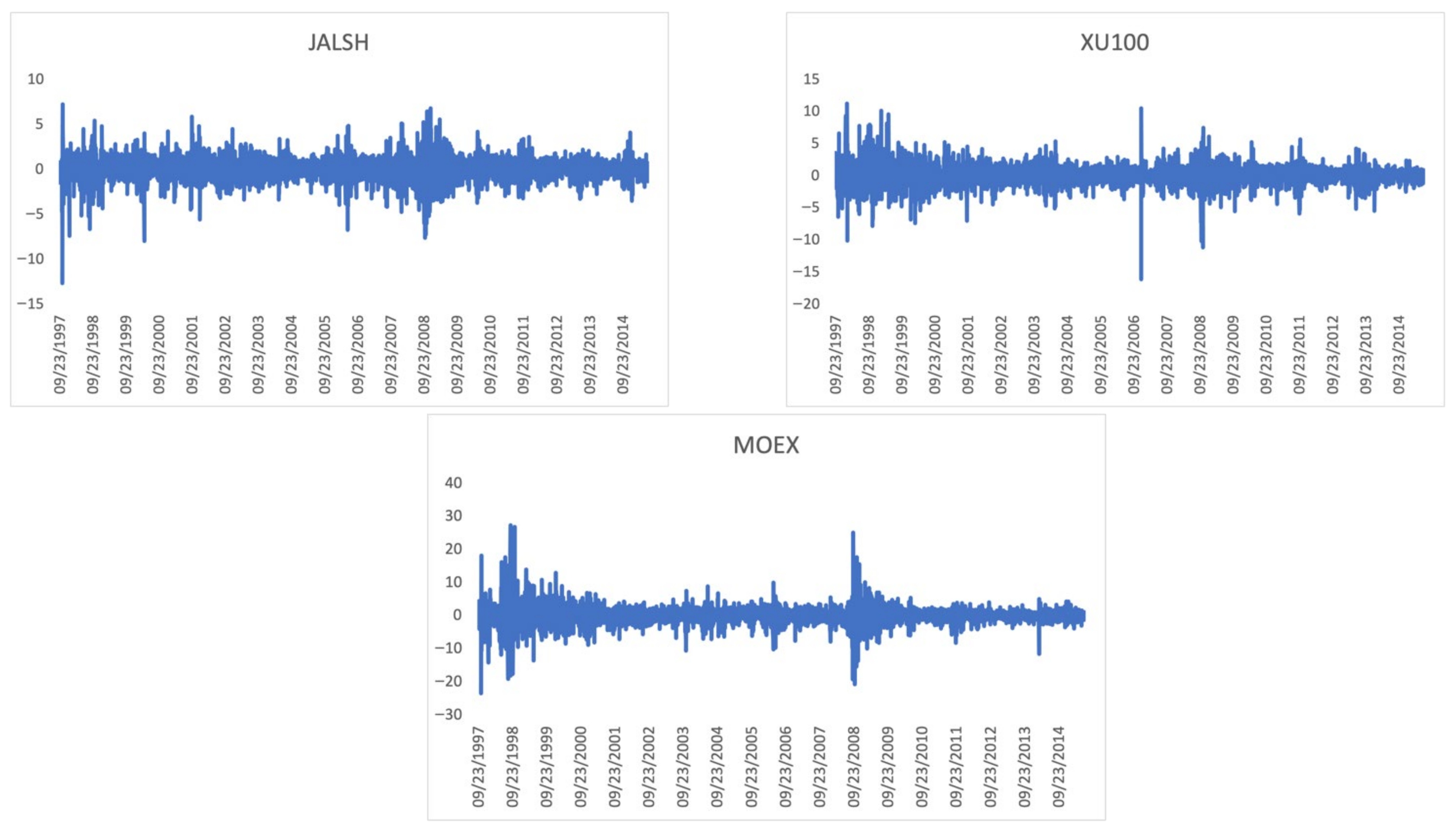
Figure 1 provides illustrations of each market’s returns over time for 1997–2015. We note that there were periods of excess volatility during our periods of interest (2007–2009) and around 2010. We also observe high volatility in the earlier years of the sample period. This could largely be due to the occurrence of the dot-com bubble, which impacted many markets once again. As the sample period chosen encompasses several crises, some of which this paper examines, we do observe some spikes in the market returns over the years. Moreover, we observe how volatile the markets are, with rapid increases and decreases (and significant highs and lows) over time.
Before proceeding with the necessary estimations, we convert the stock prices obtained using the following computation:
R t = l n p t p t 1 100
where returns at time t are denoted by R t , and p t and p t 1 represent the current and previous closing prices, respectively. Due to the fact that there are special events and holidays that result in missing observations, we make use of daily closing prices from the previous day in such instances.
Given that contagion analysis requires accurate selection of crisis and tranquil periods to identify idiosyncratic shocks, this paper makes use of the economic and statistical approaches to this end. Concerning the economic approach, we follow the Federal Reserve Bank of St. Louis (2009) and Kenourgios and Dimitriou (2015) to report the phases of the GFC. The breakdown of the phases related to the EDC are suggested by Kenourgios (2014) and Reuters (2020). These phases are reported in Table 2.
Furthermore, we follow the statistical approach to identify the phases of the two crises by employing the Markov switching dynamic regression (MS-DR) model. In a sense, by making use of the statistical approach, we further confirm and examine the robustness of the crisis period identification through the data. One could not stress enough the importance of the appropriate selection of crisis dates in studies related to contagion, which should render the results of the statistical analysis more reliable compared to other methods for random identification of crisis periods.
The following two-regime MS-DR model with varying intercepts and variances2 is estimated to identify crisis phases for the source countries, especially those related to the global financial crisis and the European debt crisis:
Regime   0 :   y t = v 0 + α 0 y t 1 + + x t β 0 + ϵ t ,   ϵ t ~ I I N 0 , σ 0 2
Regime   1 :   y t = v 1 + α 1 y t 1 + + x t β 1 + ϵ t ,   ϵ t ~ I I N 0 , σ 1 2
where x t is the control variable in the dynamic regression of y t . The probabilities of being in a regime can be written as follows:
P S t = 1 I t = 1 P ( S t = 0 | I t )
where I t contains all the information available up to time t such that I t = y t 1 , y t 2 , y t 3 ; x t .
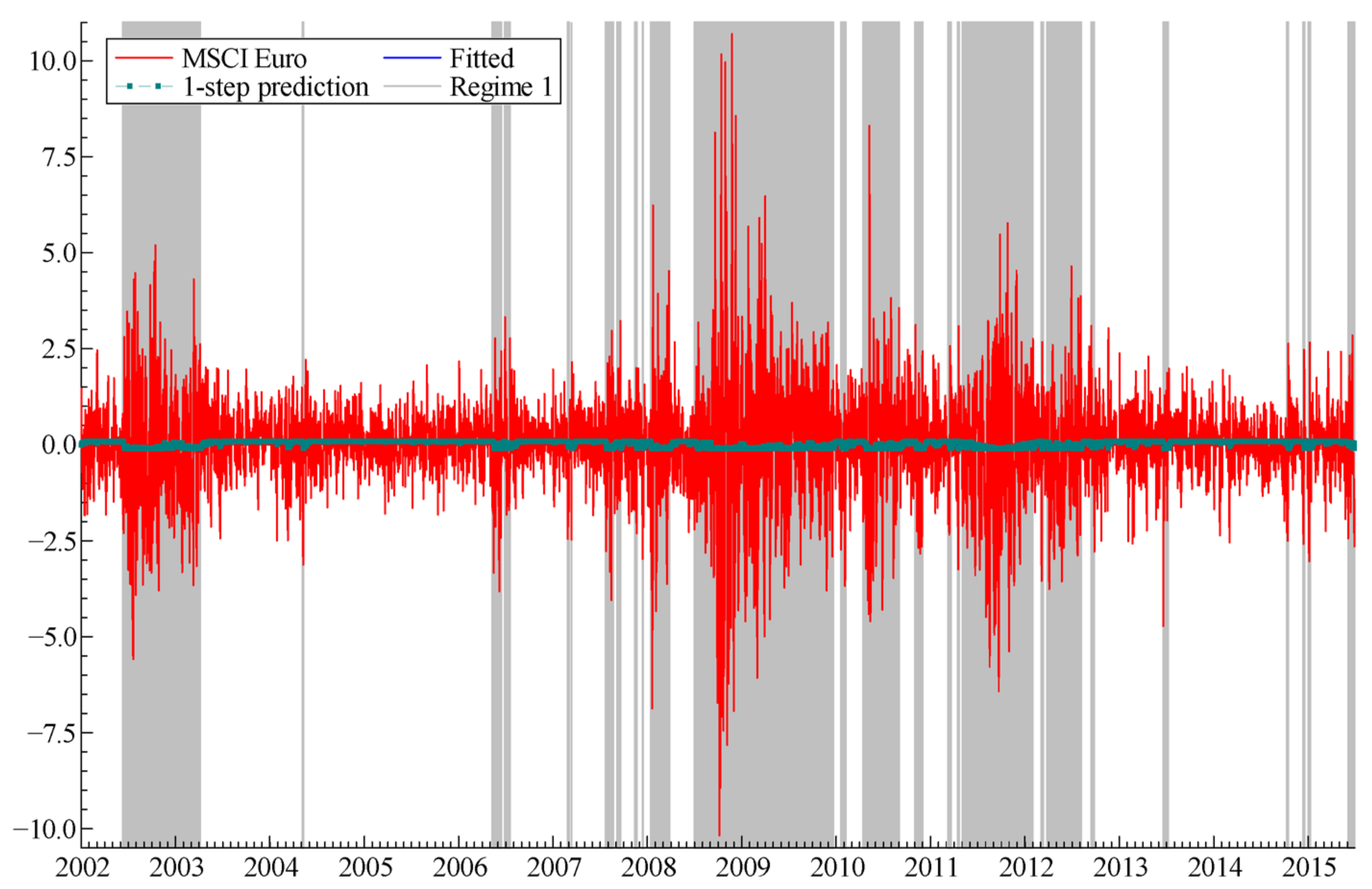
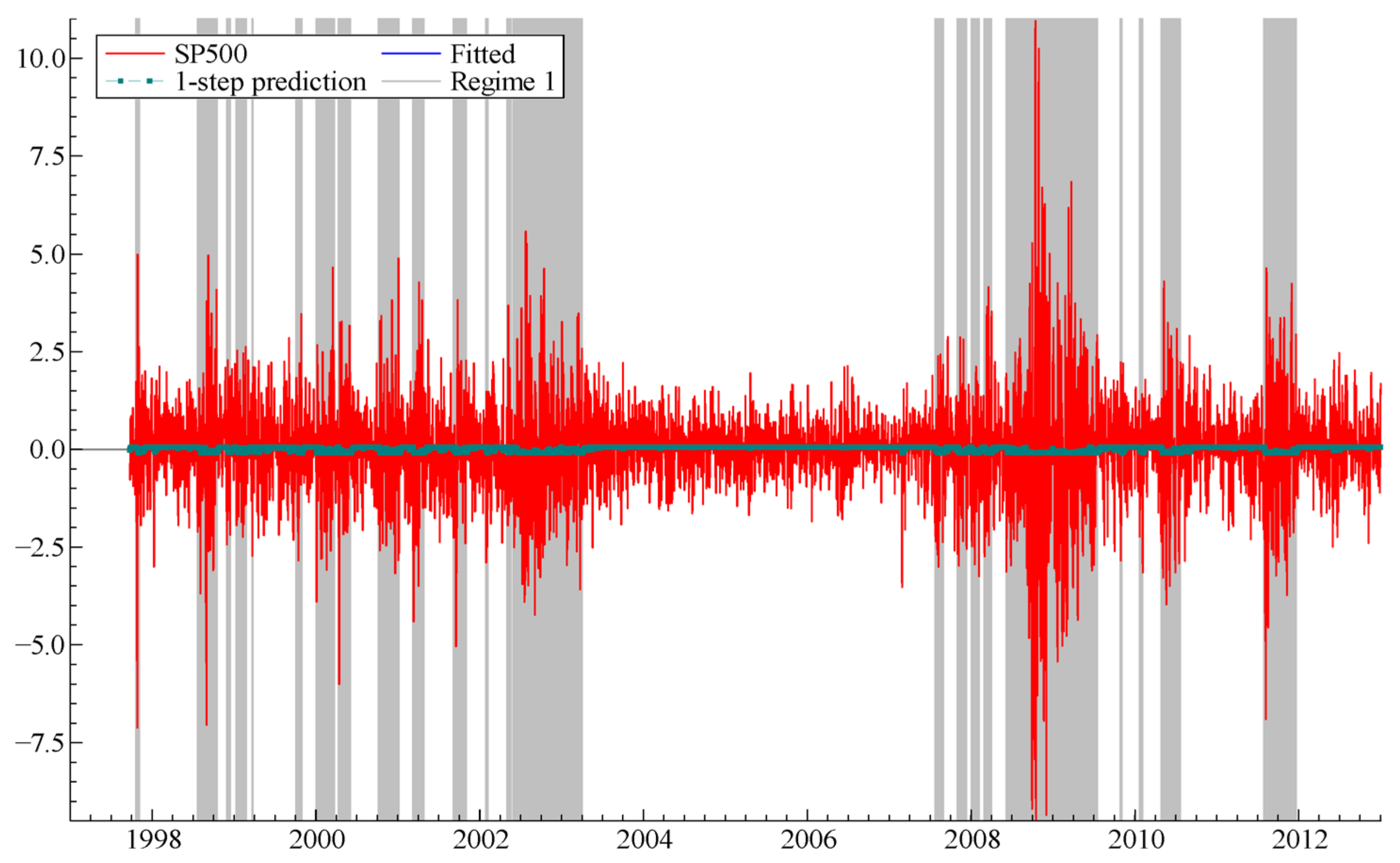
The periods of excess equity-market conditional volatilities identified by the MS-DR model make up regime 1 (the volatile regime) and thus identify the turmoil periods. Conversely, where low values of conditional volatilities are recorded, this is found to represent the tranquil periods, i.e., regime 0. The results are reported in Figure 2 and Figure 3 and summarized in Table 2 for the GFC and ESD crises.
The results reported in Table 2 show that while most of the dates pinpointed by the economic and statistical approaches overlap, the statistical approach identifies more phases related to excess volatility during the two crises. Henceforth, we conduct our analysis using the dates obtained through both approaches.

3.2. Estimations

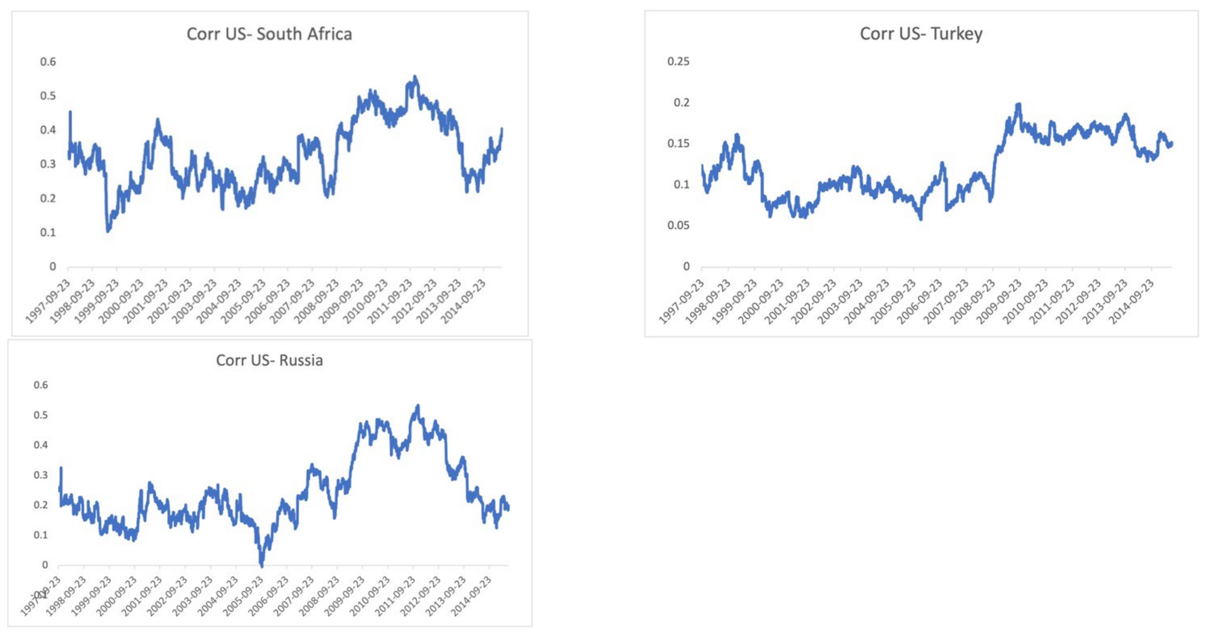
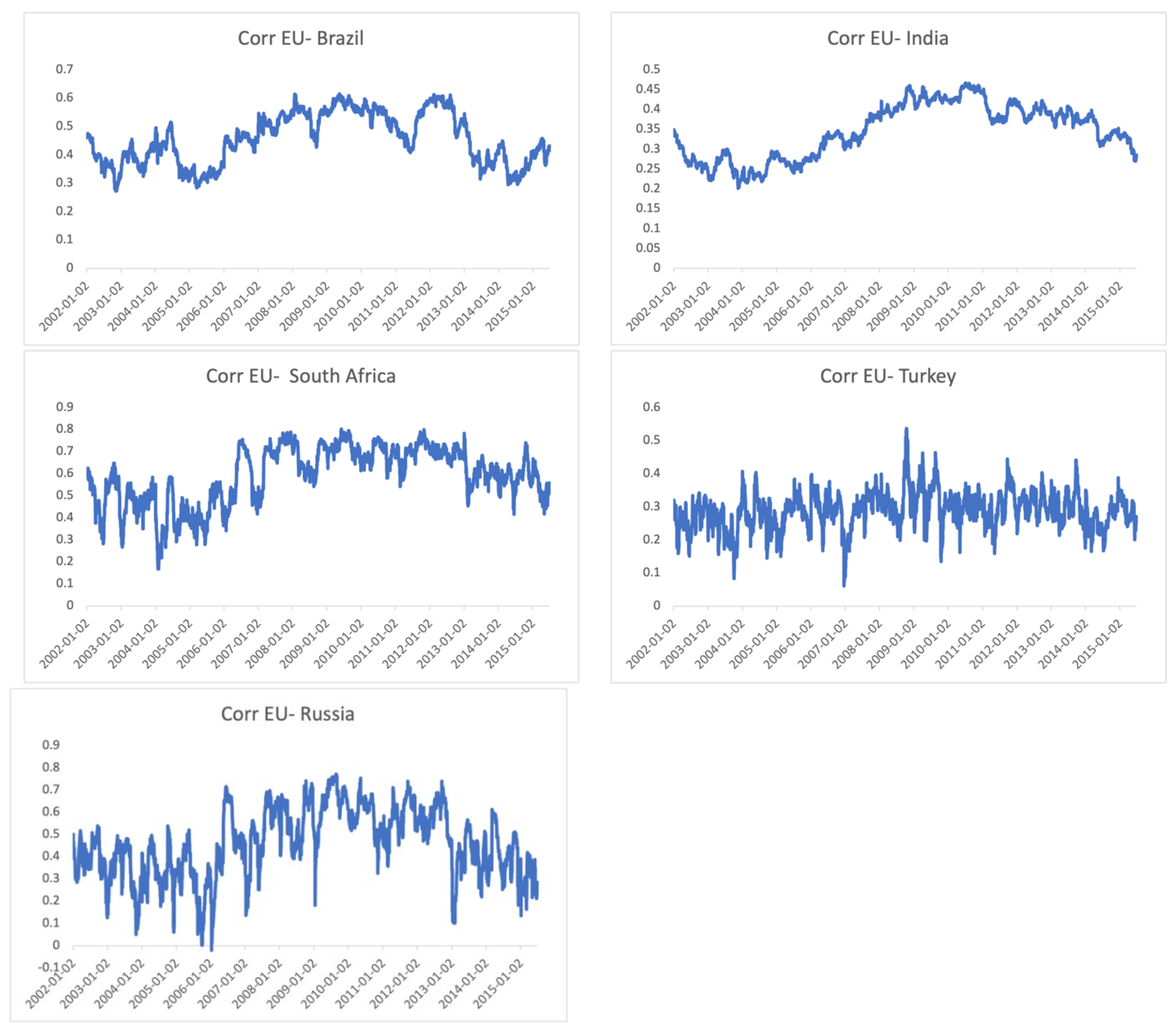
We follow the two-step procedure to estimate the A-DCC-GARCH model. In the first step, different GARCH models are applied for different countries informed by the AIC criteria. The A-DCC-GARCH model fits all the pair countries (US and EU with each of the emerging markets) for the estimation of their correlations3. Figure 4 and Figure 5 display the asymmetric dynamic correlations between the US and the EU with each of the emerging markets obtained from the estimated model.
The dynamic correlations displayed in Figure 4 and Figure 5 show high fluctuations during the two crises. For example, the dynamic correlation between the US and India shows a sharp structural break from 2008. The upward trend continued in the correlation between the two countries until the ESDC period. The same sharp changes are observed in the correlation between the US and Turkey. After a slight increase, the conditional correlation between the EU and Russia shows a significant decrease around the two crises. The decreasing trend may be attributed to the decoupling of Russia from the EU and US. However, such a conclusion can only be drawn after an empirical analysis.

3.3. Examination of Dynamic Conditional Correlations over Turmoil and Tranquil Periods

In order to assess whether there was contagion from the US and EU to emerging markets during the GFC and ESDC, we conduct the analysis at different levels. Firstly, we consider the entire sample related to each of the crises. Then, we conduct the analysis considering each of the phases identified from economic and statistical approaches, employing the suggested methodologies of entropy and regression tests. The entropy method tests the null hypothesis of the equality of density of the dynamic correlation between the US and EU with each of the emerging markets during the GFC and EDC, such as:
H 0 : f ( x ) C r i s i s = f ( y ) N o n   C r i s i s H 1 : f ( x ) C r i s i s f ( y ) N o n   C r i s i s
It is worth noting that the null hypothesis of the equality of density during the crisis and non-crisis periods refers to the concept of interdependence, i.e., markets are interdependent when the density functions of their dynamic correlations are equal during the crisis and non-crisis periods. The alternative hypothesis alludes to the differences between the density functions during the two periods, implying either contagion or decoupling. Once the alternative hypothesis is confirmed, a further test is needed to ensure whether decoupling or contagion occurs. The non-crisis period is selected to be the quiet period, either before or after the crisis period.
The results reported in Table 3 for the entire crisis periods of the GFC and ESDC show that the null hypothesis of equality of density function is rejected for all country pairs. This rejection implies no evidence of market interdependence between the US and EU and emerging markets. The rejection of the null hypothesis supports the alternative hypothesis that there was either contagion or decoupling between these countries during the mentioned crisis periods. Thus, a further test is needed to ascertain whether contagion or decoupling occurred.
It is worth noting that tests based on regression analysis need to identify dummy variables corresponding to the relevant crises. The regression analysis is based on the following model:
ρ t = α + c 1 D M t   G F C + c 2 E R , t + c 3 I R D t + ε t
ρ t = α + c 1 D M t   E S D C + c 2 E R t + c 3 I R D , t + ε t
where ρ t represents the correlation between the source market “US or EU” and response market “each emerging market”, α represents the constant term, and DM denotes the dummy variables corresponding to the relevant crises. We make use of control variables E R , t and I R D t , the exchange rate and interest rate differentials between the two markets, respectively (see Hwang et al. (2013) and Pretorius (2002)).
Table 4 and Table 5 present the results obtained for the GFC and ESDC, without accounting for related phases, following the estimation of Equations (4) and (5). The results show the existence of contagion effects between the market pairs, except in the case of US–Russia, where the Russian stock market appears to have insulated from the US during the GFC, with a statistically significant DMGFC coefficient of −0.04989 showing that the correlation between the US and Russia declined during the GFC compared to the tranquil period. This finding is supported by the observation on the conditional correlation graph in Figure 4, where the correlation between the US and Russia declined for some parts of the GFC period. The possible decoupling of Russia from the US during the GFC may be supported by Russia being a big resource-endowed country. Some of these resources play the role of safe-haven investment and provide a cushion against financial crises (see Sutela 2010).
Contrary to the US–Russia outcome that supports decoupling, we find strong evidence of the contagion phenomenon in the remaining market pairs, such as between the US and Brazil, India, South Africa, and Turkey.
Although Russia is found to be insulated from the US subprime crisis, the same cannot be said with the ESDC, as per the results reported in Table 5. The evidence of contagion between Russia and the EU, as reported in Table 5, may be due to Russia’s different interrelationships with the EU. For example, the better trade relationship Russia has with the EU compared to the US would partially explain why Russia’s markets were more vulnerable to shocks originating from the EU. Moreover, Table 5 shows that most of the emerging markets considered were affected by the ESDC-related spillover effects, except for Turkey. The pair’s dummy coefficient is insignificant for EU–Turkey, suggesting that the Turkish market decoupled or insulated from the EU during the crisis.
The above findings did not account for the different phases during the two crises. This oversight may cast doubt on the validity of the findings discussed above, as the GFC and ESDC had distinct stages, each with varying externalities. As a result, we find it essential to further analyze the crises in phases in addition to the entire crisis period analysis, where we use both the economic and statistical approaches obtained in the subperiods. Studies that only rely on the economic approach do not consider what the actual data tell us about that period. Since the statistical approach relies on the data, we believe that results obtained from the economic approach alone, without accounting for endogenously detected crisis regimes or phases, can be misleading. Thus, we proceed with a combination of both approaches.
Table 6 presents the entropy test results related to phases derived from the economic approach. Just like in the aggregated crises reported in Table 4 and Table 5, the results reported in Table 6 reject the null hypothesis of interdependence in all the phases related to the GFC and ESDC. We accept the alternative hypothesis of contagion or decoupling. We then proceed with the regression analysis and report the results in Table 7 and Table 8 for the GFC and ESDC, respectively.
Concerning Table 7, the dummy coefficient for the US–Brazil pair is not statistically different to zero during phase 1. This result entails that Brazil was insulated or decoupled from the GFC during phase 1. Similar findings are obtained in the case of Turkey and South Africa, supporting the decoupling hypothesis for these countries. The positive and significant coefficient for Russia and India is strong evidence of contagion effects during phase 1 of the GFC. This contagion seems short-lived for Russia, as the country later decoupled from the US in the remaining phases of the deepening global financial crisis. India continued to feel the full brunt of the spillover effects from the US market in the final stage, with a positive and significant coefficient. India insulated from the US during phase 2. On the other hand, Brazil, South Africa, and Turkey exhibited contagion effects in phases 2 and 3, as the positive and significant coefficients indicated that the correlation increased during the subperiods compared to the tranquil periods. Phase 2, characterized by sharp financial market deterioration, was detrimental for all equity markets except India and Russia.
Compared to the GFC, emerging markets have been more vulnerable to shocks from the EU during the ESDC, with more evidence of contagion effects established. Table 8 reports positive and significant dummy coefficients for the EU and Brazil, India, South Africa, and Russia market pairs during all three phases. We observe that during the different stages of the crisis, correlations increased between the markets compared to the periods of tranquility. Thus, we conclude in support of the presence of contagion effects. On the contrary, the results found in the case of the EU–Turkey market pair support the decoupling hypothesis during phases 1 and 2 of the ESDC.
Following the statistical approach, the results reported in Table 9 show that the null hypothesis of the equality of distributions between the crisis and non-crisis periods is rejected for the GFC and ESDC, supporting the alternative hypothesis of either contagion or decoupling. We proceed to regression analysis to determine whether there was contagion or decoupling.
The results in Table 10 show the contagion between the US and India in all the phases. The same can be said for the first two phases of the GFC in the case of US–Brazil, the first three phases for US–Russia, and the last for US–Turkey. However, during phases 3 and 4 of the global financial crisis, Brazil and South Africa had negative coefficients of the related dummy variables. Turkey and Russia completely insulated and decoupled from the US market during phases 4 and 5.
In the case of the ESDC, the results displayed in Table 11 indicate that although the contagion hypothesis is dominant for most of the phases, there is evidence of decoupling during phase 3 for the Brazil, Russia, and Turkey markets and phase 2 for Turkey.
The findings reported in this paper show that emerging markets intertwined episodes or phases of contagion and decoupling during the two very significant economic and financial crises originating from the US and Europe. While there have been controversial findings in past studies on whether emerging markets truly decoupled from developed economies, this paper suggests that this controversy may be due to the failure of these studies to disaggregate the phases of these crises and apply appropriate tests that account for the density of the distribution rather than a few moments of the distribution. On the importance of identifying the actual phases of the crisis, the aggregate analysis of the GFC shows that Russia completely decoupled from the GFC. However, when we disaggregated the GFC by accounting for the different phases, the findings of the paper show that the Russian economy decoupled from the GFC only during specific phases, but not the full GFC. Moreover, all emerging economies decoupled from the GFC at least in one of the phases, contrary to the aggregate analysis results.
It is worth noting that the decoupling of most emerging economies may be due mainly to their resource endowment. Studies show that resource-dependent nations performed slightly better than others during the crisis (Gaddy and Ickes 2010; Mensi et al. 2016). We postulate that countries that produce commodities that serve as safe havens during economic and financial crises, such as gold, stand the chance to insulate themselves from contagion during global crises.
India was the hardest-hit emerging country in the two crises. Based on the statistical approach, India was adversely impacted in all five phases of the GFC, while the economic approach saw the country weather the storm only in phase 2. Nonetheless, we find India to have been the hardest-affected market in the study during the GFC. Joseph (2009) shows that the country experienced an “abrupt stop” in capital inflows and a slump in both domestic and external demand during the GFC. Most importantly, India is not an abundantly resourced country compared to Russia, for example.
It is important to note that contagion can still take place in resource-endowed countries, although to a lesser extent if these countries have a significant trade linkage with the crisis-originating countries. For example, while Russia seemed to fare well during the GFC, the country was far from immune during some phases of the ESDC. This outcome could be explained by the increasing dependency of Russia on EU demand, especially for energy commodities and raw materials (see Tajoli 2022; Khrushcheva and Maltby 2016).
The results obtained in this paper should be of interest to investors and asset or portfolio managers, as they shed more light on portfolio diversification. Our findings suggest that many emerging markets provide asset diversification options for many developed economies, such as the US and EU, during periods of downside risks. Studies show that during periods of economic downturns or recession in developed countries such as the United States, investors often seek out alternative investment opportunities that are less affected by the downturn (see Zhang 2016). In recent years, many investors have turned to emerging markets, such as the BRICS countries, as a source of diversification due to their strong economic growth and large populations. For example, during the 2008 global financial crisis, many investors sought out investments in the BRICS countries as a way to diversify their portfolios and reduce their exposure to the US and European markets. This was because the BRICS countries were less affected by the crisis due to their less developed financial systems and less exposure to the US subprime mortgage market (see Naresh et al. 2018; Mensi et al. 2017). Furthermore, the decoupling of Russia from the US, and to a lesser extent the EU, should provide insight to policymakers worldwide who intend to impose sanctions on Russia due to the Ukraine war. In the event that Russia successfully diverts trade from the EU, it may be able to decouple the country from the EU and become immune from any sanctions it might face.

4. Conclusions

This paper proposes a test based on entropy theory to distinguish between the interdependence, decoupling, and contagion hypotheses when assessing shock spillovers between countries or regions. We apply the theory and methodology to test the nature of shock spillovers between advanced economies, the US and the EU, and emerging markets in different regions during the GFC and ESDC. In doing so, we assessed whether emerging markets are homogeneous or heterogeneous as recipients of shock spillovers from advanced economies. Another significant contribution of this study is distinguishing between the phases of each crisis based on an economic and statistical framework. Studies show that accurately identifying crisis episodes is essential when determining the extent of contagion or interdependence between markets or countries (see Baur 2012; Dimitriou et al. 2013; Kenourgios et al. 2016). Results of the empirical analysis indicate that it is vital to test these three hypotheses in the context of phases or episodes of these crises instead of using aggregate analyses. The results show that while most emerging markets were decoupled from the two advanced countries during some specific phases of the GFC and ESDC, Russia seems the most decoupled country from the crises emanating from the US and EU. Moreover, the results allude to the importance of a density test and the significance of assessing the three hypotheses accounting for the different stages of financial and economic crises. Further studies can apply the methodology to other major crises. Moreover, the findings of this paper can inform and should help policymakers and investors to conduct phase-specific analyses (rather than aggregate assessments) to identify optimal diversification windows.

Author Contributions

Conceptualization, L.B.-B. and Z.L.N.; methodology, L.B.-B. and Z.L.N.; software, L.B.-B.; validation, L.B.-B. and Z.L.N.; formal analysis, L.B.-B. and zinzile ndiweni; investigation, L.B.-B.; resources, L.B.-B.; data curation, L.B.-B.; writing—original draft preparation, L.B.-B. and Z.L.N.; writing—review and editing, L.B.-B. and Z.L.N.; visualization, L.B.-B.; supervision, L.B.-B.; project administration, L.B.-B. All authors have read and agreed to the published version of the manuscript.

Funding

This research received no external funding.

Data Availability Statement

The raw data supporting the conclusions of this article will be made available by the authors on request.

Conflicts of Interest

The authors declare no conflict of interest.

Notes

1
Although the latest observations are available, they are not important in the context of this paper.
2
The model accounts for the change in the mean and volatility in the two regimes. Lag order and number of states selected according to AIC.
3
Their parameter estimations can be provided on request.

References

  1. Acatrinei, Mădălina, Alexandru Gorun, and Nicolae Marcu. 2013. A DCC-GARCH Model to Estimate. Romanian Journal of Economic Forecasting 1: 136–48. [Google Scholar]
  2. Altun, Ali A., Sıtkı Çelik, and Yusuf D. Koç. 2019. Testing for Financial Contagion: New Evidence from the European Debt Crisis. Panoeconomicus 66: 611–32. [Google Scholar] [CrossRef]
  3. Bannigidadmath, Deepak, and Paresh Kumar Narayan. 2016. Stock Return Predictability and Determinants of Predictability and Profits. Emerging Markets Review 26: 153–73. [Google Scholar] [CrossRef]
  4. Baur, Dirk G. 2012. Financial Contagion and the Real Economy. Journal of Banking & Finance 36: 2680–92. [Google Scholar] [CrossRef]
  5. Baur, Dirk G. 2020. Decoupling and Contagion: The Special Case of the Eurozone Sovereign Debt Crisis. International Review of Finance 20: 133–54. [Google Scholar] [CrossRef]
  6. Bekiros, Stelios D. 2014. Contagion, Decoupling and the Spillover Effects of the US Financial Crisis: Evidence from the BRIC Markets. International Review of Financial Analysis 33: 58–69. [Google Scholar] [CrossRef]
  7. Benkraiem, Ramzi, Faouzi Lakhal, Ramzi Garfatta, and Imen Zorgati. 2022. Financial Contagion Intensity during the COVID-19 Outbreak: A Copula Approach. International Review of Financial Analysis 81: 102136. [Google Scholar] [CrossRef]
  8. Bonga-Bonga, Lumengo. 2018. Uncovering Equity Market Contagion among BRICS Countries: An Application of the Multivariate GARCH Model. The Quarterly Review of Economics and Finance 67: 36–44. [Google Scholar] [CrossRef]
  9. Bonga-Bonga, Lumengo, and Mthokozisi M. Manguzvane. 2020. Assessing the Extent of Contagion of Sovereign Credit Risk among BRICS Countries. Economics Bulletin 40: 1017–32. [Google Scholar]
  10. Cappiello, Lorenzo, Robert F. Engle, and Kevin Sheppard. 2006. Asymmetric Dynamics in the Correlations of Global Equity and Bond Returns. Journal of Financial Econometrics 4: 537–72. [Google Scholar] [CrossRef]
  11. Chittedi, Krishna Reddy. 2015. Financial Crisis and Contagion Effects to Indian Stock Market: DCC–GARCH Analysis. Global Business Review 16: 50–60. [Google Scholar] [CrossRef]
  12. Cho, Jin Hyuk, and Ali M. Parhizgari. 2009. East Asian Financial Contagion under DCC-GARCH. International Journal of Banking and Finance 6: 17–30. [Google Scholar] [CrossRef]
  13. Corbet, Shaen, Yifan Hu, Yifan Hou, and Les Oxley. 2022. Financial Contagion among COVID-19 Concept-Related Stocks in China. Applied Economics 54: 2439–52. [Google Scholar] [CrossRef]
  14. Cuadro-Sáez, Luis, Marcel Fratzscher, and Christian Thimann. 2009. The Transmission of Emerging Market Shocks to Global Equity Markets. Journal of Empirical Finance 16: 2–17. [Google Scholar] [CrossRef]
  15. Çelik, Sıtkı. 2012. The More Contagion Effect on Emerging Markets: The Evidence of DCC-GARCH Model. Economic Modelling 29: 1946–59. [Google Scholar] [CrossRef]
  16. Dimitriou, Dimitrios, Dimitrios Kenourgios, and Theodore Simos. 2013. Global Financial Crisis and Emerging Stock Market Contagion: A Multivariate FIAPARCH–DCC Approach. International Review of Financial Analysis 30: 46–56. [Google Scholar] [CrossRef]
  17. Dungey, Mardi, and Dharma Gajurel. 2014. Equity Market Contagion during the Global Financial Crisis: Evidence from the World’s Eight Largest Economies. Economic Systems 38: 161–77. [Google Scholar] [CrossRef]
  18. Eichengreen, Barry, Andrew K. Rose, and Charles Wyplosz. 1996. Contagious Currency Crises. NBER Working Paper 5681. Cambridge: National Bureau of Economic Research. [Google Scholar]
  19. Federal Reserve Bank of St. Louis. 2009. The Financial Crisis: A Timeline of Events and Policy Actions. St. Louis: Federal Reserve Bank of St. Louis. [Google Scholar]
  20. Fernández, Andrés, Stephanie Schmitt-Grohé, and Martín Uribe. 2017. World Shocks, World Prices, and Business Cycles: An Empirical Investigation. Journal of International Economics 108, (Suppl. 1): S2–S14. [Google Scholar]
  21. Forbes, Kristin J., and Roberto Rigobon. 2002. No Contagion, Only Interdependence: Measuring Stock Market Comovements. The Journal of Finance 57: 2223–61. [Google Scholar] [CrossRef]
  22. Gaddy, Clifford G., and Barry W. Ickes. 2010. Russia after the Global Financial Crisis. Eurasian Geography and Economics 51: 281–311. [Google Scholar] [CrossRef]
  23. Hamao, Yasushi, Ronald W. Masulis, and Victor Ng. 1990. Correlations in Price Changes and Volatility across International Stock Markets. Review of Financial Studies 3: 281–307. [Google Scholar] [CrossRef]
  24. Hemche, Omar, Sofiane B. Maliki, Frédéric Jawadi, and Abderrazak I. Cheffou. 2016. On the Study of Contagion in the Context of the Subprime Crisis: A Dynamic Conditional Correlation–Multivariate GARCH Approach. Economic Modelling 52: 292–99. [Google Scholar] [CrossRef]
  25. Hwang, Eui Jung, Byung Hee Kim, Hyung-Geun Min, and Hail Kim. 2013. Determinants of Stock Market Comovements among US and Emerging Economies during the US Financial Crisis. Economic Modelling 35: 338–48. [Google Scholar] [CrossRef]
  26. Joseph, Mathew. 2009. Global Financial Crisis: How Was India Impacted. Paper presented at InWEnt-DIE Conference on Global Financial Governance—Challenges and Regional Responses, Vienna, Austria, September 3–4. [Google Scholar]
  27. Kenourgios, Dimitrios. 2014. On Financial Contagion and Implied Market Volatility. International Review of Financial Analysis 34: 21–30. [Google Scholar] [CrossRef]
  28. Kenourgios, Dimitrios, and Dimitrios Dimitriou. 2015. Contagion of the Global Financial Crisis and the Real Economy: A Regional Analysis. Economic Modelling 44: 283–93. [Google Scholar] [CrossRef]
  29. Kenourgios, Dimitrios, Nidhaleddine Naifar, and Dimitrios Dimitriou. 2016. Islamic Financial Markets and Global Crises: Contagion or Decoupling? Economic Modelling 57: 36–46. [Google Scholar] [CrossRef]
  30. Khrushcheva, Olga, and Tomas Maltby. 2016. The Future of EU-Russia Energy Relations in the Context of Decarbonisation. Geopolitics 21: 799–830. [Google Scholar] [CrossRef]
  31. Lawlor, Philip. 2020. Not All Emerging Markets Are Equal: Tread Carefully When Chasing Returns. Investec. Available online: https://www.investec.com/en_za/focus/global-investment-strategy-group/not-all-emerging-markets-are-equal-tread-carefully-when-chasing-returns.html (accessed on 26 April 2025).
  32. Li, Qi, Esfandiar Maasoumi, and Jeffrey S. Racine. 2009. A Nonparametric Test for Equality of Distributions with Mixed Categorical and Continuous Data. Journal of Econometrics 148: 186–200. [Google Scholar] [CrossRef]
  33. Mensi, Walid, Duc Khuong Nguyen, Shawkat Hammoudeh, and Seungho H. Kang. 2016. Global Financial Crisis and Spillover Effects among the US and BRICS Stock Markets. International Review of Economics & Finance 42: 257–76. [Google Scholar] [CrossRef]
  34. Mensi, Walid, Syed Jawad Hussain Shahzad, Shawkat Hammoudeh, Rami Zeitun, and Muhammad Umer Rehman. 2017. Diversification potential of Asian frontier, BRIC emerging and major developed stock markets: A wavelet-based value at risk approach. Emerging Markets Review 32: 130–47. [Google Scholar] [CrossRef]
  35. Naoui, Khaled, Sami Khemiri, and Nabil Liouane. 2010. Crises and financial contagion: The subprime crisis. Journal of Business Studies Quarterly 2: 15. [Google Scholar]
  36. Narayan, Paresh Kumar, and Susan Sunila Sharma. 2015. Does data frequency matter for the impact of forward premium on spot exchange rate? International Review of Financial Analysis 39: 45–53. [Google Scholar] [CrossRef]
  37. Naresh, Gokul, Ganesh Vasudevan, Subramaniam Mahalakshmi, and S. Thiyagarajan. 2018. Spillover effect of US dollar on the stock indices of BRICS. Research in International Business and Finance 44: 359–68. [Google Scholar] [CrossRef]
  38. Pretorius, Elna. 2002. Economic determinants of emerging stock market interdependence. Emerging Markets Review 3: 84–105. [Google Scholar] [CrossRef]
  39. Reuters. 2020. Pandemic Won’t Cause Euro Debt Crisis, but a North-South Divide. Available online: https://www.reuters.com/article/us-health-coronavirus-eu-debt-analysis-idUSKCN2240N6 (accessed on 24 April 2025).
  40. Rigobon, Roberto. 2002. International Financial Contagion: Theory and Evidence in Evolution. Charlottesville: Research Foundation of AIMR. [Google Scholar]
  41. Soylu, Pelin Kizilkaya, and Bülent Güloğlu. 2019. Financial contagion and flight to quality between emerging markets and US bond market. The North American Journal of Economics and Finance 50: 100992. [Google Scholar] [CrossRef]
  42. Sutela, Pekka. 2010. Russia’s Response to the Global Financial Crisis. Available online: http://carnegieendowment.org (accessed on 24 April 2025).
  43. Tajoli, Lucia. 2022. Too much of a good thing? Russia-EU international trade relations at times of war. Journal of Industrial and Business Economics 49: 807–34. [Google Scholar] [CrossRef]
  44. Wälti, Sébastien. 2012. The myth of decoupling. Applied Economics 44: 3407–19. [Google Scholar] [CrossRef]
  45. Willett, Thomas D., Ping Liang, and Nan Zhang. 2011. Global contagion and the decoupling debate. In The Evolving Role of Asia in Global Finance. Edited by Yin-Wong Cheung, Vikas Kakkar and Guonan Ma. Bingley: Emerald Group Publishing Limited, pp. 215–34. [Google Scholar] [CrossRef]
  46. Zhang, Yan. 2016. Emerging markets and international asset allocation. Journal of International Financial Markets, Institutions and Money 44: 56–80. [Google Scholar]
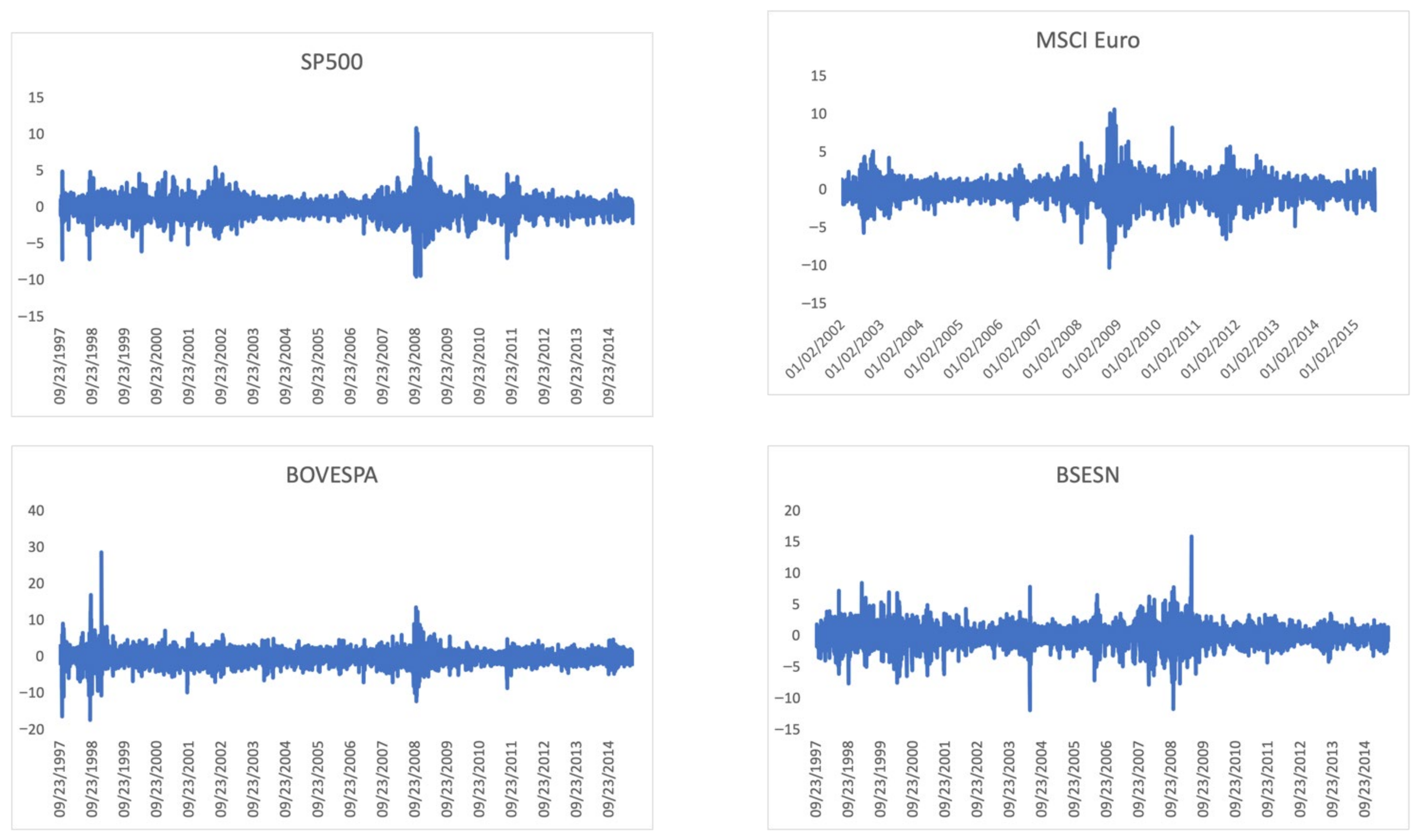
Figure 1. Stock market returns over time (1997–2015). Source: authors’ calculations.
Risks 13 00165 g001aRisks 13 00165 g001b
Figure 2. Actual data and estimated high-volatility regime (regime1) for Europe. Source: authors’ calculations. Note: The gray-shaded areas represent the regimes of excess volatilities identified by the MS-DR model, while the red represents the volatilities.
Risks 13 00165 g002
Figure 3. Actual data and estimated high-volatility regime (regime 1) for SP500. Source: authors’ calculations. Note: The grey-shaded areas represent the regimes of excess volatilities identified by the MS-DR model, while the red represents the conditional volatilities.
Risks 13 00165 g003
Figure 4. Asymmetric dynamic correlations between the US and the emerging markets over time. Source: authors’ calculations.
Risks 13 00165 g004aRisks 13 00165 g004b
Figure 5. Asymmetric dynamic correlations between the EU and the emerging markets over time. Source: authors’ calculations.
Risks 13 00165 g005
Table 1. Variables and classification.
VariableClassification
S&P 500 (US)
MSCI Europe Index (EU)
Source market (developed)
BOVESPA (Brazil)Recipient market (Latin American emerging market)
BSESN (India)Recipient market (Asian emerging market)
JALSH (South Africa)Recipient market (African emerging market)
XU100 (Turkey)Recipient market (Middle East emerging market)
MOEX (Russia)Recipient market (European emerging market)
Table 2. GFC and ESDC phases.
GFCESDC
Entire crisis periodAugust 2007–March 2009November 2009–July 2012
Phases (economic approach)
Phase 11 Aug 2007–15 Sept 2008 (dubbed “initial financial turmoil”)5 November 2009–22 April 2010 (announcement of Greek budget deficit)
Phase 216 Sept 2008–31 Dec 2008 (defined as “sharp financial market deterioration”)23 April 2010–14 July 2011 (announcement that the austerity packages were not enough and request for bailout from IMF or EU)
Phase 31 Jan 2009–31 Mar 2009
(dubbed “macroeconomic deterioration”)
15 July 2011–onwards
(begins when banking stress tests were published by the European authorities and the first austerity package was announced by Italy)
Phase 41 Apr 2009–30 Nov 2009 (described as a phase of “stabilization and tentative signs of recovery”)
Phases (statistical approach)
Phase 124 Jul 2007–29 Aug 200719 Jan 2010–8 Feb 2010
Phase 231 Oct 2007–11 Nov 200716 Apr 2010–2 Sept 2010
Phase 32 Jan 2008–6 Feb 20082 Nov 2010–3 Dec 2010
Phase 428 Feb 2008–1 Apr 200831 May 2011–1 Feb 2012
Phase 55 Jun 2008–16 Jul 200926 Mar 2012–6 Aug 2012
Sources: published news, reliable sources (economic approach) and authors’ calculations (statistical approach).
Table 3. Entropy test statistics (entire crisis periods for GFC and ESDC).
Test Statistic Spp-ValueOutcome
US–Brazil0.19924222.22 × 10−16 *** H 0 rejected
US–India0.19886452.22 × 10−16 *** H 0 rejected
US–South Africa0.19924220.000000 *** H 0 rejected
US–Turkey0.19895482.22 × 10−16 *** H 0 rejected
US–Russia0.1965120.000000 *** H 0 rejected
EU–Brazil0.22134910.000000 *** H 0 rejected
EU–India0.19246232.22 × 10−16 *** H 0 rejected
EU–South Africa0.17597792.22 × 10−16 *** H 0 rejected
EU–Turkey0.21125580.000000 *** H 0 rejected
EU–Russia0.2066112.22 × 10−16 *** H 0 rejected
Source: authors’ calculations. Note: *** denote rejection of the null hypothesis of equality at 1% levels.
Table 4. GFC regression analysis (entire crisis period).
US–BrazilUS–IndiaUS–South AfricaUS–TurkeyUS–Russia
α 0 0.75749053
(0.000000) ***
−0.1710778
(8.591 × 10⁻³⁴) ***
0.2054267
(6.547 × 10−260) ***
0.09508578
(1.385 × 10−297) ***
0.30636772
(1.1311 × 10⁻¹⁶) ***
DMGFC0.05059396
(2.7437 × 10⁻¹⁹) ***
0.02990513
(2.101 × 10⁻¹⁹) ***
0.03847949
(7.09 × 10⁻³²) ***
0.00841855
(5.1556 × 10−05) ***
−0.0498957
(5.159 × 10⁻¹⁰) ***
Exchange rate−0.0394569
(5.2727 × 10−36) ***
0.00644579
(3.4417 × 10−88) ***
0.00729892
(3.4535 × 10⁻²³) ***
0.02187474
(5.3031 × 10−44) ***
−0.0020963
(0.09748546) *
Interest rate differential0.00622531
(1.117 × 10−104) ***
−0.0058543
(3.5853 × 10−62) ***
−0.0017017
(8.6098 × 10−08) ***
0.00015832
(5.1981 × 10⁻¹⁵) ***
−0.018169
(8 × 10−147) ***
SE0.1076980.062884460.098712510.040469410.11757167
p-value6.99 × 10−2065.103 × 10−2321.0375 × 10−771.17 × 10−1050.000000
Source: authors’ calculations. Note: *** and * denote rejection of the null hypothesis of equality at 1% and 10% levels.
Table 5. ESDC regression analysis (entire crisis period).
EU–BrazilEU–IndiaEU–South AfricaEU–TurkeyEU–Russia
α 0 0.6492135
(0.000000) ***
0.10892246
(5.3771 × 10−69) ***
0.29577398
(5.951 × 10−138) ***
0.32615524
(0.000000) ***
0.6015557
(3.024 × 10−202) ***
DMESDC0.05934492
(1.9945 × 10−67) ***
0.08429326
(6.412 × 10−276) ***
0.14149668
(5.226 × 10−189) ***
0.00446084
(0.06973659) *
0.1567137
(4.708 × 10−143) ***
Exchange rate−0.0325584
(3.0311 × 10⁻²¹) ***
0.00377976
(1.043 × 10−211) ***
0.02633883
(2.519 × 10−176) ***
−0.0088868
(0.00108001) ***
−0.005272
(9.4971 × 10⁻²⁴) ***
Interest rate differential0.00948557
(1.466 × 10−156) ***
0.00335053
(4.0995 × 10⁻¹⁶) ***
0.00127841
(0.19180879)
0.00139337
(2.2256 × 10−36) ***
−0.0105106
(3.1155 × 10⁻³³) ***
SE0.066440350.04954120.105333720.054748490.13964641
p-value0.0000000.0000000.0000005.2451 × 10−514.003 × 10−167
Source: authors’ calculations. Note: *** and * denote rejection of the null hypothesis of equality at 1% and 10% levels.
Table 6. Entropy test results (economic approach).
Test Statistic Spp-Value Outcome
US–BrazilPhase 1
Phase 2
Phase 3
0.2034821
0.1954202
0.2101099
2.22 × 10⁻¹⁶ ***
2.22 × 10⁻¹⁶ ***
0.000000 ***
H 0 rejected
H 0 rejected
H 0 rejected
US–IndiaPhase 1
Phase 2
Phase 3
0.1925159
0.2054686
0.1801679
2.22 × 10⁻¹⁶ ***
0.000000 ***
2.22 × 10⁻¹⁶ ***
H 0 rejected
H 0 rejected
H 0 rejected
US–South AfricaPhase 1
Phase 2
Phase 3
0.2178756
0.178754
0.2200741
0.000000 ***
2.22 × 10⁻¹⁶ ***
2.22 × 10⁻¹⁶ ***
H 0 rejected
H 0 rejected
H 0 rejected
US–TurkeyPhase 1
Phase 2
Phase 3
0.2052791
0.2162047
0.2041979
2.22 × 10⁻¹⁶ ***
0.000000 ***
2.22 × 10⁻¹⁶ ***
H 0 rejected
H 0 rejected
H 0 rejected
US–Russia Phase 1
Phase 2
Phase 3
0.2103451
0.20185
0.1870066
0.000000 ***
2.22 × 10⁻¹⁶ ***
0.000000 ***
H 0 rejected
H 0 rejected
H 0 rejected
EU–BrazilPhase 1
Phase 2
Phase 3
0.2013982
0.2024698
0.1925159
0.000000 ***
2.22 × 10⁻¹⁶ ***
2.22 × 10⁻¹⁶ ***
H 0 rejected
H 0 rejected
H 0 rejected
EU–IndiaPhase 1
Phase 2
Phase 3
0.201031
0.1881834
0.1989455
2.22 × 10⁻¹⁶ ***
2.22 × 10⁻¹⁶ ***
0.000000 ***
H 0 rejected
H 0 rejected
H 0 rejected
EU–South AfricaPhase 1
Phase 2
Phase 3
0.1951405
0.2062592
0.1872081
2.22 × 10⁻¹⁶ ***
0.000000 ***
2.22 × 10⁻¹⁶ ***
H 0 rejected
H 0 rejected
H 0 rejected
EU–TurkeyPhase 1
Phase 2
Phase 3
0.1802886
0.2036417
0.1926393
0.000000 ***
2.22 × 10⁻¹⁶ ***
2.22 × 10⁻¹⁶ ***
H 0 rejected
H 0 rejected
H 0 rejected
EU–RussiaPhase 1
Phase 2
Phase 3
0.1905485
0.1894249
0.2029673
2.22 × 10⁻¹⁶ ***
0.000000 ***
0.000000 ***
H 0 rejected
H 0 rejected
H 0 rejected
Source: authors’ calculations. Note: *** Rejection of the null hypothesis of equality at 1% levels.
Table 7. GFC regression analysis (economic approach).
US–BrazilUS–IndiaUS–South AfricaUS–TurkeyUS–Russia
α 0 0.77367792
(0.000000) ***
−0.1667311
(2.0446 × 10⁻²⁸) ***
0.22612807
(4.554 × 10−123) ***
0.09851885
(0.000000) ***
0.02319544
(0.57691663)
DMGFC0.1−0.0036838
(0.57673909)
0.02968052
(9.484 × 10⁻¹³) ***
−0.0285798
(2.067 × 10−06) ***
−0.0065242
(0.00755262) ***
0.04914055
(8.8913 × 10−07) ***
DMGFC0.20.17308156
(2.2055 × 10−45) ***
0.00995136
(0.17590405)
0.03417071
(0.00422677) ***
0.03109311
(1.619 × 10⁻¹¹) ***
−0.1204906
(8.3394 × 10⁻¹⁶) ***
DMGFC0.30.13492855
(4.662 × 10⁻²⁴) ***
0.05237262
(7.5512 × 10⁻¹¹) ***
0.02704641
(0.03711181) **
0.0497887
(1.2658 × 10⁻²²) ***
−0.2210546
(3.3205 × 10−44) ***
Exchange rate−0.044899
(1.7507 × 10−47) ***
0.00633479
(1.4974 × 10−75) ***
0.0182704
(1.8802 × 10−50) ***
0.01946067
(8.217 × 10−36) ***
0.00743625
(1.942 × 10−07) ***
Interest rate differential0.0065552
(3.676 × 10−120) ***
−0.0060499
(5.3527 × 10−65) ***
0.00505418
(1.0829 × 10⁻²³) ***
0.00017391
(3.211 × 10⁻¹⁸) ***
−0.0191256
(2.263 × 10−165) ***
SE0.104878550.062777110.098722660.039819790.11290405
p-value1.73 × 10−2498.764 × 10−2339.8839 × 10−771.133 × 10−1316.605 × 10−251
Source: authors’ calculations. *** and ** Rejection of the null hypothesis of equality at 1% and 5% levels.
Table 8. ESDC regression analysis (economic approach).
EU–BrazilEU–IndiaEU–South AfricaEU–TurkeyEU–Russia
α 0 0.65945353
(0.000000) ***
0.10601597
(6.6203 × 10−66) ***
0.29015018
(4.848 × 10−132) ***
0.33942379
(0.000000) ***
0.59968117
(2.228 × 10−199) ***
DMESDC,10.06880884
(4.4314 × 10⁻²⁸) ***
0.0834809
(6.0216 × 10−71) ***
0.10257756
(1.78 × 10⁻²⁵) ***
−0.0025006
(0.6256701)
0.17991653
(1.5339 × 10−42) ***
DMESDC,20.02293735
(1.7818 × 10−07) ***
0.10406578
(1.315 × 10−234) ***
0.14945174
(3.616 × 10−114) ***
−0.013092
(0.00010564) ***
0.14377266
(6.3541 × 10−65) ***
DMESDC,30.09223161
(5.1094 × 10−90) ***
0.05864846
(1.5977 × 10−66) ***
0.15111135
(1.703 × 10−102) ***
0.02667543
(6.8028 × 10⁻¹⁴) ***
0.16171822
(2.3468 × 10−70) ***
Exchange rate−0.0375013
(4.2474 × 10⁻²⁸) ***
0.00378595
(2.018 × 10−209) ***
0.02652683
(9.418 × 10−178) ***
−0.0142266
(2.5792 × 10−07) ***
−0.0052097
(5.6117 × 10⁻²³) ***
Interest rate differential0.00912175
(6.617 × 10−158) ***
0.0027629
(1.1407 × 10⁻¹⁰) ***
0.00069465
(0.48106004)
0.00154696
(5.0357 × 10−44) ***
−0.0103228
(1.7161 × 10⁻³¹) ***
SE0.064905920.048702410.105060610.054170540.13955925
p-value0.0000000.0000000.0000001.526 × 10−654.794 × 10−166
Source: authors’ calculations. *** Rejection of the null hypothesis of equality at 1% levels.
Table 9. Entropy test results (statistical approach).
Test Statistics Spp-ValueOutcome
US–BrazilPhase 1
Phase 2
Phase 3
Phase 4
Phase 5
0.2223439
0.6681207
0.9765144
0.2120574
0.4687102
2.22 × 10⁻¹⁶ ***
2.22 × 10⁻¹⁶ ***
0.000000 ***
2.22 × 10⁻¹⁶ ***
0.000000 ***
H 0 rejected
H 0 rejected
H 0 rejected
H 0 rejected
H 0 rejected
US–IndiaPhase 1
Phase 2
Phase 3
Phase 4
Phase 5
0.2091447
0.2062592
0.2120574
0.2036417
0.1870535
2.22 × 10⁻¹⁶ ***
2.22 × 10⁻¹⁶ ***
0.000000 ***
0.000000 ***
2.22 × 10⁻¹⁶ ***
H 0 rejected
H 0 rejected
H 0 rejected
H 0 rejected
H 0 rejected
US–South AfricaPhase 1
Phase 2
Phase 3
Phase 4
Phase 5
0.2032956
0.1894249
0.2101099
0.2200741
0.2104964
0.000000 ***
0.000000 ***
0.000000 ***
0.000000 ***
0.000000 ***
H 0 rejected
H 0 rejected
H 0 rejected
H 0 rejected
H 0 rejected
US–TurkeyPhase 1
Phase 2
Phase 3
Phase 4
Phase 5
0.2223439
0.2120574
0.2103451
0.1801679
0.2024698
2.22 × 10⁻¹⁶ ***
2.22 × 10⁻¹⁶ ***
0.000000 ***
2.22 × 10⁻¹⁶ ***
0.000000 ***
H 0 rejected
H 0 rejected
H 0 rejected
H 0 rejected
H 0 rejected
US–RussiaPhase 1
Phase 2
Phase 3
Phase 4
Phase 5
0.2060604
0.2223439
0.2178756
0.1644527
0.1881834
0.000000 ***
2.22 × 10⁻¹⁶ ***
2.22 × 10⁻¹⁶ ***
0.000000 ***
0.000000 ***
H 0 rejected
H 0 rejected
H 0 rejected
H 0 rejected
H 0 rejected
EU–BrazilPhase 1
Phase 2
Phase 3
Phase 4
Phase 5
0.2032956
0.1907429
0.2129627
0.2007392
0.18313
0.000000 ***
0.000000 ***
2.22 × 10⁻¹⁶ ***
2.22 × 10⁻¹⁶ ***
0.000000 ***
H 0 rejected
H 0 rejected
H 0 rejected
H 0 rejected
H 0 rejected
EU–IndiaPhase 1
Phase 2
Phase 3
Phase 4
Phase 5
0.1917481
0.1911886
0.1940323
0.2019162
0.1901609
2.22 × 10⁻¹⁶ ***
0.000000 ***
0.000000 ***
2.22 × 10⁻¹⁶ ***
2.22 × 10⁻¹⁶ ***
H 0 rejected
H 0 rejected
H 0 rejected
H 0 rejected
H 0 rejected
EU–South AfricaPhase 1
Phase 2
Phase 3
Phase 4
Phase 5
0.2018207
0.1835359
0.2108033
0.175078
0.2000702
2.22 × 10⁻¹⁶ ***
0.000000 ***
0.000000 ***
0.000000 ***
2.22 × 10⁻¹⁶ ***
H 0 rejected
H 0 rejected
H 0 rejected
H 0 rejected
H 0 rejected
EU–TurkeyPhase 1
Phase 2
Phase 3
Phase 4
Phase 5
0.1989548
0.2079274
0.1930285
0.1940544
0.2153276
0.000000 ***
2.22 × 10⁻¹⁶ ***
0.000000 ***
0.000000 ***
0.000000 ***
H 0 rejected
H 0 rejected
H 0 rejected
H 0 rejected
H 0 rejected
EU–RussiaPhase 1
Phase 2
Phase 3
Phase 4
Phase 5
0.196512
0.2003858
0.1870974
0.2185429
0.1819469
2.22 × 10⁻¹⁶ ***
2.22 × 10⁻¹⁶ ***
2.22 × 10⁻¹⁶ ***
0.000000 ***
2.22 × 10⁻¹⁶ ***
H 0 rejected
H 0 rejected
H 0 rejected
H 0 rejected
H 0 rejected
Source: authors’ calculations. *** Rejection of the null hypothesis of equality at 1% levels.
Table 10. GFC regression analysis (statistical approach).
US–BrazilUS–IndiaUS–South AfricaUS–TurkeyUS–Russia
Intercept0.75377281
(0.000000) ***
−0.1503148
(6.9524 × 10⁻²⁷) ***
0.21990285
(2.012 × 10−118) ***
0.0959276
(0.000000) ***
0.20344365
(1.6179 × 10⁻¹¹) ***
DMGFC0.10.18465667
(1.1212 × 10⁻¹⁹) ***
0.05567735
(4.5118 × 10−06) ***
0.00757591
(0.69181076)
−0.0230984
(0.00250967) ***
0.08359866
(0.00016313) ***
DMGF0.20.07916516
(3.8691 × 10−05) ***
0.05586833
(1.318 × 10−06) ***
0.04928584
(0.00658841) ***
−0.0008955
(0.90174537)
0.06249287
(0.00339338) ***
DMGFC0.3−0.0176848
(0.39068741)
0.04738597
(0.0001286) ***
0.00980031
(0.61441901)
0.00861945
(0.26836151)
0.09558955
(2.6757 × 10−05) ***
DMGFC0.40.00701396
(0.74331571)
0.02808854
(0.02865917) **
−0.0768375
(0.00015227) ***
0.00751072
(0.35373342)
0.01905637
(0.42499997)
DMGFC0.50.1050502
(7.0154 × 10−59) ***
0.04346329
(3.1292 × 10⁻²⁹) ***
0.01866183
(0.00426834) ***
0.03484958
(2.8814 × 10−45) ***
−0.1212583
(4.1288 × 10−49) ***
Exchange rate−0.0409276
(4.745 × 10−41) ***
0.00594891
(1.1416 × 10−76) ***
0.01883108
(5.32 × 10−54) ***
0.01981426
(7.8659 × 10−38) ***
0.00133614
(0.19985118)
Interest rate differential0.00601103
(2.165 × 10−104) ***
−0.0060228
(1.6049 × 10−67) ***
0.00509948
(7.3635 × 10⁻²⁴) ***
0.00015302
(8.4315 × 10⁻¹⁵) ***
−0.0208021
(3.516 × 10−196) ***
Source: authors’ calculations. *** and ** Rejection of the null hypothesis of equality at 1% and 5% levels.
Table 11. ESDC regression analysis (statistical approach).
EU–BrazilEU–IndiaEU–South AfricaEU–TurkeyEU–Russia
α 0 0.69321599
(0.000000) ***
0.11558727
(1.2774 × 10−66) ***
0.33443991
(8.192 × 10−165) ***
0.32977139
(0.000000) ***
0.58642092
(2.662 × 10−180) ***
DMESDC,10.07525547
(1.4173 × 10⁻⁵) ***
0.07401748
(1.01 × 10⁻⁷) ***
0.07422926
(0.00897249) ***
0.03277883
(0.02009827) **
0.11260497
(0.00254565) ***
DMESDC,20.05841933
(1.2254 × 10⁻¹⁶) ***
0.1276584
(8.157 × 10−113) ***
0.1772119
(9.3013 × 10−55) ***
9.6443E−05
(0.98634625)
0.2095044
(3.1317 × 10−45) ***
DMESDC,30.01321868
(0.33735716)
0.12251791
(2.3531 × 10⁻²⁸) ***
0.12434667
(3.594 × 10−08) ***
0.02112169
(0.05916379) *
0.03021221
(0.30695081)
DMESDC,40.0478586
(1.5968 × 10⁻¹⁸) ***
0.04995985
(5.9198 × 10⁻³¹) ***
0.14848582
(3.3324 × 10−64) ***
0.02850333
(3.8343 × 10⁻¹¹) ***
0.16396512
(1.455 × 10−47) ***
DMESDC,50.09025856
(6.5096 × 10−37) ***
0.03223726
(1.6528 × 10⁻⁸) ***
0.11604533
(7.5363 × 10⁻²⁴) ***
0.01856492
(0.00106904) ***
0.12355319
(3.6133 × 10⁻¹⁶) ***
Exchange rate−0.0477714
(4.0575 × 10−49) ***
0.00365727
(2.199 × 10−173) ***
0.0251471
(3.026 × 10−151) ***
−0.0114085
(3.5223 × 10−05) ***
−0.0044778
(1.8785 × 10⁻¹⁶) ***
Interest rate differential0.00909995
(4.503 × 10−150) ***
0.0012286
(0.00632257) ***
0.00365464
(0.00033674) ***
0.00137611
(7.8676 × 10−38) ***
−0.0096825
(2.3784 × 10⁻²⁶) ***
SE0.066732470.053486050.109680620.054344960.14401552
p-value0.0000000.0000003.864 × 10−2462.5095 × 10−591.235 × 10−116
Source: authors’ calculations. ***, **, * Rejection of the null hypothesis of equality at 1%, 5%, and 10% levels.
Disclaimer/Publisher’s Note: The statements, opinions and data contained in all publications are solely those of the individual author(s) and contributor(s) and not of MDPI and/or the editor(s). MDPI and/or the editor(s) disclaim responsibility for any injury to people or property resulting from any ideas, methods, instructions or products referred to in the content.