Enhanced Calibration of Spread Option Simulation Pricing

Abstract

This paper enhances the calibration procedure for pricing spread options with liquidity risk. The novelty is the use of Chebyshev interpolation to fit the prices.Numerical experiments reveal that the calibrated parameters are close to the ones obtained by a previous work. However, the fit obtained by this paper is superior as shown by our plots.

1. Introduction

This paper explores the calibration of pricing spread options in a finite liquidity market model. Following Pirvu and Zhang (2024), a Black Scholes model is considered with liquidity costs on the trading of one risky asset, and the delta hedging of a large trader is the cause of the liquidity costs. A spread option is a financial derivative that gives the holder rights to exchange one risky asset for another and a fixed amount (the strike). This financial derivative is common in commodity markets, such as the oil market.

There are several approaches to pricing spread options; one of these is the Kirk approximation, which offers an approximate expression for the price, Kirk (1995); Li et al. (2008), and Lo (2013). A special feature of this approach is that it extends to multi-asset spread option (with two or more underlying assets), as well as for other types of options, Li et al. (2010); Korn and Zeytun (2013), and Chen and Deng (2024). Other approaches are based on Monte Carlo simulations Lau and Lo (2014), numerical methods Heidarpour-Dehkordi and Christara (2018), Fourier inversion Hurd and Zhou (2010), and Copula methods Berton and Mercuri (2024) (see Carmona and Durrleman (2003) for an overview).

The classical Black Scholes model is based on perfect liquidity, constant interest rate, constant volatility and correlations. These assumptions are relaxed in Levendis and Maré (2022); Feng et al. (2014); Pasricha and He (2023), and Wang (2022). Pirvu and Zhang (2024) relaxes the (lack of) liquidity. The seminal paper, in this paradigm (single asset options) is Almgren and Chriss (2000), and the subsequent papers Liu and Yong (2005); Wilmott and Schönbucher (2000); for spread options see Shidfar et al. (2014); Shidfar et al. (2016); Zhang and Pirvu (2020), and Zhang and Pirvu (2021).

The work Pirvu and Zhang (2024) uses the Kirk approximation in conjunction with Monte Carlo simulations. The risk neutral pricing formula renders the computation of the spread option price possible by means of Monte Carlo simulations; the illiquid asset price is simulated throughout time and this can be done through Euler Maruyama scheme. The paper Pirvu and Zhang (2025) realizes a first calibration of these model; in the first step, a data base of prices is obtained through Monte Carlo simulations as in Pirvu and Zhang (2024) and are fitted through a non-linear regression; in the second step, the model coefficients are obtained through minimizing the Sum of Squared Errors (SSE) when the non-linear regression is benchmarked against synthetic data. We refer the reader to Assefa et al. (2020) and Tkachenko (2024) for the rationale of using synthetic data in finance.

The present paper improves the calibration procedure of Pirvu and Zhang (2025). This is done by replacing the non-linear regression with Chebyshev interpolation; the improvement is due to the fact that this interpolation techinque has its error decays exponentially. A recent paper on this topic is Gaß et al. (2018). The parameters calibrated via this method are similar to those obtained through the non-linear regression in Pirvu and Zhang (2025). Numerical experiments reveal the superiority of the fit achieved by this paper compared to Pirvu and Zhang (2025). The merit of our work is on constructing a calibration tool which takes as input data and it produces model parameters.

Let us present the contributions of this work. The existing literature on pricing options in illiquid markets does not address the issue of parameters estimation and calibration; they are exogenously given. Our paper comes fill this gap; not only we present a calibration procedure but also we make use of the powerful Chebyshev interpolation, which is quite new in the quantitative finance. The output is an efficient calibration methodology, and, on the practical side, it carries implications for spread option prices.

The remainder of this paper is organized as follows: Section 2 presents the model and Section 3 the calibration procedure. Section 4 presents the enhanced calibration through Chebyshev Polynomials, and Section 5 concludes the paper.

2. Spread Options

Spread options are derivative securities yielding the owner the right but not the obligation to swap assets for a pre-determined amount known as the strike price. Spread options are very common in commodity markets. Let us give as an example the crack spread option; the underlying assets are gasoline and crude oil. The incentive to acquire this contract is to hedge the differential between crude oil cost (as input costs) and gasoline price (as output price). The importance of spread options in commodity markets is shown by this example of the crack spreads.

2.1. The Model

The presentation here follows Pirvu and Zhang (2024). There are two risky assets, one liquid and one illiquid. The liquidity impact on the second asset is introduced through the stochastic differential equations (SDEs) governing the price dynamics of underlying assets. Given two independent Brownian motions $W_1,W_2,$ the differentials of the two asset prices are

$$\begin{array}{cc}\hfill d{S}_1\left(t\right)& ={\mu }_1{S}_1\left(t\right)dt+{\sigma }_1{S}_1\left(t\right)d{W}_1\left(t\right)+\lambda (t,S_1\left(t\right))d\Delta F_1(t,S_1\left(t\right),S_2\left(t\right))\hfill \\ \hfill d{S}_2\left(t\right)& ={\mu }_2{S}_2\left(t\right)dt+{\sigma }_2{S}_2\left(t\right)(\rho d{W}_1\left(t\right)+\sqrt{1-{\rho }^2}d{W}_2\left(t\right))\hfill \\ \hfill \mathrm{where}:\\ \hfill & f(t,s_1,s_2)=\Delta F_1=e^{-r\tau }N\left(d_1\right)\hfill \\ \hfill & \lambda (t,s_1)=\left\{\begin{array}{cc}\gamma (1-e^{-\beta {\tau }^{{\displaystyle \frac{3}{2}}}}),\hfill & \mathrm{if}\overline{S_1}<s_1<\overline{S_2}\hfill \\ 0,\hfill & \mathrm{otherwise}\hfill \end{array}\right.\hfill \end{array}$$

(1)

and

$$\begin{array}{cc}\hfill \tau & =T-t\hfill \\ \hfill F_i& =e^{(r-q_i)\tau }{S}_i\left(t\right)\mathrm{is}\mathrm{the}\mathrm{value}\mathrm{of}\mathrm{future}\mathrm{contract}\mathrm{of}{S}_i\hfill \\ \hfill d_1& ={\displaystyle \frac{log\frac{F_1}{F_2+K}+\frac{{\sigma }^2}{2}}{\sigma \sqrt{\tau }}}\hfill \\ \hfill d_2& =d_1-\sigma \sqrt{\tau }\hfill \\ \hfill \sigma & =\sqrt{{\sigma }_1^2+{\sigma }_{eff}^2-2\rho {\sigma }_1{\sigma }_{eff}}\hfill \\ \hfill {\sigma }_{eff}& ={\sigma }_2\left({\displaystyle \frac{F_1}{F_2+K}}\right).\hfill \end{array}$$

Here K is strike, $\tau$ is time to maturity, and $\rho$ is a correlation coefficient.

Following Pirvu and Zhang (2024), one will get the following SDEs under the risk neutral (martingale) measure:

$$\begin{array}{cc}\hfill d{S}_1\left(t\right)& =r{S}_1\left(t\right)dt+{\overline{\sigma }}_{11}d{\widehat{W_1}}^Q\left(t\right)+{\overline{\sigma }}_{12}d{\widehat{W_2}}^Q\left(t\right)\hfill \\ \hfill d{S}_2\left(t\right)& =r{S}_2\left(t\right)dt+{\sigma }_{2}d{\widehat{W_2}}^Q\left(t\right)\hfill \\ \hfill \mathrm{where}:\\ \hfill & {\widehat{W}}_1^Q\left(t\right)=W_1^Q\left(t\right),{\widehat{W}}_2^Q\left(t\right)=\rho W_1^Q\left(t\right)+\sqrt{1-{\rho }^2}{W}_2^Q\left(t\right)\hfill \\ \hfill & {\overline{\sigma }}_{11}={\displaystyle \frac{{\sigma }_1{S}_1\left(t\right)}{1-\lambda f_{S_1}}}\hfill \\ \hfill & {\overline{\sigma }}_{12}={\displaystyle \frac{\lambda f_{S_2}{\sigma }_2{S}_2\left(t\right)}{1-\lambda f_{S_1}}}\hfill \\ \hfill & f_{S_1}={\displaystyle \frac{\partial f}{\partial d_1}}{\displaystyle \frac{\partial d_1}{\partial F_1}}{\displaystyle \frac{\partial F_1}{\partial S_1}}=N^{\prime }\left(d_1\right){\displaystyle \frac{1}{F_1\sigma \sqrt{\tau }}}{e}^{-q_1\tau }\hfill \\ \hfill & f_{S_2}={\displaystyle \frac{\partial f}{\partial d_1}}{\displaystyle \frac{\partial d_1}{\partial F_2}}{\displaystyle \frac{\partial F_2}{\partial S_2}}=N^{\prime }\left(d_1\right)({\displaystyle \frac{-d_2}{\sigma }}{\displaystyle \frac{\partial \sigma }{\partial F_2}}-{\displaystyle \frac{1}{\sigma \sqrt{\tau }(F_2+K)}})e^{-q_2\tau }.\hfill \end{array}$$

(2)

The choice of adjustment factor function $\lambda$ comes from Liu and Yong (2005) (see p. 2316).

2.2. Kirk Approximation of the Spread Option

The payoff of a European-style spread option is ${(S_1\left(T\right)-S_2\left(T\right)-K)}^{+},$ with $K>0$ being the strike price; it pays the holder asset one in exchange of asset two and $K.$ In a continuous paradigm. It turns out that finding an analytical solution for the spread option is not possible, even in the full liquidity model, since the linear combination of log-normal processes (sum of GBMs) is not log-normally distributed.

Fortunately, there are several ways to approximate the price of a spread option; in this paper, we adopt Kirk approximation (see Kirk (1995)). The presentation here follows Pirvu and Zhang (2024). Given that the two risky assets $S_1,S_2$ are modelled as correlated geometric Brownian motions (GBMs), the price at time $t,$ given $S_1\left(t\right),S_2\left(t\right),$ denoted by $V(t,S_1\left(t\right),S_2\left(t\right))$, has the following Kirk approximation:

$$V(t,S_1\left(t\right),S_2\left(t\right))\approx C(t,S_1\left(t\right),S_2\left(t\right))=e^{-r\tau }(F_{1}N\left(d_1\right)-(F_2+K)N\left(d_2\right)).$$

(3)

This approximation yields an analytical formula of the value of the spread option price, and this makes it possible to calculate the corresponding sensitivities (the Greeks); the later yields ${\Delta }_1$ and the formulas of the previous subsection.

The risk neutral pricing formula renders the computation of the spread option price as an expectation under the martingale (risk neutral) measure of the discounted payoff. The later is obtained via Monte Carlo simulations, (see the Euler Maruyama scheme in Pirvu and Zhang (2024)).

3. Model Calibration

The model parameters to be calibrated are $\gamma ,$ and $\beta .$ We take $[50,200]$ as the range of liquidity impact, and $\beta \in [{\beta }_{min},{\beta }_{max}],$ with ${\beta }_{min}=10,{\beta }_{max}=100.$ Let us provide a rational for the choice of these ranges. Since $S_1\left(0\right)=110,$ and $S_2\left(0\right)=200,$ the range $[50,200]$ is explained by the fact that none of the simulated values of $S_1\left(T\right)$ lies outside this interval. The ranges for $\gamma$ and $\beta$ are inspired by Liu and Yong (2005) (see p. 2136).

Following Pirvu and Zhang (2025), the training data for fitting the curve are generated by a large dataset of Monte Carlo results with the selected ranges of the following four parameters:

• $\gamma$: 0.10∼0.99 with step 0.01
• $\beta$: 10∼100 with step 10
• K: 0∼10 with step 0.5
• $\tau$: 0∼1 with step 0.05

Pirvu and Zhang (2025) obtained the following non-linear regression formula:

$$C_{model}(\gamma ,\beta ,\tau ,K)=a·\gamma +b·{\displaystyle \frac{\beta }{{\beta }_{max}-{\beta }_{min}}}+c·ln(\tau +1)-d·K+e,$$

(4)

(see Pirvu and Zhang (2025) for the values of the constant $a,b,c,d,e$).

Calibrating by Min SSE

Synthetic data are obtained as the Kirk approximation price plus normally distributed noise. Our methodology would work the same with observed market data. We provide a calibration tool which inputs data and outputs numerical values for the parameters; the scholarly merit is not in the choice of data but rather in building this calibration tool.

The real data for financial products are limited and sometimes there are proprietary issues involved. Thus, it is of paramount importance to come up with procedures for synthesising financial datasets that resemble the real data, as per Assefa et al. (2020). The aforementioned paper details on the growing need for synthetic data generation in finance. Synthetic data are regarded as a paradigm shift in quantitative finance, as per Tkachenko (2024). One of their supporting arguments is that over-reliance on historical data to predict future trends are the unprecedented events like the 2008 financial crisis or the COVID-19 pandemic.

The constants $\gamma$ and $\beta$ are obtained by minimizing the sum of square error between the synthetic data price and the model price as follows:

$$\begin{array}{cc}\hfill Min\left(SSE\right(\gamma ,\beta \left)\right)& =\underset{\gamma ,\beta }{min}\sum _{i=1}^m\sum _{j=1}^n{(C_{market}({\tau }_i,K_j)-C_{model}(\gamma ,{\tau }_i,K_j))}^2\hfill \\ \hfill C_{market}(\tau ,K)=& e^{-r\tau }(F_{1}N\left(d_1\right)-(F_2+K)N\left(d_2\right))+ϵ\sim N(\mu >0,{\sigma }^2)\hfill \\ \hfill =\mathrm{Kirk}\mathrm{appro}& \mathrm{ximation}\mathrm{price}(\mathrm{perfect}\mathrm{liquidity})+\mathrm{random}\mathrm{noise}\hfill \end{array}$$

(5)

4. Enhanced Calibration Through Chebyshev Polynomials

The goal of the paper is provide a more efficient calibration, and this is achieved via Chebyshev polynomial interpolation (rather than through the non-linear regression of Pirvu and Zhang (2025)). In the next subsection we provide more detail on this.

4.1. One Dimensional Chebyshev Interpolation

Chebyshev interpolation is a method used in numerical analysis to approximate a function by a polynomial over a given set of constraints. This method leverages Chebyshev polynomials, which are a sequence of orthogonal polynomials with specific properties that makes them useful for approximation purposes.

Consider a continous funtion $f\left(x\right),$ where $x\in [-1,1],$ then the Chebyshev interpolation of degree n of this function is as follows:

$$f\left(x\right)\approx p_n\left(x\right)=\sum _{j=0}^n{a}_j{T}_j\left(x\right)$$

(6)

$\mathrm{where}{T}_j\left(x\right)\mathrm{is}\mathrm{the}\mathrm{Chebyshev}\mathrm{polynomial}\mathrm{of}\mathrm{degree}\mathrm{j}.$

Chebyshev polynomials of the first kind, denoted as $T_j\left(x\right),$ are a sequence of orthogonal polynomials in a recursive form, as follows:

$$\begin{array}{cc}\hfill T_j\left(x\right)& =cos(j·arccos(x\left)\right)\hfill \\ \hfill T_{n+1}\left(x\right)& =2x{T}_n\left(x\right)-T_{n-1}\left(x\right)\hfill \end{array}$$

(7)

Consider an interpolation problem; there are some data points $x_i$ for some unknown function $f\left(x\right),$ so one can represent those data points by a polynomial of degree n such that $p_n\left(x_i\right)=f\left(x_i\right).$ The aim is to strategically select a set of $n+1$ numbers of $x_i,$ and compute the associated coefficients in a manner that minimizes the resulting interpolation error.

The n Chebyshev nodes of the first kind are given by the following:

$$x_k=cos\left({\displaystyle \frac{(2k-1)\pi }{2n}}\right),k=1\dots n.$$

These points are the result of projecting equidistant points on the upper half of the unitary circle of the complex plane onto the real line, and they are also the roots of $T_n\left(x\right).$ One can show that if $x_i$ are chosen as the roots of Chebyshev polynomial $T_{n+1}\left(x\right),$ then the error is minimized and bounded by the following equation:

$$E\left(x\right)=|f\left(x\right)-p\left(x\right)|\le {\displaystyle \frac{1}{2^{n-1}(n+1)!}}max\left(\right|f^{n+1}\left(t\right)\left|\right),t\in [-1,1].$$

This interpolation technique has the following two benefits: firstly, the error decays exponentially; secondly, it overcomes the Runge phenomenon, where the Chebyshev nodes concentrate more on the tail of the interval instead of equally spaced over the interval (refer to Chapters 3 to 6 of Mason and Handscomb (2002) and Chapter 10 of Trefethen (2013) for more details). The coefficient $a_j$ in (6) is defined by the following:

$$\begin{array}{c}\hfill \begin{array}{cc}\hfill a_0=& {\displaystyle \frac{1}{n_{nodes}}}\sum _{k=1}^{n_{nodes}}f\left(x_k\right)\hfill \\ \hfill a_j=& {\displaystyle \frac{2}{n_{nodes}}}\sum _{k=1}^{n_{nodes}}f\left(x_k\right)T_j\left(\widehat{x_k}\right)\hfill \end{array}\end{array}$$

(8)

where $\widehat{x_k}$ is the equivalent Chebyshev node in $[-1,1]$ of $x_k$ in $[a,b];$$n_{nodes}$ is the number of Chebyshev nodes.

In the general case, we perform the following linear transformation:

$$x_k=s\left(\widehat{x_k}\right)={\displaystyle \frac{b+a}{2}}+{\displaystyle \frac{b-a}{2}}\widehat{x_k}$$

4.2. Multi-Dimensional Chebyshev Interpolation

The Multi-dimensional Chebyshev interpolation can be reduced to the one-dimensional case. In this section we perform the dimension reduction method which was introduced in Zeron and Ruiz (2020) to simplify the higher-dimensional Chebyshev interpolation which involves several variables. The intuition is that one can employ one-dimensional projections for the multidimensional coordinates. 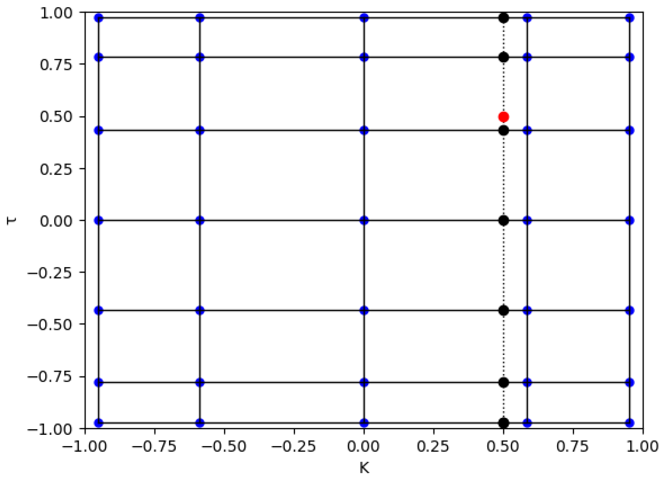Let us explain how it works; start with the two-dimensional case $(K,\tau ),$ with strike K and time to maturity $\tau ,$ and then proceed to the higher dimensions with $(K,\tau ,\gamma ,\beta ).$ Firstly construct a two-dimensional grid of Chebyshev nodes $C_2$ such that it has the following shape $N^{C_2}=(n_{strike},n_{\tau })$, where $n_{strike}\left(n_{\tau }\right)$ is the number of Chebyshev nodes selected for each parameter; any pair $\in C_2$ has the following form:

$$\{\widehat{x_k}=cos\left({\displaystyle \frac{(2k-1)\pi }{2n_{strike}}}\right),\widehat{x_t}=cos\left({\displaystyle \frac{(2t-1)\pi }{2n_{\tau }}}\right)\}$$

where strikes $k=1\dots n_{strike},$ and time to maturity $t=1\dots n_{\tau }.$ Next let $X_k$ be the set of $\widehat{x_k}$, and $X_t$ the set of $\widehat{x_t}.$ The grid is shown in Figure 1, where the Chebyshev node pairs are represented by those blue dots. In this plot, recall the one-dimensional case, so one can visualize this two-dimensional case as a stack of one-dimensional cases. Each horizontal (vertical) solid black line stacks vertically (horizontally) from this two-dimensional grid.

Suppose we wish to evaluate the function at a random point $(x_{k_i},x_{t_i})$, as follows:

$\mathrm{If}(x_{k_i},x_{t_i})\mathrm{is}\mathrm{the}\mathrm{point}\mathrm{on}\mathrm{the}\mathrm{grid}(\mathrm{black}\mathrm{line}\mathrm{connected}\mathrm{by}\mathrm{blue}\mathrm{dots}):$

$$\begin{array}{c}\hfill \begin{array}{cc}\hfill \mathrm{if}{x}_{t_i}& \in X_t,\mathrm{then}:\hfill \\ \hfill & f(x_{k_i},x_{t_i})\approx p(x_{k_i},x_{t_i})=p\left(x_{k_i}\right)=\sum _{j=0}^{n_{strike}-1}{a}_j{T}_j\left(x_{k_i}\right)\hfill \\ \hfill & \mathrm{where}{a}_j={\displaystyle \frac{2}{n_{strike}}}\sum _{k=1}^{n_{strike}}f\left(\widehat{x_k}\right)T_j\left(\widehat{x_k}\right),a_0={\displaystyle \frac{1}{n_{strike}}}\sum _{k=1}^{n_{strike}}f\left(\widehat{x_k}\right)\hfill \\ \hfill & \mathrm{This}\mathrm{means}\mathrm{we}\mathrm{view}\mathrm{each}\mathrm{horizontal}\mathrm{black}\mathrm{line}\mathrm{as}\mathrm{a}\mathrm{one}-\mathrm{dimensional}\mathrm{grid}\hfill \\ \hfill & \mathrm{Chebyshev}\mathrm{interpolation}.\mathrm{Note}\mathrm{that}\mathrm{j}\mathrm{has}\mathrm{a}\max \mathrm{value}\mathrm{of}{n}_{nodes}-1,\hfill \\ \hfill & \sin \mathrm{ce}\mathrm{n}+1\mathrm{nodes}\mathrm{will}\mathrm{be}\mathrm{choosen}\mathrm{for}\mathrm{a}\mathrm{n}\mathrm{degree}\mathrm{interpolation}.\hfill \\ \hfill \mathrm{if}{x}_{k_i}& \in X_k,\mathrm{then}:\hfill \\ \hfill & f(x_{k_i},x_{t_i})\approx p(x_{k_i},x_{t_i})=p\left(x_{t_i}\right)=\sum _{j=0}^{n_{\tau }-1}{a}_j{T}_j\left(x_{t_i}\right)\hfill \\ \hfill & \mathrm{where}{a}_j={\displaystyle \frac{2}{n_{\tau }}}\sum _{t=1}^{n_{\tau }}f\left(\widehat{x_t}\right)T_j\left(\widehat{x_t}\right),a_0={\displaystyle \frac{1}{n_{\tau }}}\sum _{t=1}^{n_{\tau }}f\left(\widehat{x_t}\right)\hfill \\ \hfill & \mathrm{This}\mathrm{means}\mathrm{we}\mathrm{view}\mathrm{each}\mathrm{vertical}\mathrm{black}\mathrm{line}\mathrm{as}\mathrm{a}\mathrm{one}-\mathrm{dimensional}\mathrm{grid}\hfill \\ \hfill & \mathrm{Chebyshev}\mathrm{interpolation}.\hfill \end{array}\end{array}$$

(9)

otherwise, $(x_{k_i},x_{t_i})$ is not on the grid, shown as the red dot in Figure 1:

$$\begin{array}{c}\hfill \begin{array}{cc}\hfill & \mathrm{In}\mathrm{the}\mathrm{following},\mathrm{the}\mathrm{function}\mathrm{values}\mathrm{at}\mathrm{each}\mathrm{black}\mathrm{dot}\mathrm{are}\mathrm{estimated}\hfill \\ \hfill & \mathrm{to}\mathrm{construct}\mathrm{a}\mathrm{vertical}\mathrm{one}\mathrm{dimension}\mathrm{interpolation}\mathrm{as}\mathrm{the}\hfill \\ \hfill & \mathrm{dashed}\mathrm{line}\mathrm{shown}\mathrm{in}\mathrm{the}\mathrm{Figure}:\hfill \\ \hfill & \forall \widehat{x_t}\in X_t,f_t(x_{k_i},\widehat{x_t})\approx p_t(x_{k_i},\widehat{x_t})=p_t\left(x_{k_i}\right)=\sum _{j=0}^{n_{strike}-1}{a}_j{T}_j\left(x_{k_i}\right)\hfill \\ \hfill & \mathrm{where}\mathrm{t}=1\dots n_{\tau },\mathrm{such}\mathrm{that}\mathrm{each}{p}_t\mathrm{represent}\mathrm{an}\mathrm{approximation}\hfill \\ \hfill & \mathrm{value}\mathrm{for}\mathrm{each}\mathrm{black}\mathrm{dot}\mathrm{at}{x}_{k_i}.\hfill \\ \hfill & \mathrm{Then},f(x_{k_i},x_{t_i})\approx p(x_{k_i},x_{t_i})=p\left(x_{t_i}\right)=\sum _{j=0}^{n_{\tau }-1}{a}_j{T}_j\left(x_{t_i}\right)\hfill \\ \hfill & \mathrm{where}{a}_j={\displaystyle \frac{2}{n_{\tau }}}\sum _{t=1}^{n_{\tau }}f\left(\widehat{x_t}\right)T_j\left(\widehat{x_t}\right)\approx {\displaystyle \frac{2}{n_{\tau }}}\sum _{t=1}^{n_{\tau }}{p}_t(x_{k_i},\widehat{x_t})T_j\left(\widehat{x_t}\right)\hfill \end{array}\end{array}$$

(10)

Next, let us consider the three-dimensional case ($K,\tau ,\gamma$), and the goal is to evaluate the function at a random point $(x_{k_i},x_{t_i},x_{{\gamma }_i}).$ Next, construct a three-dimensional grid of Chebyshev nodes $C_3$ as shown in Figure 2 such that it has the following shape $N^{C_3}=(n_{strike},n_{\tau },n_{\gamma }$), where $n_{strike},n_{\tau },n_{\gamma }$ is the number of Chebyshev nodes selected for each parameter. Every pair in $C_3,$ has the following form:

$$\{\widehat{x_k}=cos\left({\displaystyle \frac{(2k-1)\pi }{2n_{strike}}}\right),\widehat{x_t}=cos\left({\displaystyle \frac{(2t-1)\pi }{2n_{\tau }}}\right),\widehat{x_g}=cos\left({\displaystyle \frac{(2g-1)\pi }{2n_{\gamma }}}\right)\}$$

where k = 1…$n_{strike}$, t = 1…$n_{\tau }$, and g = 1…$n_{\gamma }.$ Let $X_k$ be the set of $\widehat{x_k}$, $X_t$ be set of $\widehat{x_t}$, and $X_g$ be set of $\widehat{x_g}$. One can visualize this three-dimensional grid as several two-dimensional grids stacked vertically, and then one can evaluate the function value for each red dot $x_{k_i},x_{t_i},\widehat{x_g}$ on those two-dimensional grids, thus creating a red line connecting those red dots (based on formula of (9) and (10)) to perform a one-dimensional Chebyshev interpolation; this is done similarly to the two-dimensional case (it evaluates the random point shown as the green dot in Figure 2.

Any random point $(x_{k_i},x_{t_i},x_{{\gamma }_i})$ which is not on the three-dimensional grid is shown as the green dot in Figure 1. The algorithm then works as follows:

$$\begin{array}{c}\hfill \begin{array}{cc}\hfill & \forall \widehat{x_g}\in X_g,f_t(x_{k_i},x_{t_i},\widehat{x_g})\approx p_g(x_{k_i},x_{t_i},\widehat{x_g})=p_g(x_{k_i},x_{t_i})\hfill \\ \hfill & \mathrm{result}\mathrm{given}\mathrm{by}\left(10\right).\hfill \\ \hfill & \mathrm{Here}\mathrm{g}=1\dots n_{\gamma },\mathrm{such}\mathrm{that}\mathrm{each}{p}_g\mathrm{represent}\mathrm{an}\mathrm{approximation}\hfill \\ \hfill & \mathrm{value}\mathrm{for}\mathrm{each}\mathrm{red}\mathrm{dot}\mathrm{at}{x}_{k_i}\mathrm{and}{x}_{t_i}\hfill \\ \hfill & \mathrm{Then},f(x_{k_i},x_{t_i},x_{g_i})\approx p(x_{k_i},x_{t_i},x_{g_i})=p\left(x_{g_i}\right)=\sum _{j=0}^{n_{\gamma }-1}{a}_j{T}_j\left(x_{g_i}\right)\hfill \\ \hfill & \mathrm{where}{a}_j={\displaystyle \frac{2}{n_{\gamma }}}\sum _{g=1}^{n_{\gamma }}f\left(\widehat{x_g}\right)T_j\left(\widehat{x_g}\right)\approx {\displaystyle \frac{2}{n_{\gamma }}}\sum _{g=1}^{n_{\gamma }}{p}_g(x_{k_i},x_{t_i},\widehat{x_g})T_j\left(\widehat{x_g}\right)\hfill \end{array}\end{array}$$

(11)

For the four-dimensional case, as in the three-dimensional case, one can visualize the four-dimensional grid as several three-dimensional grid stacked together; the method is now clear and as such the details are omitted.

4.3. Calibration Result and Error Analysis

The calibration uses the same criteria and synthetic data of Section 3. Consider the finite liquidity price of an European Call Spread with four input variables—$\gamma ,\beta ,K,\tau$. We first set up a four-dimensional Chebyshev grid and determine its shape (see

Table 1. Shape of 4-dimensional Chebyshev meshgrid.

Parameter	Boundary	n Nodes
$\gamma$	[0.049, 1.01]	11
$\beta$	[9.99, 100.01]	6
K	[0, 10.1]	11
$\tau$	[0.04999, 1.0001]	11

).

Next, we employ Monte Carlo simulation to compute the spread option prices corresponding to the Chebyshev nodes, as summarized in

Table 2. Simulated training data for Chebyshev interpolation.

$\mathit{\gamma }$	$\mathit{\beta }$	Strike	$\mathit{\tau }$	Monte Carlo Price
1.01	100.01	10.1	1.0001	2.499332
0.986483	100.01	10.1	1.0001	2.505044
0.918233	100.01	10.1	1.0001	2.499176
0.811931	100.01	10.1	1.0001	2.485744
…	…	…	…	…
0.072517	9.99	0	0.04999	9.935221
0.04900	9.99	0	0.04999	9.935031

, resulting in a dataset of 7986 price points. The parameter boundaries chosen for this simulation are intended solely for illustrative purposes. In practical applications, these ranges should be adjusted dynamically to reflect prevailing market conditions. For instance, the time to maturity $\tau$ may extend beyond one year, and $\gamma ,\beta$ may assume larger values in environments characterized by heightened illiquidity.

The number of Chebyshev nodes can also be adjusted according to the desired interpolation accuracy. Increasing the number of nodes per dimension enhances the precision of the interpolated pricing function. However, this improvement comes at the cost of a significantly higher computational burden, as the total number of required training points grows exponentially with dimensionality. This trade-off between accuracy and computational cost is examined in greater detail (see Section 4.3.1).

The following calibration result in

Table 3. Calibration result and comparison.

Method	$\mathit{\gamma }$	$\mathit{\beta }$	SSE
Chebyshev	0.56992281	67.85215697	17.5903918
Non linear regression	0.61998133	73.54941529	59.9923119

is obtained by applying the method of Section 4.2.

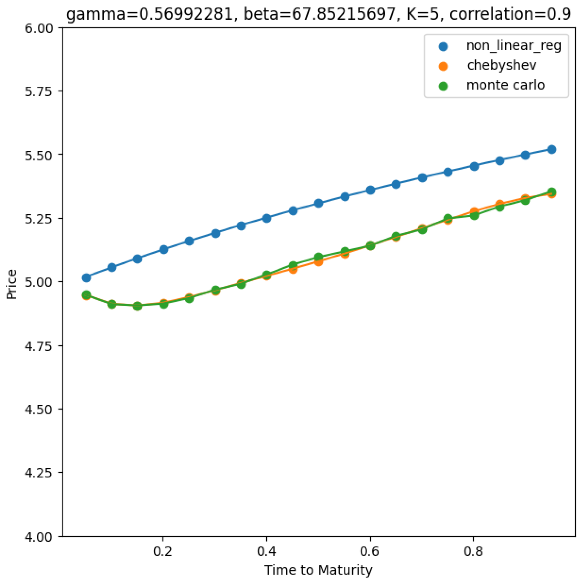
Both methods yield similar results for calibrated parameters, with Chebyshev interpolation giving a lower SSE (SSE between Chebyshev estimated price and synthetic price), thus providing a more accurate calibration result to exogeneous data. A comparison of non-linear regression and Chebyshev interpolation results against the Monte Carlo price (with same model parameter) is displayed in Figure 3, and this is further discussed in Section 4.3.2.

4.3.1. Trade-Off Between Accuracy and Training Cost for Chebyshev Interpolation

As illustrated in the previous section, Chebyshev interpolation requires evaluating the option price at each Chebyshev node. In our case, this results in 7986 computations using Antithetic Monte Carlo simulation, with each simulation involving 30,000 correlated stock price paths. The total computational time for this process is approximately six hours. We selected six nodes for the parameter $\beta ,$ as it is not a primary driver of the pricing function. As seen in Equation (1), $\beta$ primarily governs the rate at which the intensity function $\lambda \left(t\right)$ approaches its maximum value $\gamma$ over the time horizon. This observation is supported by numerical evidence from Pirvu and Zhang (2024), where similar conclusions were drawn. Therefore, a lower number of interpolation nodes for $\beta$ is sufficient, and we will examine the impact of this choice in subsequent analysis.

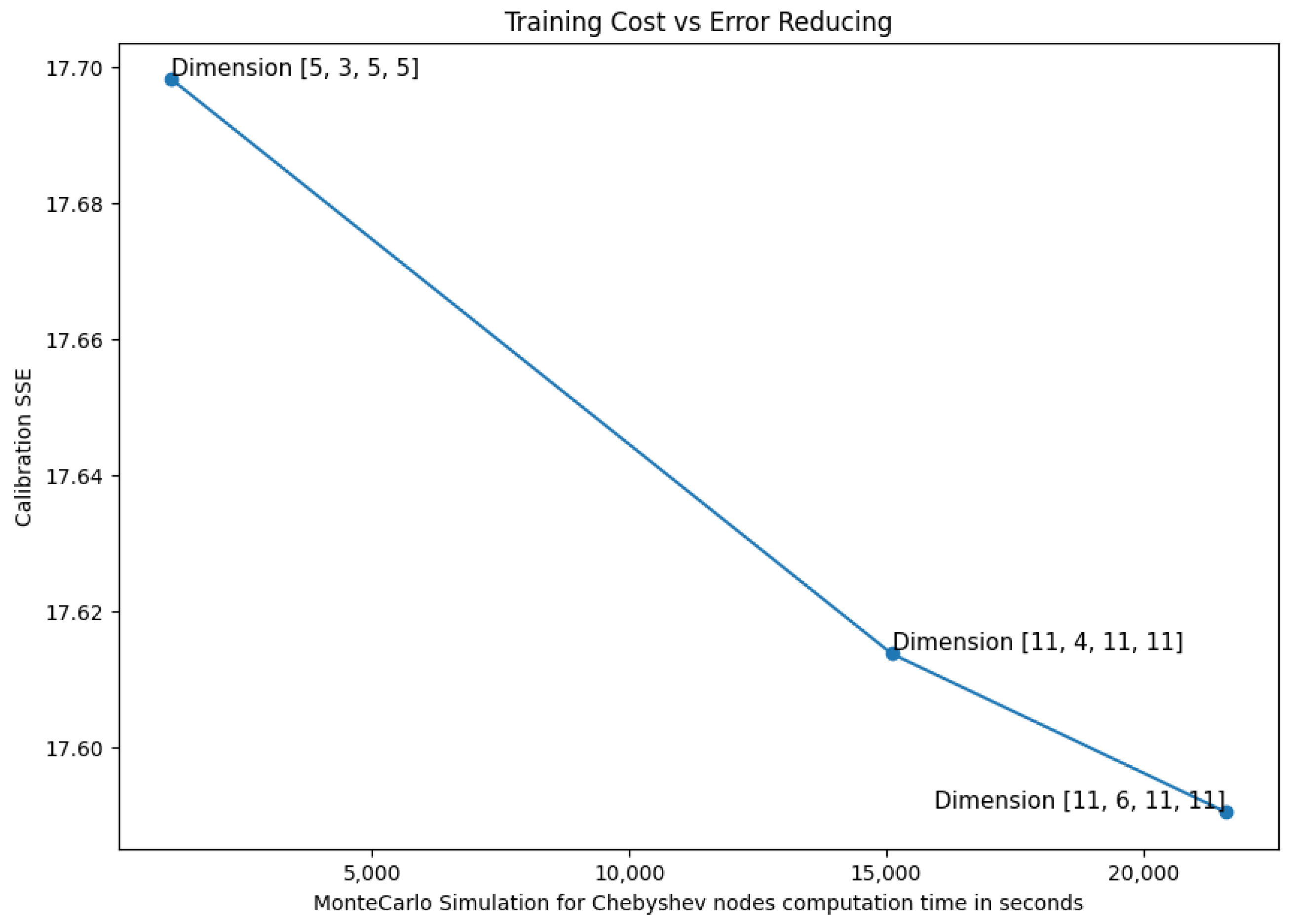
We constructed three four-dimensional Chebyshev grids with varying configurations of interpolation nodes across the parameters [$\gamma$, $\beta$, Strike, $\tau$], as detailed in

Table 4. Shape of Chebyshev grid for comparison.

	Shape	Training Time (s)	$\mathit{\gamma }$	$\mathit{\beta }$	SSE
1	[5, 3, 5, 5]	1100	0.51020	70.64183	17.69825
2	[11, 4, 11, 11]	15100	0.55945	71.54141	17.61378
3	[11, 6, 11, 11]	21600	0.56993	67.85216	17.59039

to examine the trade-off between interpolation accuracy and training cost in the Chebyshev framework. The corresponding computational times for generating each grid were also recorded. Subsequently, we performed parameter calibration using each of the three grids, and the resulting outcomes are presented in Table 4. Let us point out a marginally lower SSE for the grid with a higher number of Chebyshev nodes. Moreover, each grid results in similar calibrated parameters. However, the improvement in accuracy is relatively limited, while the associated computational time increases substantially. This diminishing return is illustrated in Figure 4.

4.3.2. Calibration Error Analysis

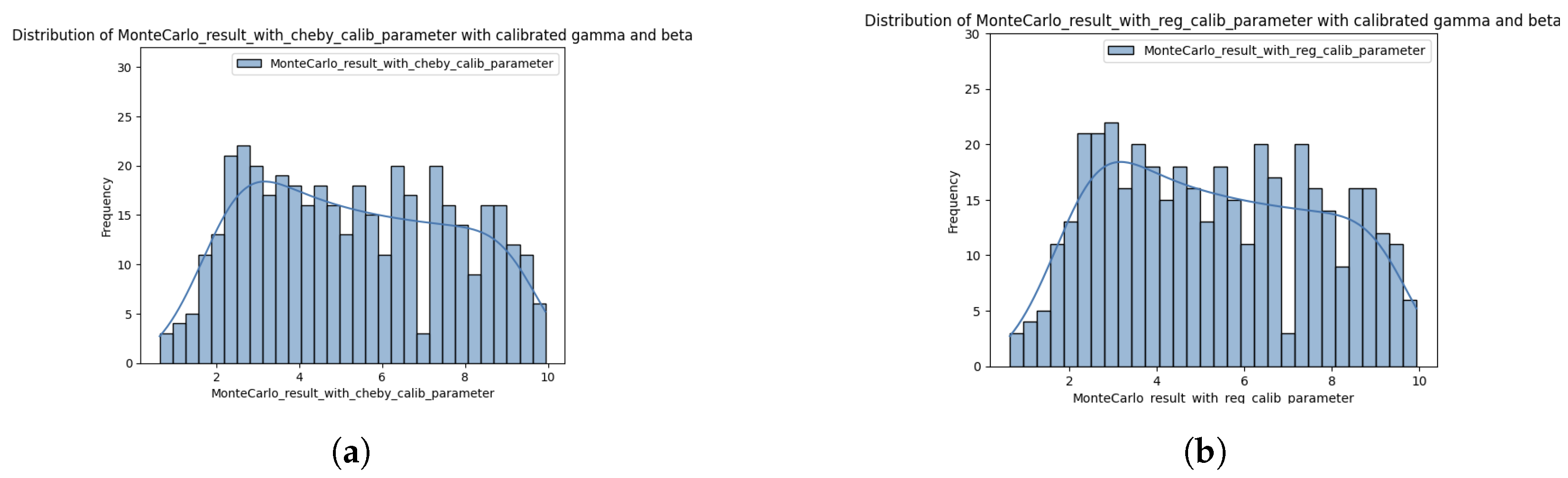
In this section, we conduct a more detailed examination and visualization of the performance of the two estimation methods in replicating the prices obtained by Monte Carlo simulation. To further evaluate the validity of our calibration approach, we apply the two-sample t-test, and the Kolmogorov-Smirnov (KS) test to statistically compare the distributions of the estimated/interpolated prices and the Monte Carlo simulated prices.

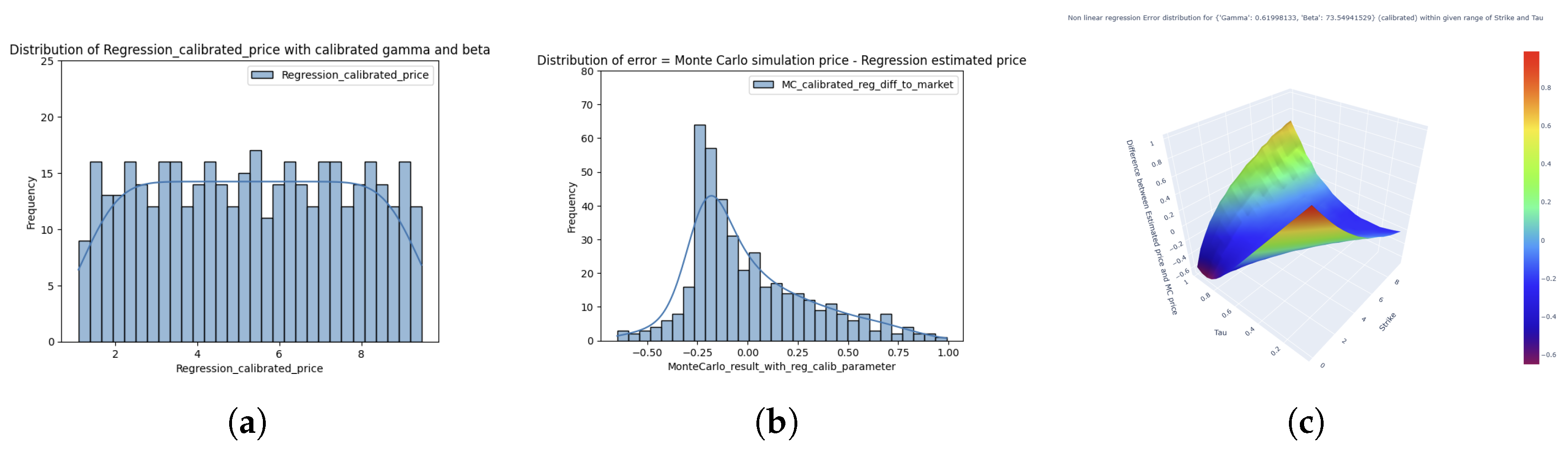
Let us begin by presenting the distribution of Monte Carlo simulated prices generated by the calibrated parameters obtained by the two calibration methods (see Figure 5). Figure 6 presents the distribution of the prices produced by Chebyshev interpolation along with their deviations from the Monte Carlo simulated prices. In parallel, Figure 7 illustrates the regression-based estimates and the corresponding error distribution. The Chebyshev interpolation method exhibits a notably narrower error distribution with reduced tail behavior, and more uniform spread of error across the pricing surface. In contrast, the regression-based errors are more dispersed in the right tail, indicating higher localized discrepancies, especially in the extreme ends of the parameter domain. Furthermore, the distribution of estimated values from both methods highlights the superior accuracy of Chebyshev interpolation, which more closely replicates the Monte Carlo simulated prices when compared to the regression-based approach.

The results of the two statistical tests are shown in

Table 5. Test statistics and p value.

Method	Tstat	Tpvalue	KSstat	KSpvalue	Significance
Chebyshev	0.009803	0.992181	0.007143	1.0	True
Non linear regression	0.004112	0.99672	0.040476	0.882137	True

, and the corresponding cumulative distribution functions (CDF) are depicted in Figure 8. These results support the conclusions drawn in the preceding analysis. While the two methods yield comparable t-test statistics, the Chebyshev interpolation demonstrates superior performance in the Kolmogorov-Smirnov (KS) test. Specifically, the CDF of prices estimated via Chebyshev interpolation closely aligns with that of the Monte Carlo simulation, indicating a more accurate overall distributional match.

4.4. Practical Implications

As a practical implication we report on the liquidity value adjustment (LVA) of our model. The impact of calibrated parameters on the price of spread option across various combinations of strike price and time to maturity ($\tau$) is explored; the initial stock values are $S_1\left(0\right)=110,$ and $S_2\left(0\right)=100.$ The results reveal that the liquidity adjustment becomes more pronounced for out-of-the-money options than in the money option. This effect is explained by the additional drift term introduced in the stochastic differential equation governing $S_1,$ which increases the likelihood of the option ending up in the money at maturity. Consequently, the option’s fair price rises to compensate for the elevated hedging costs faced by the writer under illiquid conditions (see

Table 6. Kirk approximation of perfect liquidity price with calibrated parameters.

	τ	0.2	0.4	0.6	0.8	1.0
Strike
2 (ITM)		7.7738	7.6405	7.58	7.5545	7.5456
15 (OTM)		0.0524	0.2147	0.3936	0.5652	0.725

,

Table 7. Monte Carlo simulation of finite liquidity price with calibrated parameter.

	τ	0.2	0.4	0.6	0.8	1.0
Strike
2 (ITM)		7.7754	7.6597	7.6129	7.6055	7.5999
15 (OTM)		0.0629	0.2516	0.4398	0.6168	0.7866

,

Table 8. LVA as relative difference.

	τ	0.2	0.4	0.6	0.8	1.0
Strike
2 (ITM)		0.02%	0.25%	0.43%	0.68%	0.72%
15 (OTM)		19.97%	17.18%	11.73%	9.14%	8.49%

and

Table 9. LVA as real difference.

	τ	0.2	0.4	0.6	0.8	1.0
Strike
2 (ITM)		0.0016	0.0192	0.0329	0.051	0.0543
15 (OTM)		0.0105	0.0369	0.0462	0.0517	0.0616

).

5. Conclusions

Our paper provides a novel calibration procedure for pricing spread options with a liquidity risk model. This is achieved by means of Chebyshev interpolation, which fits the prices obtained by Pirvu and Zhang (2024). The multi-dimensional Chebyshev interpolation is reduced to a one-dimensional Chebyshev interpolation by a dimensionality reduction technique. The calibration obtained by this paper performs better than the one of Pirvu and Zhang (2025), as shown by numerical experiments.