Article

Modeling Age-to-Age Development Factors in Auto Insurance Through Principal Component Analysis and Temporal Clustering

Global Management Studies, Ted Rogers School of Management, Toronto Metropolitan University, Toronto, ON M5B 2K3, Canada
*
Author to whom correspondence should be addressed.
Risks 2025, 13(6), 100; https://doi.org/10.3390/risks13060100
Submission received: 15 April 2025 / Revised: 14 May 2025 / Accepted: 16 May 2025 / Published: 22 May 2025

Abstract

:
The estimation of age-to-age development factors is fundamental to loss reserving, with direct implications for risk management and regulatory compliance in the auto insurance sector. The precise and robust estimation of these factors underpins the credibility of case reserves and the effective management of future claim liabilities. This study investigates the underlying structure and sources of variability in development factor estimates by applying multivariate statistical techniques to the analysis of development triangles. Departing from conventional univariate summaries (e.g., mean or median), we introduce a comprehensive framework that incorporates temporal clustering of development factors and addresses associated modeling complexities, including high dimensionality and temporal dependency. The proposed methodology enhances interpretability and captures latent structures in the data, thereby improving the reliability of reserve estimates. Our findings contribute to the advancement of reserving practices by offering a more nuanced understanding of development factor behavior under uncertainty.

1. Introduction

Age-to-age loss development factors (LDFs) are fundamental tools in property and casualty insurance, enabling the projection of future claim amounts. These projections are derived from observed claims organized in loss development triangles, with the primary goal of estimating future development. When applied to claim counts, these factors are referred to as count development factors. The accurate estimation of development factors (DFs) is crucial for effective risk assessment and the management of future financial liabilities. As highlighted in Berquist and Sherman (1977), DFs are integral to forecasting ultimate losses or claim counts. Furthermore, they offer insights into claim payment patterns (Pittarello et al. 2022; Shi and Hartman 2016), supporting financial planning in auto insurance.
Despite notable advancements in DF estimation, much of the literature remains anchored in traditional methods, each with distinct advantages and limitations (Berquist and Sherman 1977; D’Arcy 1987; Okyere Dwebeng 2016). Among these, the Chain Ladder method (Verrall 2000) is widely used for its simplicity, estimating DFs by tracking the progression of claims over time. However, it often performs poorly under volatile development conditions. The Bornhuetter–Ferguson method (Schmidt and Zocher 2007), a hybrid of the Chain Ladder and Expected Loss Ratio approaches, combines historical data with prior estimates of ultimate losses (Sakthivel 2016). While more stable, it is sensitive to prior assumptions and introduces additional uncertainty through its reliance on paid loss information. The Cape Cod method, an extension of Bornhuetter–Ferguson, can yield more accurate estimates but requires extensive internal and external data and greater computational resources (Radtke 2016). The Mack model (Kloek 1998), a stochastic extension of the Chain Ladder, assumes development factors follow specific distributions (e.g., log-normal), thereby allowing for stochastic reserving via Generalized Linear Models. This enhances estimation flexibility and enables the quantification of reserve uncertainty.
Our research shifts the focus from traditional age-to-age DF estimation to an in-depth analysis of the variability and structural patterns of DFs. Recent studies have explored refined estimation techniques for DFs to improve reserving accuracy (Han and Gau 2008; Jeong and Dey 2020; Jeong et al. 2021; Korn 2015; Verdier and Klinger 2005), reflecting a broader commitment to predictive analytics and financial stability in the insurance sector. However, DF estimates are subject to uncertainty stemming from model assumptions, small sample sizes, evolving claim patterns, and data quality issues (Feng and Robbin 2022; Mack 1995; Nugraha and Qoyyimi 2022; Raço et al. 2022). This inherent variability challenges the reliability of case reserve forecasts. Stochastic reserving models have thus gained traction as alternatives to deterministic approaches, incorporating statistical tools such as regression and time-series analysis, often complemented by actuarial judgment (Al-Mudafer et al. 2022; England and Verrall 2002; Sriram and Shi 2021; Taylor 2012).
To address these challenges, we propose further analysis of Development Rectangles (DRs), which aggregate age-to-age DFs across accident half-years. DRs help identify longitudinal and cross-sectional trends in loss development, which are often obscured in raw triangle data. Detecting such trends can improve reserving accuracy and inform regulatory pricing strategies (Frees et al. 2014). Moreover, DRs facilitate the identification of outliers—extreme values that, if uncorrected, may skew DF estimates and misrepresent future liabilities (Zhao et al. 2021). To mitigate this, de-noising techniques tailored to DRs have been proposed (Barlak et al. 2022; Neuhaus 2023), emphasizing the need for context-specific methods.
In this study, we analyze DRs derived from various regulatory datasets, focusing on incurred loss, paid loss, claim counts, and paid counts. Using the Mack model (Mack 1999), we construct DRs across different reporting periods and apply Principal Component Analysis (PCA) to uncover latent patterns of variation. Rather than developing new reserving methodologies, our contribution lies in promoting the use of multivariate statistical techniques for pattern discovery and uncertainty quantification in DFs. This approach enhances our understanding of variation across accident half-years and improves risk assessment under regulatory frameworks.
A key innovation in this study is the introduction of a time-constrained, weighted K-Means algorithm, which extends the classical K-Means by restricting cluster formation to temporally adjacent accident half-years. This constraint increases the interpretability and relevance of clustering results in the context of loss reserving, enabling the detection of evolving structural changes in development factors. Moreover, the exploration of DF patterns using industry-level data adds a unique and novel dimension to this study.
Ultimately, our approach advances the use of predictive analytics in the actuarial domain, with implications for pricing strategy and reserve adequacy. The remainder of the paper is structured as follows: Section 2 describes the data and methodology. Section 3 presents and interprets empirical findings based on regulatory datasets. Section 5 concludes the paper and outlines directions for future research.

2. Materials and Methods

2.1. Data

The dataset analyzed in this study comprises incurred loss development, incurred claim count development, paid claim count development, and paid loss development for accident half-years spanning from 2003-1 to 2017-2 as reported at six-month intervals through 31 December 2017. For subsequent accident half-years from 2004-1 to 2018-2, development is reported as of year-end 2018. This structure applies across valuation years from 2017 through 2022, which form the basis of our analysis. Both incurred and paid loss amounts include associated settlement expenses, thereby reflecting the full cost of claim resolution. To enhance the homogeneity of development patterns, development triangles are constructed separately for major coverage types—medical, bodily injury (BI), and collision. These triangles are generated using a custom-built program in R software package, and the corresponding development rectangles are derived using the Mack Chain Ladder model, a widely adopted method in actuarial practice for case reserving.
For illustration purposes, Table 1 presents an example of BI incurred loss development factor rectangles for development ages up to 72 months. This table is based on data from the 2022 reporting year. As a result, the age-to-age development factor for the first 6 months of accident half-year 2022-02 is an estimated value, while the corresponding factor for 2022-01 is a calculated value derived from observed incurred losses. In this context, the values in the last row of Table 1 are entirely estimated. Estimation begins from the second-last row and proceeds backward, except for the portion on the left side of the table, where the accident half-year plus development period does not exceed the reporting year. For example, the accident half-year 2021-02 plus an 18-month development period extends to the end of the 2022 calendar year, the reporting period. This means that the values 7.513 and 2.086 in that row are based on observed data, while the remaining values in the same row are estimates.
In this study, the primary focus is to analyze these projected development rectangles using multivariate statistical techniques, with the aim of better understanding the variability inherent in age-to-age development factors. As such, we do not delve into the full forecasting process used to construct the development rectangles but rather emphasize the investigation of variability patterns in the obtained rectangles. Additionally, we propose a Generalized Linear Model (GLM)-based approach to estimate the mean development factors at each development age. This framework allows us to explain variations in DFs by incorporating relevant covariates, thereby enhancing interpretability and predictive accuracy. We assume that input data are available in the form of a development triangle. Additionally, we assume that a forecasting method is in place and ready to be applied for predicting the unobserved values in the development rectangle.

2.2. Estimating Age-to-Age Development Factors via Principal Component Analysis

Principal Component Analysis (PCA) is a multivariate statistical technique widely used to explore complex patterns and dependencies in high-dimensional datasets. It achieves dimensionality reduction by identifying orthogonal directions, principal components, which capture the maximum variance in the data. By reconstructing the original data using only a subset of these components, PCA effectively filters out noise, leading to a de-noising effect. In the context of DRs, we treat each age-to-age DF as a distinct random variable, each with its own underlying expected value representing the true DF. Observations across different accident half years are interpreted as replicates of these random variables. Given the high dimensionality and complexity of DRs—each encoding a wide array of age-to-age development patterns—PCA provides a powerful framework for uncovering underlying structures and reducing dimensionality while preserving the majority of the variation.
By isolating the most influential DFs that contribute significantly to the variation in loss development, PCA enhances the interpretability, stability, and precision of models used for LDF estimation and future claims forecasting. Conceptually, the DR is viewed as comprising both signal and noise components. PCA enables the separation of these components by approximating the original data structure using only the leading principal components. Furthermore, PCA facilitates the quantification of uncertainty associated with DF estimates through the analysis of principal component scores. The integration of PCA-derived insights into the modeling process can significantly improve the robustness and accuracy of loss reserving methods, supporting insurers in risk management and assisting regulators in making data-informed pricing and policy decisions.
PCA can be implemented using two standard approaches: eigenvalue decomposition of the covariance matrix and singular value decomposition (SVD) of the data matrix. For completeness and clarity, we briefly outline the eigenvalue decomposition method for performing PCA in the following section.

2.3. Eigenvalue Decomposition of DR

Given a DR with n accident half years and p development periods—each considered a random variable—we denote the observed data as an n × p matrix L. The first step in PCA is to standardize the data by subtracting the mean and dividing by the standard deviation of each variable. This results in a standardized matrix Z. The sample mean of the p-dimensional random vector provides an empirical estimate of the DF at each development age, while the sample standard deviation captures the uncertainty contributed by each accident year’s development data and by the method used to project unobserved points in the DR. The sample covariance matrix of Z, denoted by C, is a p × p matrix given by
C = 1 n 1 Z Z .
This covariance matrix reflects the uncertainty arising from accident half year variation, the correlation among development ages, and the variability introduced by the projection methodology. The concentration of variations across development ages helps assess the temporal robustness of DF patterns. To further examine this structure, we perform an eigenvalue decomposition of the covariance matrix C, resulting in eigenvectors and eigenvalues. The eigenvectors represent the principal components of the DFs, while the eigenvalues quantify the amount of variance captured by each component. These eigenvectors are ordered by decreasing eigenvalues.
We select the top k principal components based on the desired level of variance explained, denoted by q. For instance, if q = 95 % , we choose the smallest k such that the sum of the first k eigenvalues is at least 95% of the total variance. In this work, we investigate how many components are necessary to capture the dominant fluctuations in age-to-age development factors across accident years. Let V ( k ) R p × k be the matrix containing the first k eigenvectors. The matrix of principal component scores, T ( k ) R n × k , is computed as
T ( k ) = Z V ( k ) .
Each row of T ( k ) corresponds to the projection of an accident year onto the reduced k-dimensional space defined by the principal components. We then approximate the original data matrix L using the selected k components, yielding
L ( k ) = T ( k ) V ( k ) + L ¯ ,
where L ¯ is the row vector of column means of the original DR data, repeated across all rows. We denote the approximations using the first and first two components as L ( 1 ) and L ( 2 ) , respectively. The first and second principal component vectors are V 1 ( k ) and V 2 ( k ) , and their associated score vectors are T 1 ( k ) and T 2 ( k ) .
This low-rank approximation helps reduce the influence of noise and potential outliers in the DFs. By focusing on the major components, the reconstruction preserves the underlying development patterns while filtering out irregular fluctuations, thereby enhancing the interpretability and robustness of the loss development analysis.

2.4. K-Means Clustering of Principal Component Scores with Contiguity Constraints in Time

Principal component scores serve as key features for exploring the characteristics of DFs within a reduced, low-dimensional feature space. These scores capture both the magnitude of each principal component and the variability of features across accident years. When analyzing DFs over time, it is natural to consider temporal contiguity, i.e., the idea that neighboring accident half years are likely to exhibit similar development patterns due to shared economic conditions, inflationary trends, and safety-related advancements that influence incurred losses or claim counts. This notion parallels spatial clustering in auto insurance pricing, where geographical proximity is used to ensure spatial continuity in risk segmentation. Similarly, temporal contiguity should be preserved when clustering accident half years based on their development profiles.
To incorporate this insight, we propose a novel clustering algorithm that assigns a weight to each feature prior to applying the K-Means clustering method. The optimal weight value is selected by minimizing a metric that quantifies cluster contiguity—specifically, the total number of temporally disjoint observations within clusters. The primary objective of this algorithm is to balance clustering performance with the requirement that accident half years grouped within a cluster exhibit temporal continuity. This emphasis on contiguity is grounded in the assumption that adjacent accident years should demonstrate shared characteristics in their DF trajectories. The algorithmic procedure is outlined in Algorithm 1, where two key innovations are introduced to the traditional K-Means approach:
Algorithm 1 Procedure for K-Means clustering of principal component scores with contiguity constraints in time.
1:
Perform the PCA on the covariance matrix of the data, and compute the variance ( λ i ) for the ith PC. Select the smallest number of components k such that
i = 1 k λ i i = 1 N 1 λ i > q ,
where 0 < q < 1 , and N is the total number of Accident Half-Year. By default, q = 0.95 .
2:
Construct dataset including two components: PC scores for the first kth PCs, and an additional column representing Accident Half-Year, ranging from 1 to N. Scale this data and denote it by D, where D can be written as ( P S 1 , , P S k , t ) .
3:
For each pre-specified scalar value of w,
a: Create new dataset D w , where D w = ( P S 1 w , . . . , P S k w , t ( 1 w k ) ) n k .
b: Apply K-Means clustering methods on D w , and extract the cluster number that each observation belongs to. Reorganize the cluster numbers in ascending order, denoted by c w , where c w = ( c 1 w , . . . , c n w ) and n is the number of observations.
c: Use C T w to quantify the contiguity of the clusters,
C T w = #   of   ( c ( i + 1 ) w c i w ) < 0 n
for i = 1 , , n 1 .
4:
Minimize C T w with respect to w, then denote the corresponding membership of accident year as C a r g m i n w = ( c 1 , . . . , c n ) .
5:
Make the final adjustment for the membership assignment. Let M = ( m 1 , , m n ) represent the optimal membership of the accident year.
a:
m 1 c 1
b:
For i = 2 , , n 1 ,
c:
if  m i 1 = c i + 1  then  m i m i 1
d:
else  m i c i
  • A weight is incorporated into the objective function to control the influence of each feature during clustering.
  • Post-clustering adjustments are made to ensure that clusters maintain full temporal contiguity, and no cluster consists of a single, isolated accident half year.
These enhancements enable the clustering results to better reflect underlying temporal structures in the DR. The resulting clusters are subsequently used in downstream modeling, where age-to-age development factors are estimated at the cluster level. This approach generalizes the traditional method of estimating a single DF for each development age by incorporating group-level effects that account for shared characteristics among similar accident years.

2.5. Modeling Development Factors by Generalized Linear Models

In addition to using Principal Component Analysis to decompose the development rectangle and approximate the development pattern using a subset of principal components, we propose applying a Generalized Linear Model (GLM) to directly model the development factors within the DR. The GLM-based approach offers several advantages, including improved interpretability of loss or count development patterns and enhanced uncertainty quantification. By fitting a GLM to the DR data, one can obtain estimates of the age-to-age DFs along with their associated standard errors. These standard errors provide a direct measure of the uncertainty associated with the DF estimates. Moreover, the estimated residual standard deviation from the GLM model can be used to assess the overall reliability of the model and the stability of the DF estimates. This GLM-based approach contrasts with traditional methods, which typically rely on summary statistics—such as the sample mean or median across all accident years—to estimate each age-to-age DF. By leveraging regression modeling, our approach introduces flexibility to incorporate covariates that explain variation in DFs across time and groups.
In this section, we briefly describe the application of our GLM-based modeling for estimating age-to-age DFs. Let Y i , j represent the incurred losses (or counts) for the jth accident half year at the ith development period. The corresponding age-to-age development factor, denoted by d i j , is defined as the ratio of the ( i + 1 ) th to the ith period losses (or counts):
d i j = Y i + 1 , j Y i , j .
The response variable d i j is assumed to follow a distribution from the exponential family, characterized by the general form
f ( d θ , ϕ ) = exp d θ b ( θ ) a ( ϕ ) + c ( d , ϕ ) ,
where θ is the canonical parameter, ϕ is the dispersion parameter, and the functions a ( · ) , b ( · ) , and c ( · ) depend on the specific distribution family. The variance of d is given by
Var ( d ) = ϕ V ( μ ) ,
where V ( μ ) is the variance function that describes how the variance changes with the mean μ . For example, in a normal distribution, V ( μ ) = 1 , while in a Poisson distribution, V ( μ ) = μ .
Given that DFs are closely associated with the development period in which they are observed, we include ‘Period’ as a key covariate in our model. Additionally, to investigate whether clusters of accident years affect DF patterns, we introduce a dummy variable ‘Group’, with the earliest accident year group serving as the reference category. The predictor associated with GLM can thus be expressed as
g ( E ( d i j ) ) = β 0 + β 1 · Group i , j + β 2 · Period j ,
where g ( · ) is a link function used to linked mean response E ( d i j ) to the linear combination of covariates. Given that both Group and Period are categorical covariates, the estimated effects for each level represent the mean difference from the respective base level. The model is applied separately to data from each reporting year (e.g., 2020, 2021, and 2022) to capture time heterogeneity in the estimates. Parameter estimates in the GLM are obtained via iteratively reweighted least squares (IRWLS). For implementation, we use the glm function in R. When the response follows a normal distribution, the estimated DF for the ith development period can be calculated as β ^ 0 + β ^ i 2 , where the estimate also depends on the cluster to which the accident year belongs, through the coefficient β ^ 1 .

2.6. Implications of Proposed Methods

Traditional risk management in auto insurance has long relied on understanding the development of future liabilities through the projection of unobserved losses in loss development triangles or claim counts in count development triangles. A more detailed exploration of age-to-age development factors (DFs) in the reserving process offers significant potential to enhance both risk management and financial forecasting.
This study introduces a novel multivariate analysis of forecasted development factors, structured in rectangular form rather than conventional triangular models. This shift enables a better understanding of DF behavior, moving beyond summary statistics to examine patterns, variability, and dependencies. Such deeper insights not only refine the accuracy of case reserve estimates but also illuminate the inherent uncertainty and variability surrounding DF predictions. These improvements are critical for insurers aiming to make informed reserving decisions, optimize capital allocation, and more effectively manage portfolio risk. In doing so, this work contributes to more resilient and financially sound insurance operations.
Conventional approaches typically assume the independence of DFs across accident years—a simplification that fails to capture the evolving nature of insurance systems. In reality, development factors are influenced by a range of time-dependent variables, including improvements in vehicle safety technology, shifts in medical treatment standards, and changes in infrastructure or regional transportation systems. To account for these dynamics, our study advocates for the temporal clustering of development factors. By organizing DFs according to their position in time, rather than treating them as interchangeable across years, we uncover meaningful patterns that reflect systemic change. This temporal perspective allows for more accurate modeling of development behavior and ultimately leads to better-informed forecasting.
Our research highlights the practical advantages of this approach in modern auto insurance, offering a more adaptive framework that aligns with the complex, evolving realities of claims development. Temporal clustering not only strengthens predictive accuracy but also supports more flexible and responsive risk management strategies, an essential advancement for navigating today’s dynamic insurance landscape.

3. Results

3.1. Results on Principal Component Analysis and Weighted K-Means of Development Factors

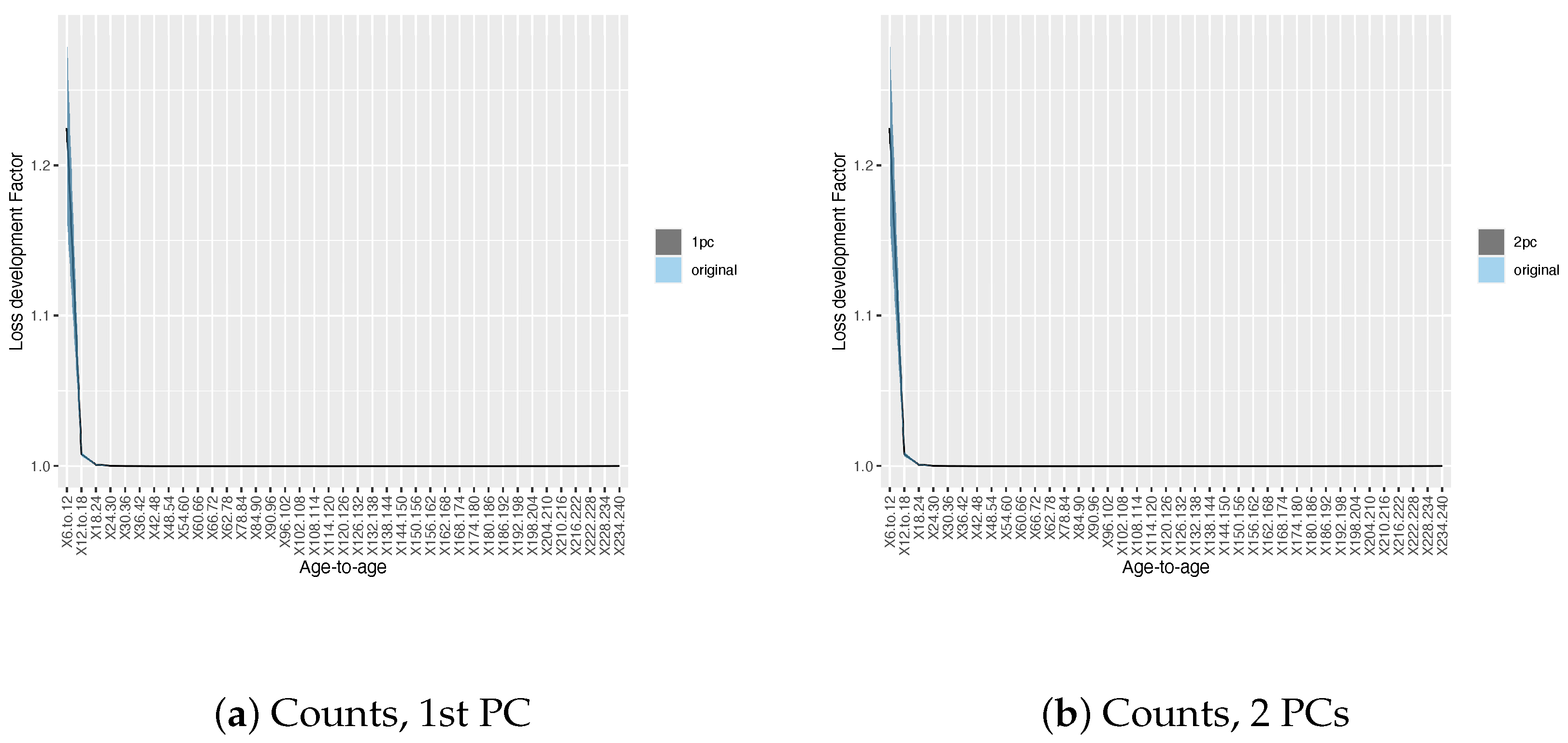
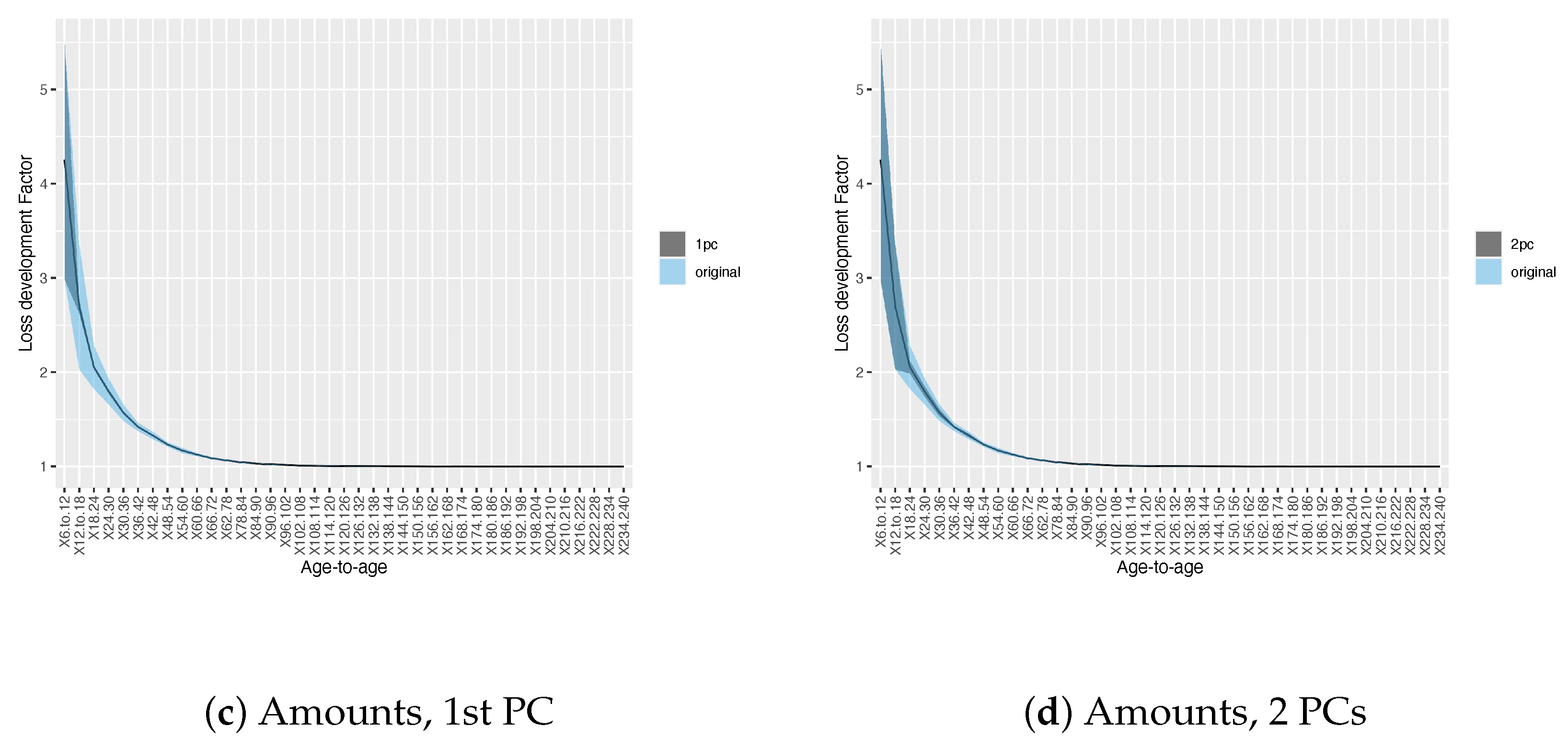
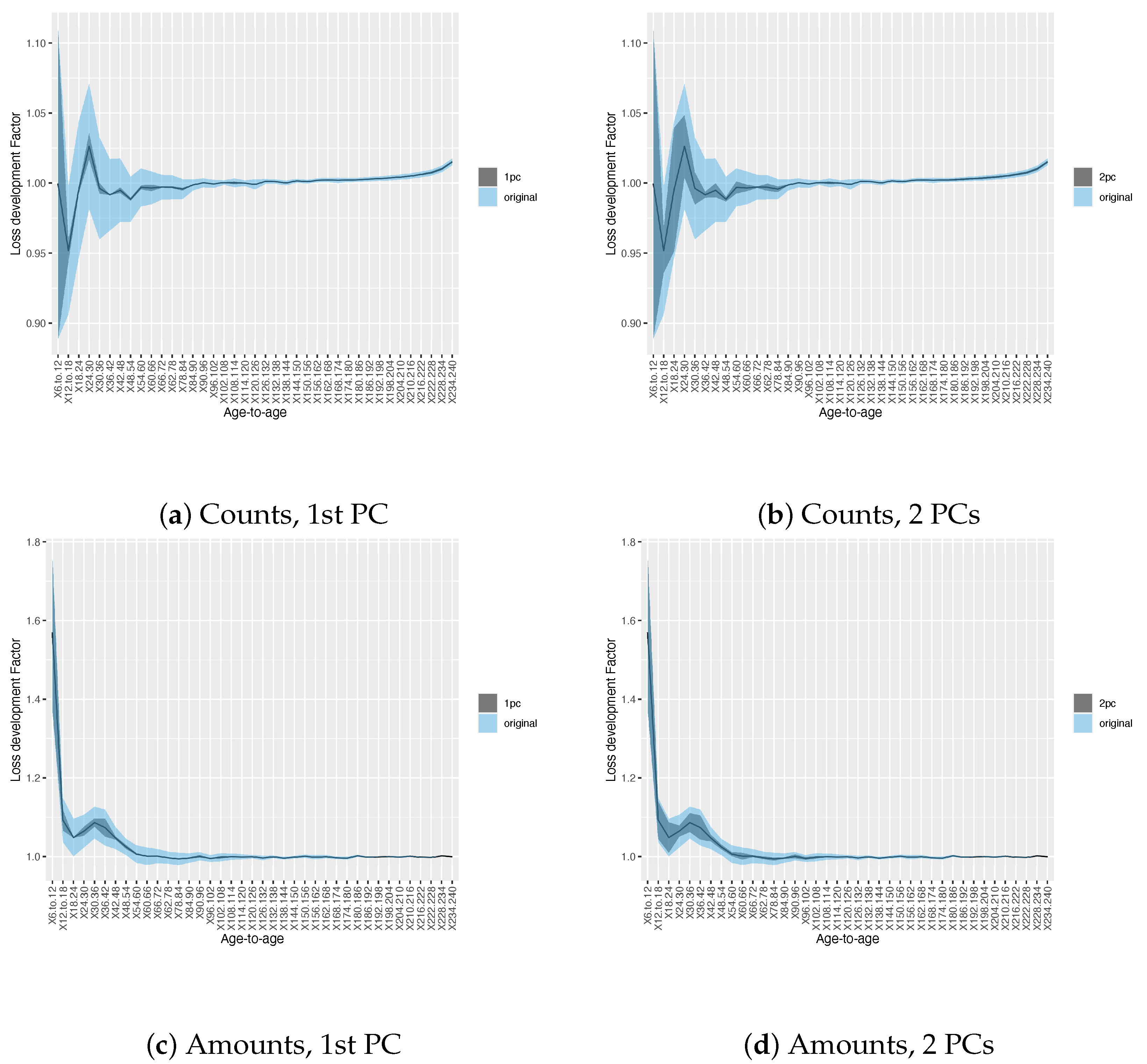
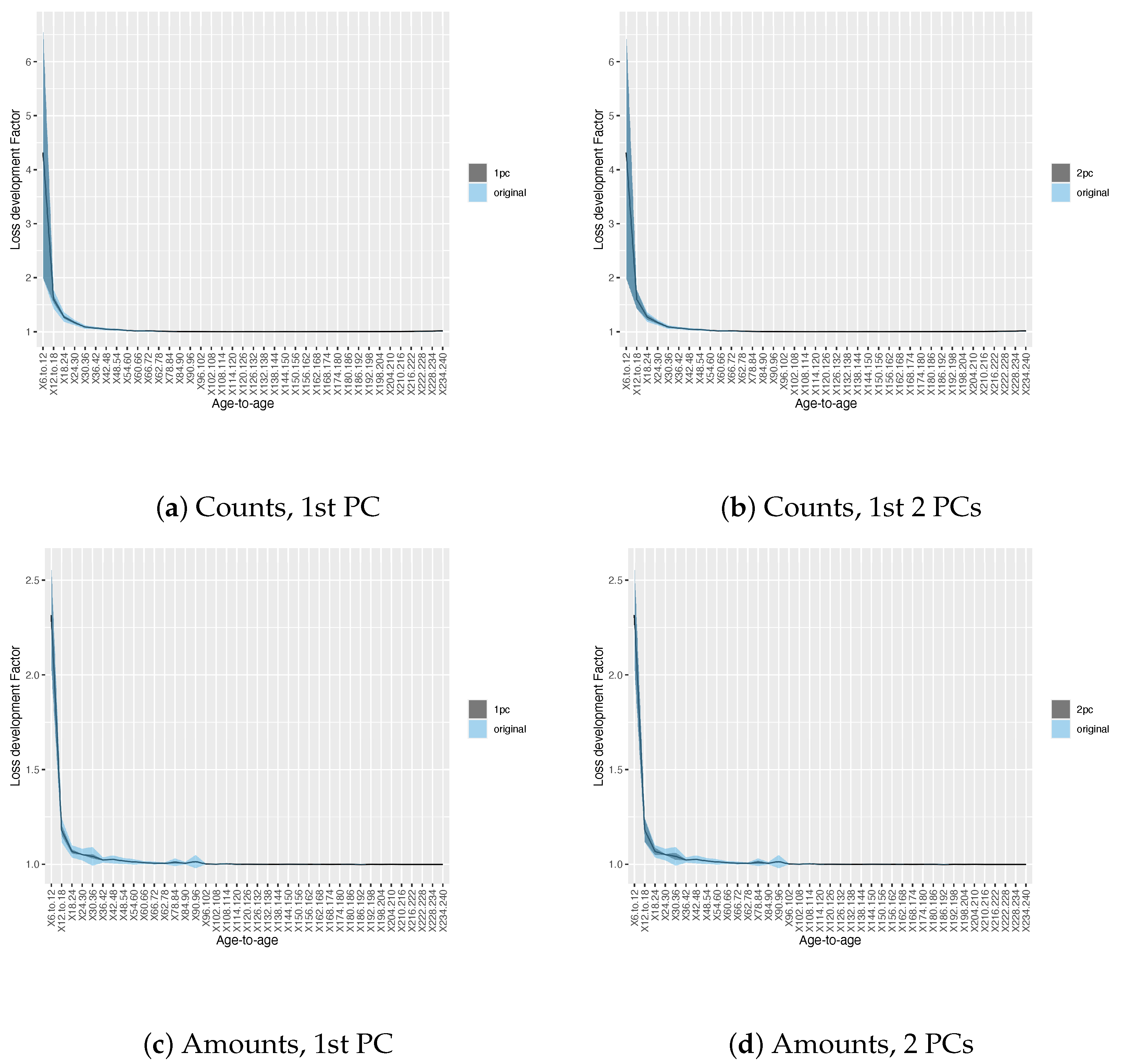
Principal Component Analysis is conducted to examine whether a small number of principal components (PCs) can effectively reduce noise while retaining the primary variability in LDFs. Figure 1, Figure 2, Figure 3 and Figure 4 present the LDFs for incurred and paid counts and losses across all development ages, for both bodily injury (BI) and medical coverages. These factors are estimated using either one or two PCs.
A consistent pattern emerges: LDFs in the first development half-year tend to exhibit higher magnitudes and greater variability, followed by a decline in both as the development age increases. This trend may be attributed to the resolution of uncertainty, where larger claims are more likely to have been settled or reserved earlier in the development period. Specifically, in medical coverage, the LDFs for incurred counts and losses initially decrease, then exhibit a temporary increase, and eventually stabilize. This mid-development increase may be due to delayed diagnosis or the late reporting of certain injuries or illnesses. However, as development progresses, the LDFs tend to converge toward one, reflecting stabilization in claim settlements and reserve development. Moreover, the LDFs estimated using either the first PC alone or the first two PCs show minimal differences and closely resemble those derived from the original data. This suggests that the first principal component captures most of the essential variation in the data and is sufficient for accurate DF estimation. The percentage of variation explained by the first and second principal components, along with their corresponding standard deviations, is reported in Table 2 and Table 3 for each major coverage, with respect to incurred loss and incurred counts, respectively.
In the plots of Figure 1, Figure 2, Figure 3 and Figure 4, the blue and grey shaded areas represent the variability of DFs across different accident years. Notably, PCA reduces the width of these intervals, particularly when using only the first PC, indicating enhanced precision in the DF estimates. This improved accuracy can support insurers in making more informed loss reserving decisions, contributing to better financial planning. From a practical standpoint, these findings suggest that PCA can effectively filter noise and highlight the dominant trend in the development patterns, which in turn enhances the reliability of reserve estimates. For insurers, this translates to more accurate and consistent reserving practices, ultimately supporting better capital management, pricing strategies, and regulatory compliance.
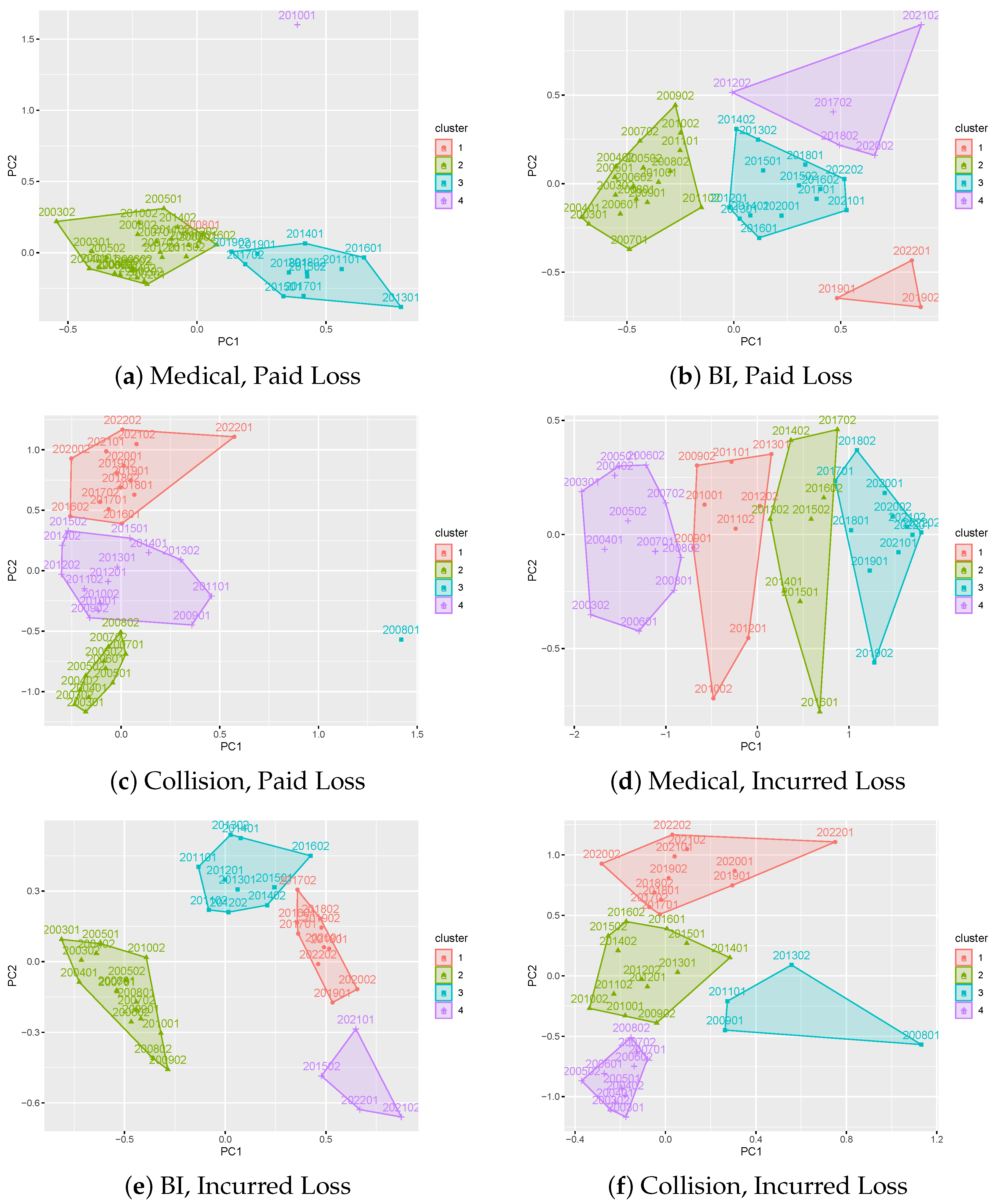
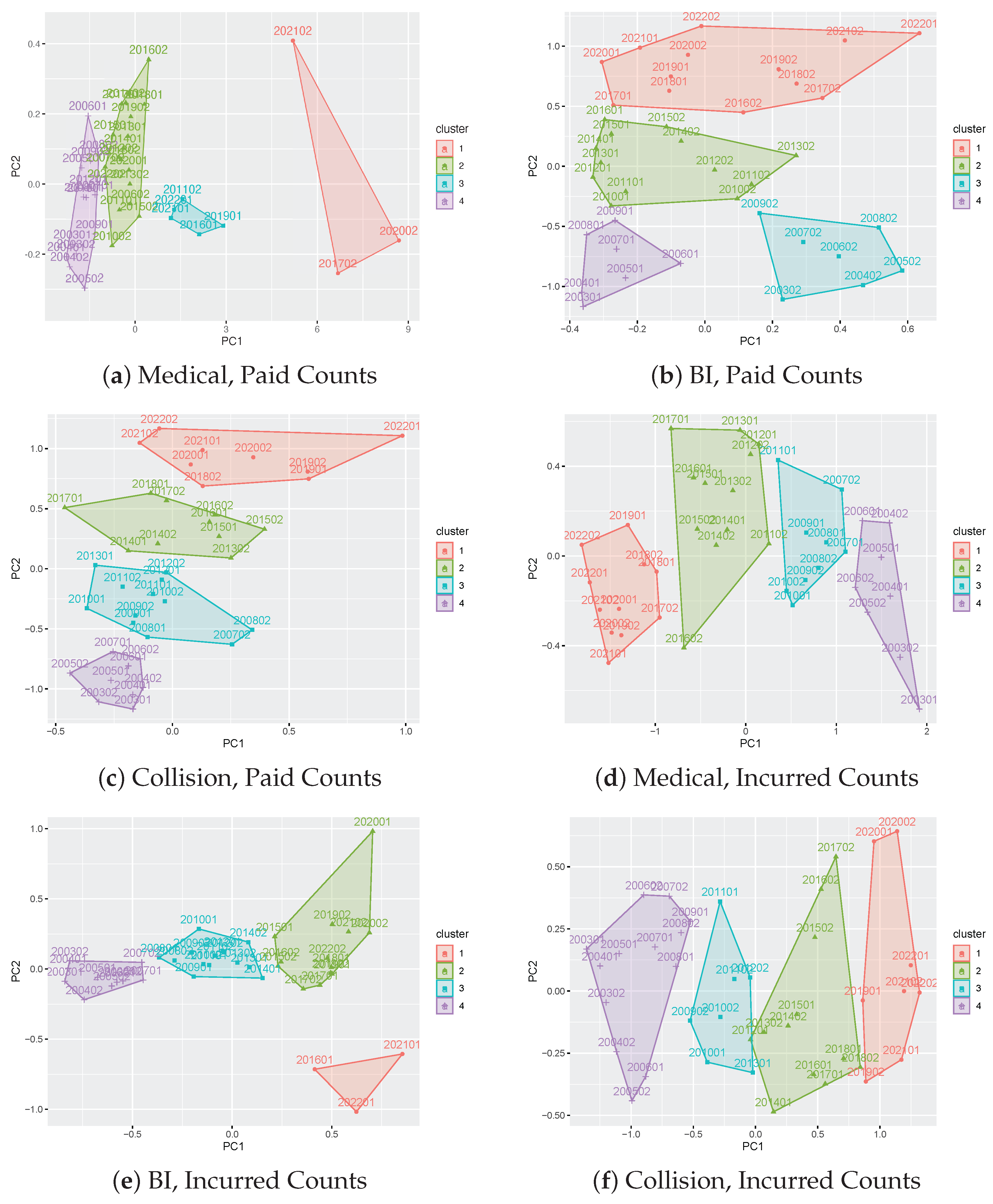
Figure 5 and Figure 6 display the first two PC scores of LDFs for incurred and paid counts and losses across medical, BI, and collision coverages. Colors represent the clusters determined using traditional K-Means clustering, while the numbers correspond to accident half-years. Interestingly, the clustering results for paid and incurred losses (Figure 5) show that cluster membership is not strictly determined by accident year. For instance, in BI coverage, the second halves of 2012, 2017, and 2020 form one cluster, while the first halves of 2013, 2016, and 2022 form another. Similar observations are made across other coverages. However, the development factors are inherently time sensitive. For example, LDFs from adjacent accident half-years may be expected to be similar, and DFs after 2019 may exhibit distinct characteristics due to the COVID-19 pandemic. To account for such temporal dependencies, we integrate accident year contiguity into our clustering approach as described in Algorithm 1.
Our proposed algorithm introduces a weight parameter w to control the influence of PC scores in clustering. We assess the contiguity of clusters (denoted C T ) for various values of w, selecting the value that minimizes C T . Once the optimal w is identified, we refine cluster memberships to improve temporal continuity. For example, in the case of incurred loss DFs for BI coverage, the minimum C T is achieved when w = 0.2 . However, with w = 0.2 , the accident half-years 201501, 201502, and 201601 are assigned to clusters 3, 4, and 3, respectively. To enhance temporal coherence, we reassign 201502 to cluster 3, aligning it with adjacent periods. This post-adjustment step ensures contiguous and practically meaningful clustering results.

3.2. Results on Development Factor Estimates

Based on the clustering results from the modified K-Means approach, we fit the data using GLM introduced in Section 2.5, for the purposes of identifying the variation contribution from different clusters and overall determining the DF estimates. The estimated DFs by group and period of incurred counts and loss, as well as paid counts and loss in three coverages, are reported in Table 4 and Table 5. For illustration purposes, only the estimates for the first five periods are listed in the main body of the paper. The tables reveal a significant group effect on the incurred loss development factors within both BI and medical coverages. When examining the temporal aspect, disparities in group effects become evident. These findings underscore the inadequacy of relying solely on single statistical measures like mean or median for age-to-age DF analysis, as they fail to capture the variability and uncertainty inherent in data across various accident years. Grouping accident years mitigates this issue, facilitating more meaningful modeling of DFs. Moreover, the observed differences among these groups point to temporal trends and variability in age-to-age DFs. Their notable distinctions emphasize that they cannot be treated uniformly. Hence, employing multiple estimates of age-to-age DFs becomes imperative, offering a dynamic perspective that captures diverse trends in reaching the ultimate DF and final estimate. This approach is essential for a comprehensive understanding of the development process.
Consistent trends emerged regarding paid losses. Significant disparities are noted in the estimations across accident year groups, highlighting the dynamic nature of age-to-age development factors. Moreover, the progression of losses for medical coverage appears temporally consistent, with fewer groups due to temporal clustering compared to other coverages. Another notable finding is the variation in group effect estimates across reporting years in our models. This suggests a dynamic pattern in loss development across different reporting years, with significant updates possibly occurring even among adjacent reporting periods. In Table 5, we observe that the claim development pattern is more time homogeneous for BI, incurred counts than the BI, paid counts. This may imply that higher variability of paid counts development pattern than the incurred counts for the BI coverage. Similar patterns are observed for the collision coverage. However, the paid counts development pattern associated with medical coverage are all volatile.
These findings have significant implications for auto insurance pricing and rate regulation practices. Understanding the group effects and temporal variability of DFs in the time domain is crucial for accurately assessing risk. By recognizing the impact of different accident years on DFs and the temporal trends therein, insurers can refine their pricing models to better reflect the evolving nature of risk. This approach allows for a more precise risk assessment of future liability, potentially leading to fairer premiums for policyholders. Moreover, regulatory bodies can utilize these insights to establish more effective rate regulations. By considering the variability and uncertainty inherent in age-to-age DFs, regulators can implement policies that ensure insurance rates remain both competitive and actuarially sound.

4. Some Discussions

This study builds upon the foundational Mack Chain Ladder model, using it to construct the development triangle that underlies our proposed analysis. From this, we form the development rectangle, a structure comprising both the observed upper triangle and a forecasted lower triangle, serving as the basis for our dimensionality reduction and clustering techniques. While the Mack model is used illustratively, our approach is model agnostic: the PCA framework can be readily applied to development rectangles generated from any reserving method, whether traditional (e.g., Bornhuetter–Ferguson) or modern (e.g., machine learning-based forecasts). By extracting dominant modes of variation across a set of projected development outcomes, PCA enables a systematic assessment of how development factors evolve, offering insights into the consistency, or disruption, of reserving assumptions over time.
Traditional chain ladder-type models typically assume that development patterns across accident half-years are identically distributed, simplifying estimation by treating these periods as replicates of a common process. However, this assumption is often violated in practice due to temporal heterogeneity induced by regulatory changes, inflation, operational shifts, or broader macroeconomic trends. To address this, we introduce a temporal clustering framework that groups accident periods based on similarity in their development trajectories. This data-driven approach relaxes the stationarity assumption and allows for the detection of structural changes in development behavior. In doing so, it supports more sophisticated reserve analysis that can adapt to evolving claims environments, thereby improving both interpretability and robustness of the estimation approaches.
Importantly, our focus is not on forecasting the unobserved lower triangle per se but rather on analyzing the variability and structural dynamics embedded within the completed development rectangle. The lower triangle is assumed to be generated by external reserving methods; we take it as given and use it as input for further analysis. Our contributions are thus exploratory and diagnostic rather than predictive in nature. Nevertheless, several limitations must be acknowledged. First, our analysis is contingent on the quality and reliability of the forecasted lower triangle; we do not assess or enhance its predictive validity. Second, the framework does not explicitly model forecast uncertainty, which may impact interpretation. Third, while the methods reveal latent structure and clustering within the data, they are not designed to produce reserve estimates or confidence intervals. Lastly, our approach presumes some level of comparability across development rectangles, an assumption that may not fully hold in the presence of significant shifts in claim handling practices or portfolio composition. Despite these limitations, our methodology offers a valuable toolkit for visualizing and interpreting complex development patterns, particularly in settings where traditional assumptions of reserving models may be under strain.

5. Conclusions

The ultimate goal of this investigation of development pattern is to estimate age-to-age development factors using observed development triangles. Our analysis employs Principal Component Analysis to investigate the variability and noise reduction of development factors. A general pattern emerges, wherein DFs exhibit higher variability and magnitude in the initial half-year, followed by a decrease as development ages progress. This trend suggests a stabilization in claim settlements and reserves over time. Moreover, the first PC proves to be sufficient in capturing the majority of information for DF estimation, with minimal differences observed when compared to DFs calculated from the original data. While clustering outcomes appear independent of accident years, the analysis underscores the necessity of considering accident years, especially in light of external factors such as the impact of COVID-19 pandemic.
Our study has shed light on the dynamic nature of age-to-age development factors in insurance claim data as evidenced by significant disparities across accident year groups and temporal variations. Through the application of principal component analysis, modified K-Means clustering and GLM, we have provided comprehensive estimates of DFs, revealing important patterns in claim development across different coverages and reporting periods. Our findings underscore the inadequacy of relying solely on single statistical measures for DF analysis and highlight the importance of using multiple estimates to capture the variability and uncertainty inherent in the loss data. These insights hold significant implications for insurance pricing and rate regulation practices, emphasizing the need for a dynamic perspective in assessing risk and ensuring fair premiums for policyholders. By recognizing and addressing the temporal trends and group effects in DFs, insurers and regulatory bodies can refine their models and policies to better reflect the evolving nature of insurance risk, ultimately promoting a more stable and equitable insurance market.

Author Contributions

Software, C.G.; Validation, S.X. and C.G.; Formal analysis, S.X. and C.G.; Visualization, S.X. and C.G. All authors have read and agreed to the published version of the manuscript.

Funding

The authors gratefully acknowledge the support of the Natural Sciences and Engineering Research Council of Canada (NSERC). This work was funded in part by an NSERC Discovery Grant.

Data Availability Statement

The data belong to the regulator and are subject to approval by the regulator. Code availability is available upon request.

Conflicts of Interest

The authors declare no conflicts of interest.

References

  1. Al-Mudafer, Muhammed Taher, Benjamin Avanzi, Greg Taylor, and Bernard Wong. 2022. Stochastic loss reserving with mixture density neural networks. Insurance: Mathematics and Economics 105: 144–74. [Google Scholar] [CrossRef]
  2. Barlak, Jan, Matus Bakon, Martin Rovnak, and Martina Mokrisova. 2022. Heat equation as a tool for outliers mitigation in run-off triangles for valuing the technical provisions in non-life insurance business. Risks 10: 171. [Google Scholar] [CrossRef]
  3. Berquist, James R., and Richard E. Sherman. 1977. Loss reserve adequacy testing: A comprehensive, systematic approach. In Proceedings of the Casualty Actuarial Society. 64 vols. Arlington: Casualty Actuarial Society, pp. 123–84. [Google Scholar]
  4. D’Arcy, Stephen P. 1987. Revisions in loss reserving techniques necessary to discount property-liability loss reserves. In PCAS LXXIV. Arlington: Casualty Actuarial Society. [Google Scholar]
  5. England, Peter D., and Richard J. Verrall. 2002. Stochastic claims reserving in general insurance. British Actuarial Journal 8: 443–518. [Google Scholar] [CrossRef]
  6. Feng, Yu Shi, and Ira Robbin. 2022. Quantifying reserve risk based on volatility in triangles of estimated ultimate losses. CAS E-Forum. Available online: https://eforum.casact.org/article/37955-quantifying-reserve-risk-based-on-volatility-in-triangles-of-estimated-ultimate-losses (accessed on 14 May 2025).
  7. Frees, Edward W., Richard A. Derrig, and Glenn Meyers. 2014. Predictive Modeling Applications in Actuarial Science. Cambridge: Cambridge University Press, vol. 1. [Google Scholar]
  8. Han, Zhongxian, and Wu-Chyuan Gau. 2008. Estimation of loss reserves with lognormal development factors. Insurance: Mathematics and Economics 42: 389–95. [Google Scholar] [CrossRef]
  9. Jeong, Himchan, and Dipak Dey. 2020. Application of a vine copula for multi-line insurance reserving. Risks 8: 111. [Google Scholar] [CrossRef]
  10. Jeong, Himchan, Hyunwoong Chang, and Emiliano A. Valdez. 2021. A non-convex regularization approach for stable estimation of loss development factors. Scandinavian Actuarial Journal 2021: 779–803. [Google Scholar] [CrossRef]
  11. Kloek, Teun. 1998. Loss development forecasting models: An econometrician’s view. Insurance: Mathematics and Economics 23: 251–61. [Google Scholar] [CrossRef]
  12. Korn, Uri. 2015. Credibility and other modeling considerations for loss development factors. CAS E-Forum, Summer 2: 1–25. [Google Scholar]
  13. Mack, Thomas. 1995. Distribution-free calculation of the standard error of chain ladder reserve estimates. Insurance Mathematics and Economics 3: 277–78. [Google Scholar] [CrossRef]
  14. Mack, Thomas. 1999. The standard error of chain ladder reserve estimates: Recursive calculation and inclusion of a tail factor. ASTIN Bulletin: The Journal of the IAA 29: 361–66. [Google Scholar] [CrossRef]
  15. Neuhaus, Walther. 2023. Consistent development patterns. Scandinavian Actuarial Journal 2023: 933–45. [Google Scholar] [CrossRef]
  16. Nugraha, Ruth Cornelia, and Danang Teguh Qoyyimi. 2022. Predicting claim reserves when the loss development factors are unstable: A case study from indonesia’s general insurance company. In International Conference on Educational Technology and Administration. Berlin/Heidelberg: Springer, pp. 109–30. [Google Scholar]
  17. Okyere Dwebeng, Daniel. 2016. Projecting Loss Reserves Using Tail Factor Development Method a Case Study of State Insurance Company (Motor Insurance). Ph.D. thesis, Kwame Nkrumah University of Science and Technology, Kumasi, Ghana. [Google Scholar]
  18. Pittarello, Gabriele, Gian Paolo Clemente, and Diego Zappa. 2022. An Individual Model for Claims Reserving Based on Bayesian Neural Networks. Technical Report. Rome: Sapienza Università di Roma. [Google Scholar]
  19. Raço, Endri, Kleida Haxhi, Etleva Llagami, and Oriana Zaçaj. 2022. Comparison of statistical methods for claims reserve estimation using r language. WSEAS Transactions on Mathematics 21: 547–52. [Google Scholar] [CrossRef]
  20. Radtke, Michael. 2016. Cape cod method. In Handbook on Loss Reserving. Berlin/Heidelberg: Springer, pp. 43–52. [Google Scholar]
  21. Sakthivel, K. M. 2016. A nonparametric approach for validation of chain ladder methods in claims reserving. International Research Journal of Engineering and Technology 3: 1616–19. [Google Scholar]
  22. Schmidt, Klaus D., and Mathias Zocher. 2007. The Bornhuetter-Ferguson Principle. Göttingen: Institut für Mathematische Stochastik. [Google Scholar]
  23. Shi, Peng, and Brian M. Hartman. 2016. Credibility in loss reserving. North American Actuarial Journal 20: 114–32. [Google Scholar] [CrossRef]
  24. Sriram, Karthik, and Peng Shi. 2021. Stochastic loss reserving: A new perspective from a dirichlet model. Journal of Risk and Insurance 88: 195–230. [Google Scholar] [CrossRef]
  25. Taylor, Gregory. 2012. Loss Reserving: An Actuarial Perspective. Berlin and Heidelberg: Springer Science & Business Media, vol. 21. [Google Scholar]
  26. Verdier, Bertrand, and Artur Klinger. 2005. Jab Chain: A Model-Based Calculation of Paid and Incurred Loss Development Factors. Zurich: ASTIN Colloquium. Available online: https://citeseerx.ist.psu.edu/document?repid=rep1&type=pdf&doi=0929a8a16a2e11377c024c3c040a383156c147b9 (accessed on 1 January 2025).
  27. Verrall, Richard J. 2000. An investigation into stochastic claims reserving models and the chain-ladder technique. Insurance: Mathematics and Economics 26: 91–99. [Google Scholar] [CrossRef]
  28. Zhao, Yixing, Rogemar Mamon, and Heng Xiong. 2021. Claim reserving for insurance contracts in line with the international financial reporting standards 17: A new paid-incurred chain approach to risk adjustments. Financial Innovation 7: 71. [Google Scholar] [CrossRef]
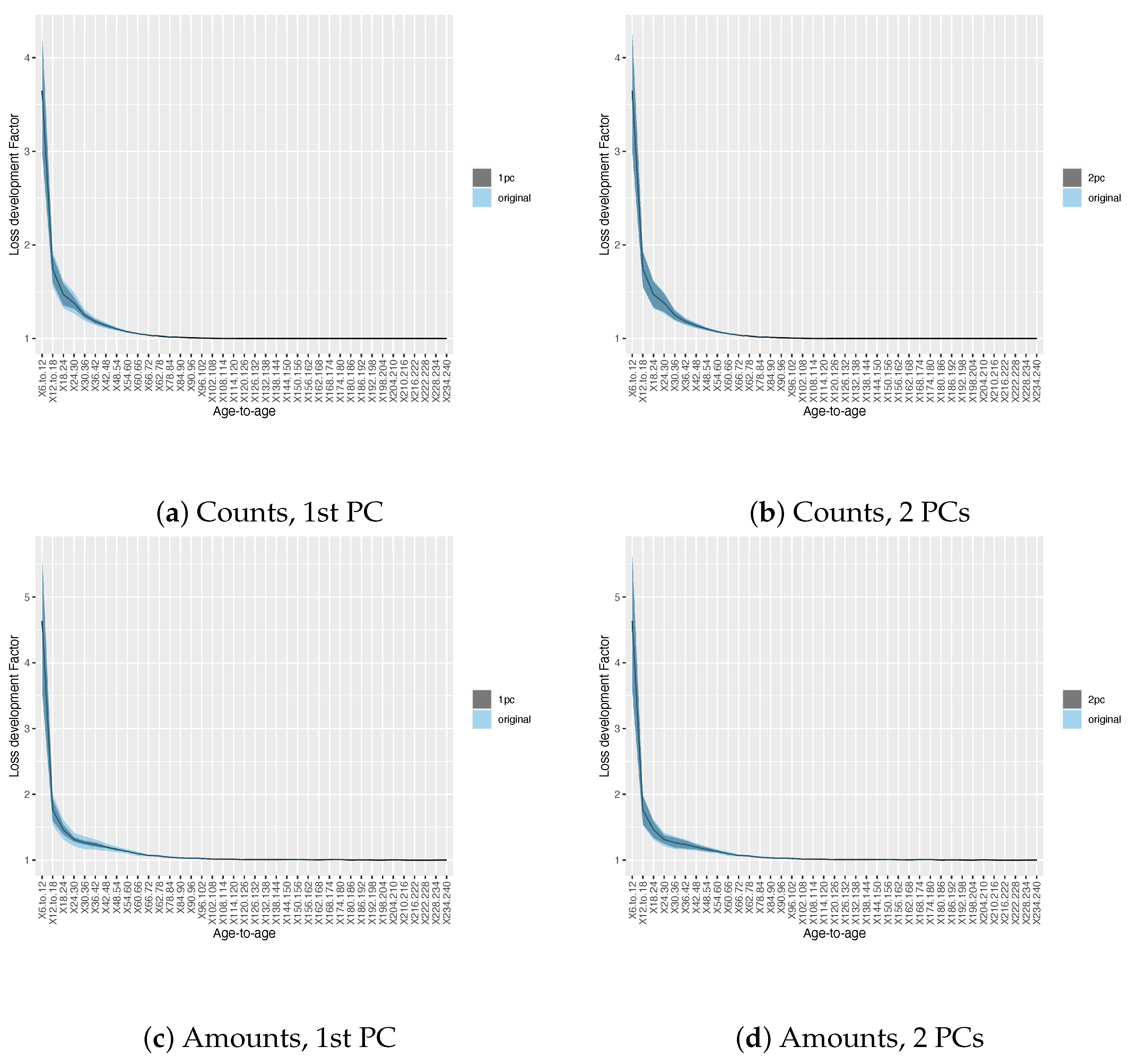
Figure 1. The functional patterns of loss development factor of incurred counts and incurred loss as a function of development age (every 6 months for up to 20 years) for Bodily Injured coverage, by different number of principal components.
Risks 13 00100 g001
Figure 2. The functional patterns of loss development factor of paid counts and paid loss as a function of development age (every 6 months for up to 20 years) for Bodily Injured coverage, by different number of principal components.
Risks 13 00100 g002aRisks 13 00100 g002b
Figure 3. The functional patterns of loss development factor of incurred counts and incurred loss as a function of development age (every 6 months for up to 20 years) for medical coverage, by different numbers of principal components.
Risks 13 00100 g003
Figure 4. The functional patterns of the loss development factor of paid counts and paid loss as a function of development age (every 6 months for up to 20 years) for medical coverage, by different number of principal components.
Risks 13 00100 g004
Figure 5. The first two principal component scores of development factor of paid loss and incurred loss respectively for medical, bodily injury and collision coverages.
Risks 13 00100 g005
Figure 6. The first two principal component scores of development factor of paid counts and incurred counts, respectively for medical, bodily injury and collision coverages.
Risks 13 00100 g006
Table 1. Illustration of a portion of age-to-age incurred loss development factors rectangle obtained from Chain Ladder under the Mack model approach for the Bodily Injury coverage. The development age is every six months, and each row represents the development of incurred losses for each accident half year (HY).
Accident HY6 to 1212 to 1818 to 2424 to 3030 to 3636 to 4242 to 4848 to 5454 to 6060 to 6666 to 72
2003012.9791.5901.2341.1781.1941.1581.2161.1451.1321.1041.067
2003023.4821.5041.3751.3181.2001.1811.2081.1691.0941.1011.062
2004013.3521.4321.2961.2851.2441.1171.1941.1511.1691.0691.077
2004023.5571.4971.4891.2741.2191.1671.1531.1911.1481.0961.102
2005013.4931.5361.3991.3461.3231.1481.1241.1311.1191.0381.052
2005024.2191.6491.4621.2441.1461.1911.2101.1491.1131.0951.075
2006013.8141.5431.3381.2281.1911.1651.2071.1681.1451.0861.074
2006024.2041.5131.3171.2861.2121.2391.1451.1141.1681.0591.057
2007013.5061.4641.3261.2551.1881.1681.1571.0951.0801.1451.076
2007023.9771.5401.2861.2311.2121.2021.2071.0931.1011.0661.075
2008013.7791.4931.3301.2991.1881.1801.1291.0791.1021.0881.063
2008024.3311.5401.2481.2051.1481.1461.1211.1341.0961.0701.062
2009013.6531.4901.3131.1791.1191.1081.1041.1191.1281.0901.066
2009024.4781.5601.2771.1511.1241.1371.1061.1271.0801.1011.040
2010013.9641.5801.2531.1631.1201.1181.1251.0841.0621.0461.062
2010023.0691.4891.2961.2381.1601.2261.1381.1241.1181.1081.095
2011014.0351.8021.6581.3061.3791.2191.2431.1681.1391.1041.080
2011024.3511.7871.4851.4041.2591.3641.2211.2391.1811.1171.116
2012014.5411.7721.7231.4971.3471.3451.1821.2131.1621.1021.073
2012024.6071.8601.3801.4291.3891.3811.2131.2561.1351.1051.052
2013014.6021.9151.6721.2051.3291.2831.2651.1781.1401.0641.058
2013024.0052.0451.3661.4651.2861.3701.2981.2171.1291.0821.057
2014014.1701.8021.6901.3781.4901.3711.2991.1901.1651.0751.059
2014025.0421.8871.5751.5761.3001.3071.3601.1961.1501.1231.090
2015015.0161.9311.6761.2301.5341.3001.2071.2411.1761.2401.093
2015027.0011.8681.4771.5161.2931.3611.2281.2261.1671.1151.074
2016015.4941.9581.5821.4851.3991.2851.3201.2041.1231.1471.085
2016025.4192.4341.4591.4201.2501.3181.2161.1631.1301.1051.083
2017015.2391.9971.5161.3111.3241.2721.2501.1611.1831.1121.091
2017024.8741.9771.6421.3911.2961.2611.2491.1671.1361.1281.072
2018015.8732.0531.6981.3151.3331.1721.1871.1781.2341.0991.072
2018025.3252.0591.5761.2281.4051.2871.1391.2371.1301.0991.072
2019015.8781.8051.6361.3351.3021.3271.2541.1611.1301.0991.072
2019025.0731.9571.5301.4041.2821.2951.1931.1611.1301.0991.072
2020015.0641.9451.4821.3711.2591.2301.1931.1611.1301.0991.072
2020026.0431.9481.7171.3231.2411.2301.1931.1611.1301.0991.072
2021016.0061.8611.5841.2871.2411.2301.1931.1611.1301.0991.072
2021027.5132.0861.4031.2871.2411.2301.1931.1611.1301.0991.072
2022016.1381.6671.4031.2871.2411.2301.1931.1611.1301.0991.072
2022024.1601.6671.4031.2871.2411.2301.1931.1611.1301.0991.072
Table 2. Standard deviation, proportion of variance and cumulative proportion of first two principle components for loss development factor of incurred and paid loss, for body injured, collision and medical coverages for the 2022 reporting year.
BI, Incurred LossCollision, Incurred LossMedical, Incurred Loss
PC1PC2PC1PC2PC1PC2
Standard deviation1.0660.2080.0300.0060.2020.066
Proportion of Variance0.9380.0360.9600.0340.7540.081
Cumulative Proportion0.9380.9740.9600.9950.7540.835
BI, Paid LossCollision, Paid LossMedical, Paid Loss
PC1PC2PC1PC2PC1PC2
Standard deviation1.2700.6700.0810.0050.2750.060
Proportion of Variance0.7540.2100.9950.0040.8780.042
Cumulative Proportion0.7540.9640.9951.0000.8780.920
Table 3. Standard deviation, proportion of variance and cumulative proportion of first two principle components for loss development factor of incurred and paid counts, for body injured, collision and medical coverages for the 2022 reporting year.
BI, Incurred CountsCollision, Incurred CountsMedical, Incurred Counts
PC1PC2PC1PC2PC1PC2
Standard deviation0.6720.1750.0610.0260.1120.052
Proportion of Variance0.9160.0620.7060.1250.5620.123
Cumulative Proportion0.9160.9770.7060.8310.5620.685
BI, Paid CountsCollision, Paid CountsMedical, Paid Counts
PC1PC2PC1PC2PC1PC2
Standard deviation0.0610.0010.1760.0262.3260.166
Proportion of Variance1.0000.0000.9640.0210.9930.005
Cumulative Proportion1.0001.0000.9640.9840.9930.998
Table 4. Loss development factor of incurred and paid loss, estimated by GLM model under Model 2: regression + group using first five periods, for body injured, collision and medical coverages from 2020 to 2022.
BI, Incurred LossCollision, Incurred LossMedical, Incurred Loss
Reported Year202020212022202020212022202020212022
group20.0210.0040.018−0.006 ***0.007 ***0.008 ***0.0770.0240.054 ***
(0.110)(0.118)(0.139)(0.002)(0.002)(0.003)(0.078)(0.020)(0.018)
group30.207 *0.195 *0.256 *−0.007 ***0.006 **0.006 **0.193 **0.106 ***0.083 ***
(0.116)(0.118)(0.131)(0.002)(0.002)(0.003)(0.076)(0.018)(0.018)
group40.450 ***0.437 ***0.556 ***0.000030.006 **0.007 ***0.132 *0.099 ***0.082 ***
(0.110)(0.108)(0.131)(0.002)(0.002)(0.003)(0.076)(0.018)(0.018)
Mean Age-to-Age DFs
Period123.9173.9734.0081.0101.0691.0711.6881.4891.518
Period182.4222.4282.4481.0020.9990.9990.9951.0261.041
Period241.8341.8321.8061.0030.9950.9950.9290.9840.997
Period301.5921.5941.5491.0030.9950.9950.9421.0041.014
Period361.3811.3761.3241.0030.9950.9950.9231.0241.035
BI, Paid LossCollision, Paid LossMedical, Paid Loss
Reported Year202020212022202020212022202020212022
group20.0860.0800.068−0.00030.022 ***0.019 ***0.073 ***0.073 ***0.073 ***
(0.071)(0.077)(0.091)(0.006)(0.007)(0.007)(0.018)(0.018)(0.018)
group30.460 ***0.455 ***0.458 ***−0.0030.0040.003
(0.071)(0.077)(0.089)(0.006)(0.007)(0.007)
group40.469 ***0.500 ***0.536 ***0.0060.0070.010
(0.071)(0.073)(0.085)(0.006)(0.007)(0.007)
Mean Age-to-Age DFs
Period124.1024.2054.3421.2181.2731.2792.2882.2882.288
Period181.4851.4801.4721.0051.0041.0041.1531.1531.153
Period241.2091.1881.1741.0010.9940.9941.0411.0411.041
Period301.0721.0491.0251.0000.9930.9931.0241.0241.024
Period361.0291.0060.9761.0000.9930.9931.0151.0151.015
Note: * p < 0.1; ** p < 0.05; *** p < 0.01.
Table 5. Loss development factor of incurred and paid counts, estimated by GLM model under Model 2: regression + group using first five periods, for body injured, collision and medical coverages from 2020 to 2022.
BI, Incurred CountsCollision, Incurred CountsMedical, Incurred Counts
Reported Year202020212022202020212022202020212022
group2−0.002−0.005−0.0070.010 *0.003−0.003−0.012−0.0100.002
(0.005)(0.004)(0.005)(0.005)(0.006)(0.006)(0.008)(0.009)(0.013)
group3−0.008−0.005−0.015−0.003−0.008−0.0090.078 ***0.071 ***−0.017
(0.005)(0.004)(0.013)(0.008)(0.008)(0.006)(0.009)(0.009)(0.012)
group4−0.003 0.00030.002−0.002−0.0050.033 ***0.035 ***0.033 **
(0.005) (0.005)(0.005)(0.005)(0.006)(0.006)(0.007)(0.013)
Mean Age-to-Age DFs
Period121.2251.2231.2271.0691.0761.0810.7540.7480.995
Period181.0111.0111.0110.9620.9650.9700.8610.8620.947
Period241.0041.0041.0040.9810.9850.9870.9710.9720.991
Period301.0031.0041.0030.9971.0021.0051.0751.0761.022
Period361.0031.0041.0030.9950.9991.0020.9650.9610.992
BI, Paid CountsCollision, Paid CountsMedical, Paid Counts
Reported Year202020212022202020212022202020212022
group20.229 ***0.234 ***0.229 ***0.0150.023 *0.0140.269 ***0.248 ***0.185
(0.045)(0.050)(0.052)(0.013)(0.013)(0.015)(0.035)(0.039)(0.205)
group30.375 ***0.370 ***0.363 ***0.024 *0.035 ***0.032 **0.359 ***0.379 ***0.429 **
(0.044)(0.049)(0.053)(0.013)(0.013)(0.015)(0.036)(0.038)(0.205)
group40.412 ***0.449 ***0.461 ***0.045 ***0.055 ***0.065 *** 0.864 ***
(0.046)(0.052)(0.051)(0.013)(0.013)(0.016) (0.200)
Mean Age-to-Age DFs
Period123.1963.3093.3831.6681.6721.6883.0953.1803.925
Period181.4201.4491.4761.0611.0591.0611.4641.5071.212
Period241.1621.1781.2051.0131.0101.0121.2331.2620.881
Period301.0851.0971.1151.0000.9960.9971.1541.1780.778
Period360.9730.9750.9840.9930.9880.9891.0311.0410.696
Note: * p < 0.1; ** p < 0.05; *** p < 0.01.
Disclaimer/Publisher’s Note: The statements, opinions and data contained in all publications are solely those of the individual author(s) and contributor(s) and not of MDPI and/or the editor(s). MDPI and/or the editor(s) disclaim responsibility for any injury to people or property resulting from any ideas, methods, instructions or products referred to in the content.