Abstract
Volatility forecasting for financial institutions plays a pivotal role across a wide range of domains, such as risk management, option pricing, and market making. For instance, banks can incorporate volatility forecasts into stress testing frameworks to ensure they are holding sufficient capital during extreme market conditions. However, volatility forecasting is challenging because volatility can only be estimated, and different factors influence volatility, ranging from macroeconomic indicators to investor sentiments. While recent works show promising advances in machine learning and artificial intelligence for volatility forecasting, a comprehensive assessment of current statistical and learning-based methods is lacking. Thus, this paper aims to provide a comprehensive survey of the historical evolution of volatility forecasting with a comparative benchmark of key landmark models, such as implied volatility, GARCH, LSTM, and Transformer. We open-source our benchmark code to further research in learning-based methods for volatility forecasting.
1. Introduction
Risk management is essential to financial institutions because it is required by regulators and highly relevant to their performance. An integral aspect of this risk stems from the movement of the equity market, especially the market’s volatility. Volatility can be used to determine the risk exposure of a portfolio (R. Engle 2004), the anticipated fluctuations throughout the duration of an option (Black and Scholes 1973), and the bid–ask spread of options as well as their underlying asset (Bollerslev and Melvin 1994). A model that helps financial institutions forecast the volatility of their holdings would provide a clearer picture of their risk and facilitate the process of risk management and decision-making.
Volatility cannot be observed; therefore, it has to be estimated, which is why we embark on this journey to survey different volatility models. There are various ways that researchers have used to estimate volatility; the two most common ones are realized volatility, which is the annualized standard deviation of log returns, and implied volatility, which is a forward-looking metric calculated from options. While the Black–Scholes model as the basis of implied volatility has unrealistic assumptions, it is based on actual market data and has been a standardized way of quantifying volatility. In this paper, we choose realized volatility as our prediction target and use implied volatility as one of the ways to predict it. Other than implied volatility, researchers have employed a wide range of other models, ranging from traditional Generalized Autoregressive Conditional Heteroskedasticity (GARCH) (Bollerslev 1986) to Neural Network frameworks such as Long Short Term Memory (LSTM) (Hochreiter and Schmidhuber 1997) and transformers (Vaswani et al. 2023). In this paper, we compare the relative performance of these models, showing how machine learning models have significantly outperformed earlier ones, while also discussing the limitations of these models, some of which are hard to interpret intuitively.
Volatility exhibits a series of stylized facts, including temporal clustering (Mandelbrot 1997; Kim and Shin 2023), long memory (Poon and Granger 2003), heavy tails (Cont 2001), leverage effect (McAleer and Medeiros 2008; Aıt-Sahalia 2017; Engle and Ng 1993; Tversky and Kahneman 1991; Christie 1982; Bekaert and Wu 2000), and mean reversion (Goudarzi 2013). These stylized attributes make volatility forecasting possible and are detailed in Appendix A. Nevertheless, predicting volatility remains a challenging endeavor. Volatility is influenced by a wide range of factors, including macroeconomic phenomena, corporate earnings reports, interest rates, global commodity price trends, and psychology (Shiller 1999). The interactions among these factors can be complex. Volatility as a proxy for risk is easily mistaken for uncertainty (Knight 1921). Volatility can be estimated when one knows the range of possible outcomes and can thus assign a probability distribution to these outcomes—in other words, measurable unknowns. Uncertainty, by contrast, refers to unknown unknowns, and, hence, no probability distribution can be assigned to these unknown outcomes. Examples include exogenous shocks, such as geopolitical tensions, natural calamities, or abrupt regulatory shifts, which can yield immediate and pronounced volatility spikes and are inherently challenging to anticipate.
The benefits and challenges of forecasting volatility have garnered attention from many, and ongoing revisions have been undertaken to include the latest developments in this domain (Andersen et al. 2005). There are numerous studies surveying volatility forecasting methods (Ge et al. 2023; Sezer et al. 2020); however, they either focus on a specific type of model or do not incorporate the current state-of-the-art models. We are not aware of a recent comprehensive review that provides a clear explanation and compares the foundational and cutting-edge volatility models side by side. Within this paper, we survey the evolution of volatility forecasting models and evaluate their performance using a representative dataset from the Standard and Poor’s 500 index (S&P 500). Section 2 provides a comprehensive literature review; Section 3 discusses the models we used and their advantages and disadvantages. Section 4 discusses how the models perform during extreme periods of market volatility, like the 2008 Financial Crisis and the 2020 COVID-19 Pandemic. Section 5 illustrates the results, and Section 6 discusses the implications of these results. Section 7 provides a conclusion, and Section 8 provides some future work directions. The contributions of this paper are as follows:
- We survey the evolution of volatility forecasting models, transitioning from traditional AR and implied volatility models to contemporary variations of the transformer models representing the current state of the art.
- We select a representative model from each category and conduct a systematic review to show their respective performances, paving the way for subsequent model developments.
- We open-source our analysis framework and highlight the advantages and disadvantages inherent to each type of model.
2. Literature Review
2.1. Overview
In volatility forecasting, numerous models have been employed, and many of them have been applied in conjunction with others. We selected models that are well documented in papers. Given the extensive nature of research in this field, we focused on those related to volatility forecasting, validated by multiple datasets, and made an important paradigm shift. For organizational purposes, we have categorized these models into four primary classifications: statistical models, implied volatility, recurrent neural networks (RNNs) (Connor et al. 1994; Chung et al. 2014), and transformers, as detailed in Figure 1. In the following sections, we first examine each category and its models. Then, we discuss the advantages that led to the emergence of each and their limitations. Finally, we highlight the landmark models within these categories and perform a comparative analysis.
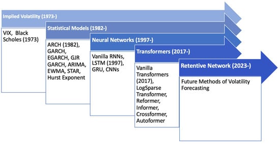
Figure 1.
Timeline for the evolution of volatility prediction models.
2.2. Implied Volatility
The Chicago Board Options Exchange’s CBOE Volatility Index (VIX) and implied volatility (IV) are widely used as predictors for future volatility. Often referred to as the “fear index”, the VIX mirrors the market’s 30-day anticipated volatility (Whaley 2009). Unlike its original derivation, which was based on a narrow set of strike prices to determine implied volatility, today, the VIX is based on the methodology of a volatility swap (Derman 1999). However, rather than being an actual swap, a volatility swap is a forward contract on the realized variance (Diamond 2012). The computation of VIX uses two months of the latest option data while interpolating between the nearest and second nearest expiration months to create a consistent 30-day window of expected volatility. Specific option strikes are then chosen for the VIX calculation, as elaborated in the VIX white paper (CBOE 2019). IV is viewed as a reliable predictor because it reflects actual investor expectations (Poon and Granger 2003). However, IV has its limitations. It can only be estimated through an iterative procedure using option prices.
2.3. Statistical Models
To address the stylized facts, Robert Engle’s Autoregressive Conditional Heteroskedasticity (ARCH) model (R. F. Engle 1982) was initially adopted for volatility forecasting. This was followed by the introduction of the Generalized Autoregressive Conditional Heteroskedasticity (GARCH) model by his student Tim Bollerslev, with the common goal of leveraging the occurrence of volatility clustering (Andersen 2018). Since its inception, numerous scholars have employed and adapted the GARCH model. For example, the asymmetric GARCH (AGARCH), Exponential GARCH (EGARCH), and Glosten Jagannathan Runkle GARCH (GJR GARCH) observed that negative shocks have a more substantial impact on the variance than positive shocks. According to the survey paper Bollerslev wrote in 2008 (Bollerslev 2008), there were already numerous variants of the original ARCH model, and this number is continuously growing. Other than GARCH models, other statistical models include the simple moving average (SMA) (Johnston et al. 1999), exponentially weighted moving average (EWMA) (Holt 2004), Smooth Transition Exponential Smoothing (Taylor 2004), autoregressive integrated moving average (ARIMA) (Box and Pierce 1970), and smooth transition autoregressive (STAR) (Bildirici and Ersin 2015). These models accommodate factors such as seasonality, long-term trends, autoregressive, and moving averages. Among them, SMA creates a smooth curve from past data over a defined period, while EWMA emphasizes recent data more by giving more weight to recent observations. The Smooth Transition Exponential Smoothing model uses a logistic function based on a selected variable for its smoothing effect. ARIMA combines autoregressive techniques and moving averages, and STAR focuses on detecting nonlinear trends in data.
A common characteristic among AR models is their reliance on historical values and stationarity for predictions. For a time series to be stationary, its statistical properties, such as mean, variance, and covariance, must not be a function of time. To test whether a time series is stationary, the Augmented Dickey–Fuller (ADF) test is typically implemented. Stock prices themselves are not stationary, as they tend to increase with a drift term; however, their log returns are usually stationary. The requirement of converting price data to log return data is a significant limitation for AR models when implemented in real-time. Volatility time series generally require treatment to become stationary, and the specific treatment depends on whether the time series is deterministic. A deterministic series means the same input generates the same output every time, whereas a stochastic series produces different results. While there are deterministic patterns in volatility, such as long-term mean reversion and volatility clustering, a significant portion of volatility arises from uncertainty, as discussed in the introduction. Although chaos theory suggests an alternative explanation that volatility is deterministic yet highly sensitive to initial conditions, stochastic models like the Heston, GARCH, and SABR models are widely used. The detrending and differencing methods aim to remove the trend and seasonality from the time series and focus on the stochastic part instead. In general, detrending removes the trend from the time series, a technique that can be applied if the volatility is deterministic. Differencing, which is subtracting the previous observation from the current one, is more appropriate for stochastic cases. They were both widely adopted in statistical and machine learning models (Raudys and Goldstein 2022; Granger and Joyeux 1980). If the underlying data are non-stationary, there are alternative methods such as the Hurst Exponent, which measures whether the trend shows momentum or is mean reverting (Hurst 1951; Qian and Rasheed 2004).
2.4. Tree-Based Models and PCA
With its ability to learn from and make predictions based on data, machine learning has been applied to more and more fields, and finance is no exception. Unlike econometric models that aim to be parsimonious by limiting the number of parameters, machine learning embraces the use of a vast number of parameters (Kelly and Xiu 2023). This approach has led to the adoption of many new techniques for volatility forecasting, either as entirely new methods or as extensions of existing ones. The following paragraphs will start with traditional machine learning (ML) models and extend to neural networks (NNs), both used extensively for volatility analysis.
Decision trees (DTs) (Loh 2011), random forests (RF) (Breiman 2001), and XGBoost (Chen and Guestrin 2016) are among the foundational applications for machine learning. Decision trees consist of a supervised learning algorithm that ascertains the value of a target variable by deducing straightforward decision rules from the data’s features. The Random Forest (RF) algorithm operates as an ensemble of these decision trees, chosen through stochastic processes. XGBoost is an optimized distributed gradient boosting library rooted in decision tree algorithms (Zhang et al. 2023). Different from random forest, XGBoost uses a boosting method to combine trees together so that each tree corrects the error of the previous one.
Furthermore, another well-used machine learning model is Principal Component Analysis (PCA). PCA reduces the dimension of the dataset while ensuring the principal components are still consistent estimators of the true factors (Stock and Watson 2002). For example, Ludvigson and Ng found a volatility factor and a risk premium factor that contain significant information about future returns (Ludvigson and Ng 2007). Such analysis is further improved by assigning weights to predictors that reflect their relative forecasting strength (Huang et al. 2022).
2.5. Neural Networks
While traditional ML methods performed well in short-term forecasting, they also have several limitations. Their ability to predict long-term and complex volatility is limited, and missing values, which are not uncommon in practice, can cause significant issues for these traditional models. In order to address these problems, neural networks (NNs) were introduced (Pranav and Hegde 2021). NNs were inspired by the biological neural networks in human brains and can detect complex patterns in nonlinear form (Hornik et al. 1989). Structurally, a neural network (NN) is composed of multiple layers. Each layer features neurons that are interconnected through weighted links, which are then adjusted during the training process. This adjustment is done by using backpropagation to compute the gradient of the loss function for each weight using the chain rule.
NNs were traditionally used for tasks like image and speech recognition (Abdel-Hamid et al. 2014), targeted marketing (Venugopal and Baets 1994), and autonomous vehicles (Pomerleau 1988). When applied to time series, the NNs can recognize the relationship between past and current inputs and use them to predict future outputs. While various NNs have been applied (Chow and Leung 1996; Marcek 2018), recurrent neural networks (RNNs) are particularly prominent for time series-related tasks. RNNs use activation functions to model nonlinear relationships. They will retain information specific to a particular timestep and sequentially update it at each future step. This makes them ideal for time series analysis. In the RNN process, data are initially fed to produce a preliminary result. This result is then contrasted with the actual outcome using the loss function. Subsequently, backpropagation will be used to fine-tune the gradient for each neuron in the network. This iterative process optimizes each neuron’s weight. However, despite their potential, RNNs have limitations, especially the vanishing gradient problem (“Gradient Flow in Recurrent Nets: The Difficulty of Learning LongTerm Dependencies” Kolen and Kremer 2009). In backpropagation, derivatives are calculated layer by layer from the end to the beginning. As per the chain rule, when these derivatives are successively multiplied, they can diminish exponentially, causing them to vanish. Similarly, the gradient could also explode if the opposite happens. These lead to the RNN’s failure to learn long-term dependencies. RNNs are also computationally expensive and cannot be parallelized, which makes training an RNN difficult.
Algorithmic methods such as Long Short Term Memory (LSTM) and Gated Recurrent Unit (GRU) have been introduced to address these problems. Both LSTM and GRU extend the capabilities of RNNs. These models employ gates to update or remove information to the hidden states to address the long-term dependencies. The GRU is a simplified version of the LSTM that combines and reduces parameters. While less powerful, it is relatively faster compared with LSTM. Both LSTM and GRU are widely used in time series forecasting, both on their own and in conjunction with other models (Kim and Won 2018; Ozdemir et al. 2022; Gu et al. 2020). However, the sequential nature of LSTMs and GRUs makes them time-intensive when working with larger data.
Another neural network used is Convolutional Neural Networks (CNNs), which was widely used in computer vision for image recognition tasks. Using CNNs would require image format data, which can be achieved in different ways, such as snapshots of data in a bounded period (Gudelek et al. 2017) or multiple technical indicators, each with the same length (Sezer and Ozbayoglu 2018).
2.6. Transformers
Transformers address the problems of RNNs by taking advantage of GPUs to do parallel computing. The original use of a transformer was in translating languages, but soon it saw extensive use in different tasks like audio processing (Huang et al. 2018), computer visions (Liu et al. 2021), and time series (Ahmed et al. 2022; Zerveas et al. 2021). Transformers abandon recurrence entirely and use the attention mechanisms instead. Transformers have an encoder–decoder structure. The encoder maps the input sequence and produces a continuous representation, and the decoder chooses what and how much previously encoded information to access. The encoder’s attention mechanism derives attention scores from input vectors of queries, keys, and values. These scores determine the weight of each piece of information in predicting every time step. A dot product was used for simplicity in the original transformer model, whereas many different approaches were introduced in later works (Wen et al. 2023). To further refine and simplify the process, an array of attention mechanisms emerged.
Notable examples include the LogSparse Transformer (Li et al. 2019), Reformer (Kitaev et al. 2020), Informer (Zhou et al. 2021), Crossformer (Zhang and Yan 2023), and Autoformer (Wu et al. 2021). As research in this area is ongoing, these mechanisms constantly advance the state of the art. In their distinct ways, these innovative mechanisms cut time and memory requirements compared to the original transformer.
The LogSparse Transformer introduces convolutional self-attention. It generates queries and keys using causal convolution, prioritizing more recent information for immediate step forecasting. The Reformer uses locality-sensitive hashing to replace simple dot products and reversible residual layers to replace standard residuals. The Informer shares similarities with LogSparse by utilizing the sparsity found in the self-attention probability distribution. However, the Informer identifies a long-tail distribution within the attention distribution. Therefore, it leverages the fact that a small number of dot products produce the majority of attention to selectively choose only the top queries and replaces vanilla self-attention with ProbSparse self-attention. The Crossformer identifies a gap in cross-dimensional dependency modeling. To remedy this, it introduces a Two-Stage Attention (TSA) layer to bridge this deficiency. Autoformer model utilizes a decomposition layer to separate the time series into long-term trends, seasonality, and random components. Then, it replaces the self-attention with the autocorrelation mechanism, which extracts frequency-based dependencies from queries and keys instead of the vanilla dot product.
Despite transformers being regarded as a state-of-the-art (SOTA) way of forecasting volatility, Zeng et al. (2023) challenged this notion by introducing a straightforward single-layer linear model that surpassed all current transformer models across nine datasets. They argued that transformer architectures, despite their success in NLP, may not be suitable for time series forecasting. This suggests that the self-attention mechanism is inherently anti-order. Zeng argued that while this might not significantly impact sentences, as they retain most of their meaning even if the sequence of the words is changed, it is problematic for time series where the continuous sequence order is vital.
This perspective quickly gained attention. For instance, Nie et al. introduced PatchTST (Nie et al. 2023), addressing the anti-order issue by segmenting time steps into subseries-level patches. Although Cirstea et al. (2022) first introduced the concept of patches for simplifying complexities, PatchTST was the first to utilize them as input units. Furthermore, they incorporated a channel-independence technique previously validated by Zheng et al. (2014). This ensures the input token is derived from a single channel, in contrast to earlier transformers that adopted channel-mixing methods. Their results indicated a marked improvement over both standard transformers and the linear model proposed by Zeng et al. (2023). Other than ignoring the temporal dependencies, the transformer also faces common shortcomings that many models face, such as being prone to overfitting, dependency on stationarity, and hard to interpret. Additionally, they are computationally intensive, memory-demanding, and prone to high latency when deployed in real-time applications, highlighting the need for further refinement and optimization.
While constructing the paper, Microsoft and Tsinghua University introduced a novel architecture called the Retentive Network (Sun et al. 2023). This architecture is presented as an enhancement to the Transformer model, which reduces inference costs and long-sequence memory complexity. Although its primary intention is for use in language models, similar to the evolution of transformers, this architecture may find broader applications, like time series.
2.7. Hybrid and Ensemble Models
While statistical models like EWMA and GARCH differ from neural networks, they still share many similarities that make hybrid designs possible (Kim and Won 2018). For example, the GARCH model can be viewed as an RNN without the output layer and activation functions (Zhao et al. 2024). Among the hybrid models, the most notable one is GARCH-LSTM, where GARCH’s output replaces the output gate of LSTM, and the GARCH parameters are used as features in the LSTM network (García-Medina and Aguayo-Moreno 2024). Various types of GARCH LSTM models have shown performance improvement, and the GARCH model adds valuable input to the NNs. For example, Koo and Kim developed a volume-up method to avoid biases in the input distribution and improve the result. They compared their VU strategy with ten different GARCH-LSTM variants, such as EGARCH with LSTM (Koo and Kim 2022). Another hybrid model is GARCH-MIDAS (Mixed Data Sampling), which keeps the GARCH process for the short term and uses macroeconomic variables as part of the long-term component (Asgharian et al. 2013; Fang et al. 2020). Ensemble models also show performance improvement. For example, He et al. proposed an ensemble model based on CNN, LSTM, and ARMA that improved accuracy and robustness compared with individual models (He et al. 2023). Olorunnimbe and Viktor used an ensemble of temporal transformers and showed a 40% to 60% improvement over the baseline temporal transformer (Olorunnimbe and Viktor 2024).
3. Methods
3.1. Overview
We will discuss four milestone models: Generalized Autoregressive Conditional Heteroskedasticity, implied volatility, Long Short Term Memory, and transformer. Table 1 summarizes the advantages and disadvantages of each model. We selected these four models because they are representative of each of the categories we discussed and are widely used. We aim to trace the historical evolution of volatility forecasting techniques by showing how newer models compare to earlier ones. In the following section, we show the methodology of each model. We used Python 3 to implement these models and tested their performance when used to forecast volatility. We evaluate their performance based on root mean square error (RMSE), which is a widely used metric for predicting numerical data.

Table 1.
Summary of the advantages and disadvantages of the different models.
3.2. Data Processing
We used thirty years of daily S&P 500 data from Yahoo Finance, 1 October 1993 to 1 October 2023. We used the first twenty-eight years for training and the last two years for testing, as shown in Figure 2. The actual training data (3 December 1993 to 28 September 2021) is slightly shorter than twenty-eight years because of data loss when processing data and calculating rolling returns. We calculated the realized volatility as the annualized standard deviation of 22 rolling trading days’ (as an approximation for one month in time) log return. We also tried 11 trading days (approximately 15 days), and the RMSPE for GARCH and IV are relatively stable but nearly doubled for the transformer and tripled for LSTM, at 0.10 and 0.14, respectively. The logarithmic return for a given day t is represented as follows:
where:
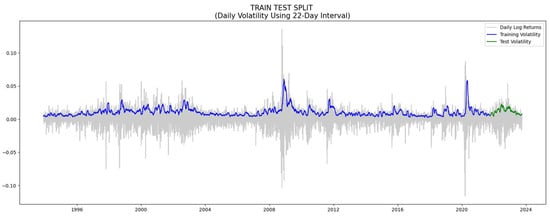
Figure 2.
Training and testing data intervals.
- rt: Log return on day t.
- Pt: Price on day t.
- Pt−1: Price on the previous day, day t − 1.
The average log return over 22 trading days is as follows:
The realized volatility over 22 trading days is given as follows:
3.3. Implied Volatility
What distinguishes IV from other models is that it is forward-looking. Implied volatility captures the market’s expectation of the volatility for the next 22 trading days, calculated backward from the option’s price using the Black Scholes Merton Formula:
where:
Explanation of terms:
- c: Price of the European call option.
- p: Price of the European put option.
- S0: Current stock price.
- K: Strike price of the option.
- T: Time to maturity (in years).
- r: Risk-free rate.
- q: Continuous dividend yield.
- N(.): The probability that a variable with a standard normal distribution will be less than x.
- σ: The standard deviation of the stock’s returns.
While it is impossible to invert the function to calculate implied volatility directly as a function of other variables, an iterative approach can be used to search for implied volatility (Hull 2018). In this paper, we used the corresponding daily close of the VIX index as the implied volatility and compared it with the realized volatility of the S&P 500. The VIX data are available from the Chicago Board Options Exchange (CBOE).
3.4. GARCH
The ARCH model was introduced prior to the GARCH model for forecasting volatility. The name, Autoregressive Conditional Heteroskedasticity, means that volatility depends on the time series value in previous periods and some error terms. GARCH is a variant of the ARCH model that addresses the problem of predictions being bursty, which means the predictions vary by a huge amount day by day. This enhancement is achieved by taking the previous day’s volatility into the current day’s calculation, alongside the ARCH model’s time series value and error term. The equation for GARCH(p, q) is as follows:
where:
- : Conditional volatility at time t.
- α0: positive empirical parameters.
- αi: Non-negative empirical parameters.
- : the squared residual at time t − i.
- : Non-negative empirical parameters.
- : Variance of the return series at time t − j.
While there are many different versions of GARCH models, we used a simple GARCH (1,1) model, as this model is representative, simple, and powerful (Hansen and Lunde 2005). GARCH (1,1) considers only one lag of the squared return and one lag of the conditional variance. The equation for the GARCH (1,1) model is as follows:
We used rolling forecast techniques, and the model used the training data as well as the past test data.
3.5. LSTM
The equations for LSTM are as follows:
The cell state (C):
The forget gate (f):
The input gate (i):
The output gate (o):
The hidden state ht:
The candidate for cell state at timestamp t ():
where
- σ: sigmoid activation function.
- Wf, Wi, WC, and Wo: weight matrices for the forget gate, input gate, candidate values, and output gate, respectively.
- bf, bi, bC, and bo: biases corresponding to each gate.
- ht−1: last hidden state.
- xt: current input.
- tanh is the hyperbolic tangent activation function.
Our model used a 22-day windowed dataset, and we performed a hyperparameter search using Keras Random Search with 20 trials to optimize our results. Our hyperparameter search results suggest a two-layered bidirectional LSTM model with 128 and 32 units. We used 200 epochs with a batch size of 32 to train the LSTM model. We applied a dropout rate of 0.2 to reduce overfitting. We used bidirectional LSTM because it retains forward and backward sequence information, which helps the model better understand the context—a crucial aspect in forecasting volatility. We used the Adam optimizer to optimize our model, employed an early stopping with a patience level of 20, and only kept the best model. A visual for the LSTM architecture is shown in Figure 3. The details for the LSTM model are shown in Appendix B.
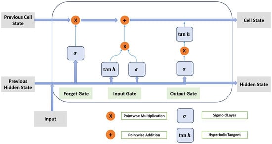
Figure 3.
Long Short Term Memory.
3.6. Transformer
We built a vanilla transformer that is modified to work with time series tasks. We processed our data in batches of 32 over 200 epochs. During preprocessing, we windowed our dataset into 22-day segments and reshaped it into three dimensions. The details for the transformer model are shown in Appendix C.
We performed a hyperparameter search and set the hidden layer size to be 16, dropout to be 0.1, and the number of units in the multilayer perceptron (MLP) layer to be 256. We used 4 layers for our encoder. Each layer contains Layer Normalization, Multi-Head Attention, dropout, Residual Connection, and a feed-forward network. Figure 4 shows a visual for Multi-Head Attention. The equation for Multi-Head Attention is as follows:
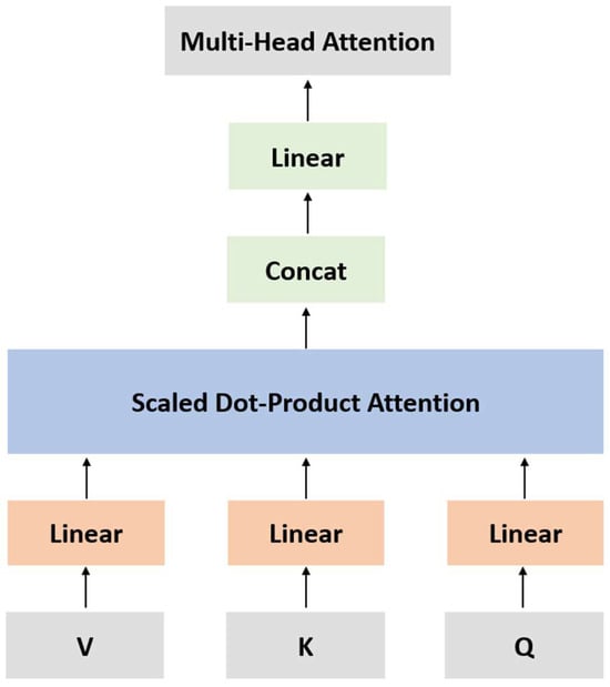
Figure 4.
Multi-Head Attention (transformer).
3.7. Evaluation Metrics
To compute for errors, we used mean absolute error (MAE), root mean square error (RMSE), and root mean square percentage error (RMSPE):
where
- N: Total number of observations.
- Ai: Actual value for the ith observation.
- Fi: Predicted value for the ith observation.
4. Performance During Crisis Periods
4.1. Overview
We selected two recent crisis periods to test the models’ performance during extreme scenarios where volatility spikes: the 2008 Financial Crisis and the 2020 COVID-19 Pandemic. We kept the other parameters in the models unchanged except for using different periods of training and testing data for each case. As demonstrated in the table below, LSTM showed slightly better performance than the transformer overall, while both outperformed the GARCH and IV models. All numerical results are shown in Table 2, and the baseline visual is shown in Figure 5.
Table 2.
Comparison of different models’ performance (the best performing model is bolded).
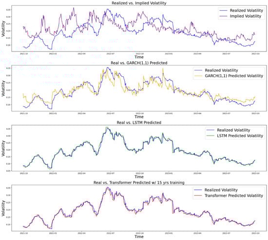
Figure 5.
Comparison of performance (base scenario: training from 3 December 1993 to 28 September 2021).
4.2. 2008 Financial Crisis
We used a training period from 3 February 1997 to 8 February 2007 and a testing period from 9 February 2007 to 9 February 2009. The results are shown in Figure 6.
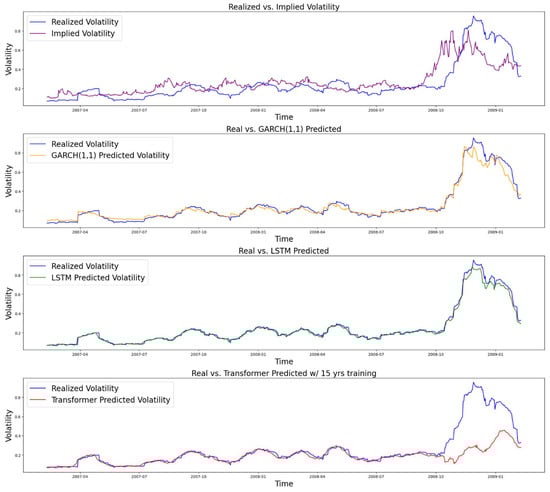
Figure 6.
Comparison of performance (Financial Crisis period: training from 3 February 1997 to 8 February 2007).
4.3. 2020 COVID-19 Pandemic
We used two different data periods for the training part of the COVID-19 case to compare the performance of machine learning models when given different lengths of training data. Specifically, we selected two periods: one that does not include the 2008 Financial Crisis, and another that does. The first period uses data from 1 March 2010 to 3 March 2020 for training and from 4 March 2020 to 2 March 2022 for testing. The second period uses data from 25 February 2005 to 3 March 2020 for training and from 4 March 2020 to 2 March 2022 for testing. We refer to the two datasets as COVID10 and COVID15, respectively. The results are shown in Figure 7 and Figure 8, respectively.
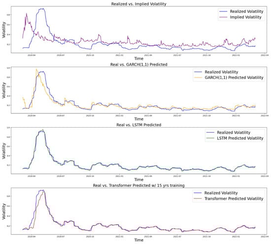
Figure 7.
Comparison of performance (COVID with 10 years of training: from 1 March 2010 to 3 March 2020).
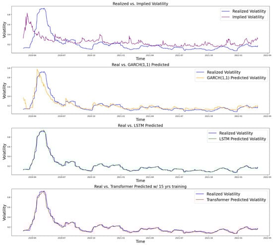
Figure 8.
Comparison of performance (COVID with 15 years of training: from 25 February 2005 to 3 March 2020).
5. Results
As our goal is to forecast future market volatility, the value we are trying to predict is the realized volatility in the future. To compare the performance of our models, we calculate both the RMSE and the RMSPE between the model prediction and the target. We used historical VIX close value, which makes the computation faster than what would happen intraday in real-time, which is updated every 15 s.
In the thirty years of S&P 500 data we used to train and test our models, the LSTM and transformer models significantly outperformed the econometrics models, such as GARCH. Among these two models, the older LSTM performed slightly better with an RMSE of 0.010, while the transformer had an RMSE of 0.011. The results are shown in Table 2 and Figure 5. In Section 4, we conducted comparative studies to show how models perform when fewer data are given and when extreme events occur, like the 2008 Financial Crisis and the COVID-19 pandemic. While the LSTM model still outperforms, the transformer model’s performance drops significantly, mainly due to the requirement for a large amount of training data. This is most evident when testing during the financial crisis period of 2008 (Figure 6). The relatively short period of training data did not include a comparable period where stock prices were as volatile as they were in the financial crisis, and the transformer model failed to capture the sudden increase in volatility. As the LSTM model performs the best, we also tested similar models, such as GRU and RNN, which are simplified versions of the LSTM. They both performed reasonably well with an RMSE of 0.018 and 0.017, respectively, while there is still a significant gap compared with LSTM. We include the details for these two models in Appendix D.
To ensure universality and fairness in comparison, we constructed models for each category that are general and representative instead of fine-tuned for specific tasks. While these models provide an adequate representation for the purpose of this benchmark, further optimization could reveal the full potential of each model’s performance.
6. Discussion
Volatility is an important measure for both regulators and financial institutions. Volatility is dynamically changing, and a time series analysis would help them better understand the risk they face at each time step. A good estimation of volatility provides a more accurate result in stress tests. Volatility is also an essential input for option pricing. A more accurate estimate will help traders to price options better.
Throughout the paper, we discussed how time series analysis has been applied to forecast volatility. The inherent nature of time series forecasting is to forecast the future using past information. However, given the vast amount of past information, we do not know which information to use and how to weigh its importance. From a historical perspective, statistical models made various assumptions, such as the clustering of volatility in GARCH models or the exponential weighting of recent information in the Exponential Weighted Moving Average. However, neural networks made a paradigm shift with minimal assumptions made. The process is now dependent on the data through backpropagation, as opposed to some explicit assumptions and formulas. Transformers revolutionized the process once again by abandoning the recurrence structure entirely and using the attention mechanism to determine the importance of past information in predicting the future.
As shown in our results section, the LSTM model performed the best in our datasets. However, the performance of different models also depends on the data on which they are trained. For example, a 30-year dataset is relatively small for the transformer model, which was originally used for large language processing tasks. This is part of why the transformer does not perform better than older models like LSTM. In addition, there were numerous changes in the stock market throughout the 30-year period; this evolving nature of the stock market made forecasting especially complex. Although the non-machine learning models perform worse than the ML models, they do not require a large dataset and are faster to train, which makes them advantageous when data are limited.
The data shortage problem discussed above can be mitigated through data augmentation or by using higher frequency data. For example, data augmentation can be performed through seasonal trend decomposition (Wen et al. 2019), applying transformations in the feature space (DeVries and Taylor 2017), and Generative Adversarial Networks (Esteban et al. 2017). Intraday market microstructure should be considered if using higher frequency data, such as minute-level data, because volatility tends to be higher in the first 30 and last 15 min of the trading day compared to other periods (Sampath and ArunKumar 2013). When implementing these models in practice, it is worth noting that machine learning models take significant time to train and make predictions. The transformer model takes approximately two hours and fifteen minutes to run on our machine using Nvidia’s A100 GPU through Google Colab, while LSTM takes approximately one and a half hours. Incorporating the latest available data into the model also takes additional time. Real-time trading faces the tradeoff of requiring extra time to include the new data. Furthermore, overfitting, missing data, and the quality of data are all challenges in using NNs to forecast volatility (Bhuiyan et al. 2025). Therefore, NNs need modifications before being applied to high-frequency trading, such as L1 and L2 regularization, using simpler models, or improved feature engineering (Karanam et al. 2018). Even though classical models like GARCH do not predict as accurately, their relatively simple calculation makes them more reliable in a real trading environment, while more complex machine learning models may suffer from slippage and generate results that deviate from their predictions in a real environment. Machine learning models are also challenging to interpret because their training does not follow an explicit rule (Rudin 2019). However, there is an ongoing trend in making machine learning more interpretable (Carvalho et al. 2019). For example, heatmaps and activation visualization can be used to visualize key characteristics influencing the model’s prediction accuracy, and sensitivity analysis can show the sensitivity of each feature (Karanam et al. 2018).
7. Conclusions
Volatility is an essential part of financial institutions’ risk exposure, which makes volatility forecasting an important task. A benchmark comparing the efficacy and performance of different forecasting techniques can be beneficial. While existing literature reviews focus on specific models, like GARCH, there remains a gap for a holistic and up-to-date assessment. Our study summarizes the key attributes of market volatility, such as its dynamic nature, clustering behavior, long memory, heavy tails, and the asymmetric relationship between prices and volatility. The study also offers a comprehensive review of volatility forecasting methods, ranging from traditional models to the current state of the art. Traditional models like GARCH have performed well; however, machine learning algorithms such as LSTMs and transformers have enhanced forecasting accuracy even further. Specifically, in the thirty-year dataset we use, the two-layered LSTM model produces an RMSPE of only 0.056, the transformer model produces an RMSPE of 0.057, while the GARCH model produces an RMSPE of 0.198, and the implied volatility produces even higher RMSPE. Similar results have been shown in testing with other time intervals, as detailed in the results section. This outperformance is a trend that’s expected to advance as even more sophisticated algorithms emerge.
However, machine learning models also have their limitations. The amount of daily financial data is relatively small when compared to other machine learning applications. The lack of sufficient data may lead to undertraining of the models and their failure to predict sudden moves in volatility, as evident in the increase in RMSE in the models when training with a shorter period of data compared to the original 28 years. Furthermore, machine learning models demand significant computational resources and training times. Machine learning models have also been claimed as black boxes with results that are difficult to explain.
8. Future Works
Despite the inherent challenges in predicting volatility due to its sensitivity to a multitude of factors, including economic, corporate, psychological, and unforeseeable exogenous shocks, our research has shown that forecasting volatility is possible and that its accuracy is expected to increase as we employ more sophisticated models. It has been demonstrated that a combination of existing models, like GARCH and LSTM, can improve forecasting accuracy. We also believe the state-of-the-art models, such as Retentive Networks, hold potential for future applications in volatility prediction. Furthermore, metrics outside of those traditionally applied to finance, such as distance-based metrics like Dynamic Time Wrapping, may be used to measure the accuracy of models.
On the data side, data augmentation or higher frequency data, such as hourly or minute data, may yield different results, especially for machine learning models whose performance is highly dependent on the amount of data. Using different indices or individual stocks to test their robustness and perform sensitivity analyses on features may also be beneficial. Furthermore, our models can be extended to forecast future prices to attract a larger audience. It can also be adjusted to forecast the volatility of other asset classes, such as commodities, interest rates, and cryptocurrencies.
Finally, machine learning models have long been criticized for being black boxes and hard to interpret. There are several ways to address this problem, as pointed out by Carvalho et al. (2019). There can be a summary of features, model internals, data points, or an approximation of the black box machine learning models using interpretable models.
Author Contributions
Conceptualization, Z.Q., C.K., F.S., and E.S.C.; Methodology, Z.Q., C.K., and E.S.C.; Software, Z.Q.; Validation, Z.Q.; Writing and Visualization, Z.Q., C.K., and E.S.C.; Supervision, C.K., F.S., and E.S.C.; Funding Acquisition, Z.Q. and E.S.C. All authors have read and agreed to the published version of the manuscript.
Funding
We would like to thank the Keck Foundation for their grant to Pepperdine University to support our research in Data Science.
Data Availability Statement
The data and code implementation are available at https://github.com/WithAnOrchid0513/VolData (accessed on 1 April 2025).
Acknowledgments
This work was supported in part by the Keck Institute Undergraduate Research Grant at Pepperdine University.
Conflicts of Interest
The authors declare no conflicts of interest.
Appendix A. Key Observations on Stylized Facts of Volatility
First, volatility is dynamic and displays temporal clustering (Mandelbrot 1997). Significant volatility today would suggest a higher likelihood of significant movement in the upcoming days (Kim and Shin 2023). Moreover, volatility’s past fluctuations can exert lasting influences on its future path, signifying that volatility possesses a long memory (Poon and Granger 2003). Another observation is that the probability of extreme market events exceeds what the normal distribution would predict, indicating that return distributions exhibit heavy tails (Cont 2001).
Additionally, the leverage effect or the Asymmetric Volatility Phenomenon (AVP) suggests a negative correlation exists between prices and volatility: as prices drop, volatility intensifies, and as prices rise, volatility diminishes, though to a lesser extent (McAleer and Medeiros 2008; Aıt-Sahalia 2017; Engle and Ng 1993). Due to the AVP, option prices exhibit a skew. Options with strike prices below the market typically have higher implied volatility than their higher strike counterparts, which can be explained by several factors. Firstly, loss aversion suggests that investors tend to prioritize avoiding losses over achieving equivalent gains (Tversky and Kahneman 1991). Secondly, when a stock’s value decreases, its financial leverage rises as the percentage of debt in its capital structure increases, making the stock riskier and boosting its volatility (Christie 1982). Lastly, adverse events increase conditional covariances substantially, whereas positive shocks have a mixed impact on conditional covariances (Bekaert and Wu 2000).
Volatility also exhibits mean reversion. Unlike stocks that have a positive drift, implied volatility tends to gradually increase before earnings and major events such as the Federal Open Market Committee (FOMC) meetings. It can also spike when encountering unexpected events. However, in either case, volatility tends to revert to the mean after the event happens (Goudarzi 2013).
Appendix B. Notes on the LSTM Model
LSTM specifically utilizes sigmoid and tanh activation functions. The sigmoid function confines any input value within a range from 0 to 1, whereas the tanh function limits it between −1 and 1. With the current and previous information, these activation functions determine the amount of previous information to keep or discard in the forget gate. If the forget gate outputs 0, it forgets everything; if it outputs 1, it remembers everything. Then, these functions are used for the input and output gates. In the output gate, the short-term memory for the next period will be calculated using short-term memory. This will become the output for the current LSTM cell and the input for the next period. The long-term memory receives updates by initially processing the forgotten state and then assimilating it with the input state. This iterative updating of short-term and long-term memory persists till the model concludes its operation.
Appendix C. Notes on the Transformer Model
The transformer process begins with Layer Normalization, which normalizes the input data to have zero mean and unit variance. Then, the Multi-Head Attention calculates a weighted sum of the input based on its relationships with other parts of the input. This part can be computed in parallel to leverage GPU. Dropout is then applied to regularize the network. It achieves this by randomly setting a fraction of the input units to 0 at each update during training, which helps prevent overfitting.
The Residual Connection assists in counteracting the vanishing gradient problem encountered in deep networks. Finally, the feed-forward network uses 1D convolutional filters with a RELU activation function (Nair and Hinton 2005) that replaces the feed-forward layer in the original transformer. This adds nonlinearity and allows the model to learn complex patterns. We perform our hyperparameter search on the number of attention heads, their dimension, the hidden layer size in the feed-forward network, the number of encoder blocks, mlp units, and the dropout rate. We searched using Keras Random Search with 20 epochs.
Appendix D. GRU and RNN Models
We implemented a GRU model and an RNN model to show how models similar to LSTM perform. RNN is a starting point for this type of model, and we use it as a baseline to show how LSTM and GRU have improved based on it. As discussed in the Literature Review, RNN suffers from the vanishing gradient problem, which limits its ability to retain long-term dependencies. LSTM and GRU address this problem, and among them, GRU is a simplified version of LSTM with fewer parameters and faster training. We implemented a GRU model with a hyperparameter search on the number of layers, units, and dropout rate using Keras Random Search with 20 epochs. We also implemented a simple RNN as the baseline. In the same 30-year dataset, we obtained an RMSE of 0.018 for GRU and 0.017 for RNN, which are both worse than the LSTM model.
References
- Abdel-Hamid, Ossama, Abdel-rahman Mohamed, Hui Jiang, Li Deng, Gerald Penn, and Dong Yu. 2014. Convolutional Neural Networks for Speech Recognition. IEEE/ACM Transactions on Audio, Speech, and Language Processing 22: 1533–45. [Google Scholar] [CrossRef]
- Ahmed, Sabeen, Ian E. Nielsen, Aakash Tripathi, Shamoon Siddiqui, Ghulam Rasool, and Ravi P. Ramachandran. 2022. Transformers in Time-Series Analysis: A Tutorial. arXiv arXiv:2205.01138. [Google Scholar] [CrossRef]
- Andersen, Torben G., ed. 2018. Volatility. The International Library of Critical Writings in Economics 344. Northampton: Edward Elgar Publishing, Inc. [Google Scholar]
- Andersen, Torben, Tim Bollerslev, Peter Christoffersen, and Francis Diebold. 2005. Volatility Forecasting. w11188. Cambridge: National Bureau of Economic Research. [Google Scholar] [CrossRef]
- Asgharian, Hossein, Ai Jun Hou, and Farrukh Javed. 2013. The Importance of the Macroeconomic Variables in Forecasting Stock Return Variance: A GARCH-MIDAS Approach. Journal of Forecasting 32: 600–12. [Google Scholar] [CrossRef]
- Aıt-Sahalia, Yacine. 2017. Estimation of the Continuous and Discontinuous Leverage Effects. Journal of the American Statistical Association 112: 1744–58. [Google Scholar] [CrossRef]
- Bekaert, Geert, and Guojun Wu. 2000. Asymmetric Volatility and Risk in Equity Markets. Review of Financial Studies 13: 1–42. [Google Scholar] [CrossRef]
- Bhuiyan, Md Shahriar Mahmud, Md Al Rafi, Gourab Nicholas Rodrigues, Md Nazmul Hossain Mir, Adit Ishraq, M. F. Mridha, and Jungpil Shin. 2025. Deep Learning for Algorithmic Trading: A Systematic Review of Predictive Models and Optimization Strategies. Array 26: 100390. [Google Scholar] [CrossRef]
- Bildirici, Melike, and Özgür Ersin. 2015. Forecasting Volatility in Oil Prices with a Class of Nonlinear Volatility Models: Smooth Transition RBF and MLP Neural Networks Augmented GARCH Approach. Petroleum Science 12: 534–52. [Google Scholar] [CrossRef]
- Black, Fischer, and Myron Scholes. 1973. The Pricing of Options and Corporate Liabilities. The Journal of Political Economy 81: 637–54. [Google Scholar] [CrossRef]
- Bollerslev, Tim. 1986. Generalized autoregressive conditional heteroskedasticity. Journal of Econometrics 31: 307–27. [Google Scholar] [CrossRef]
- Bollerslev, Tim. 2008. Glossary to ARCH (GARCH). Available online: https://papers.ssrn.com/sol3/papers.cfm?abstract_id=1263250 (accessed on 1 April 2025).
- Bollerslev, Tim, and Michael Melvin. 1994. Bid—Ask Spreads and Volatility in the Foreign Exchange Market. Journal of International Economics 36: 355–72. [Google Scholar] [CrossRef]
- Box, G. E. P., and David A. Pierce. 1970. Distribution of Residual Autocorrelations in Autoregressive-Integrated Moving Average Time Series Models. Journal of the American Statistical Association 65: 1509–26. [Google Scholar] [CrossRef]
- Breiman, Leo. 2001. Random Forest. Machine Learning 45: 5–32. [Google Scholar] [CrossRef]
- Carvalho, Diogo V., Eduardo M. Pereira, and Jaime S. Cardoso. 2019. Machine Learning Interpretability: A Survey on Methods and Metrics. Electronics 8: 832. [Google Scholar] [CrossRef]
- CBOE. 2019. Volatility Index Methodology: Cboe Volatility Index. CBOE. Available online: https://cdn.cboe.com/api/global/us_indices/governance/Volatility_Index_Methodology_Cboe_Volatility_Index.pdf (accessed on 3 June 2024).
- Chen, Tianqi, and Carlos Guestrin. 2016. XGBoost: A Scalable Tree Boosting System. Paper presented at 22nd ACM SIGKDD International Conference on Knowledge Discovery and Data Mining, San Francisco, CA, USA, August 13–17; pp. 785–94. [Google Scholar] [CrossRef]
- Chow, T. W. S., and C. T. Leung. 1996. Neural Network Based Short-Term Load Forecasting Using Weather Compensation. IEEE Transactions on Power Systems 11: 1736–42. [Google Scholar] [CrossRef]
- Christie, A. 1982. The Stochastic Behavior of Common Stock Variances Value, Leverage and Interest Rate Effects. Journal of Financial Economics 10: 407–32. [Google Scholar] [CrossRef]
- Chung, Junyoung, Caglar Gulcehre, KyungHyun Cho, and Yoshua Bengio. 2014. Empirical Evaluation of Gated Recurrent Neural Networks on Sequence Modeling. arXiv arXiv:1412.3555. [Google Scholar] [CrossRef]
- Cirstea, Razvan-Gabriel, Chenjuan Guo, Bin Yang, Tung Kieu, Xuanyi Dong, and Shirui Pan. 2022. Triformer: Triangular, Variable-Specific Attentions for Long Sequence Multivariate Time Series Forecasting. In Proceedings of the Thirty-First International Joint Conference on Artificial Intelligence, 1994–2001. Vienna: International Joint Conferences on Artificial Intelligence Organization. [Google Scholar] [CrossRef]
- Connor, J. T., R. D. Martin, and L. E. Atlas. 1994. Recurrent Neural Networks and Robust Time Series Prediction. IEEE Transactions on Neural Networks 5: 240–54. [Google Scholar] [CrossRef]
- Cont, Rama. 2001. Empirical Properties of Asset Returns: Stylized Facts and Statistical Issues. Quantitative Finance 1: 223. [Google Scholar] [CrossRef]
- Derman, E. 1999. More Than You Ever Wanted to Know About Volatility Swaps. Available online: https://emanuelderman.com/wp-content/uploads/1999/02/gs-volatility_swaps.pdf (accessed on 1 May 2025).
- DeVries, Terrance, and Graham W. Taylor. 2017. Dataset Augmentation in Feature Space. arXiv arXiv:1702.05538. [Google Scholar] [CrossRef]
- Diamond, Richard V. 2012. VIX as a Variance Swap. SSRN Electronic Journal. [Google Scholar] [CrossRef]
- Engle, Robert. 2004. Risk and Volatility: Econometric Models and Financial Practice. American Economic Review 94: 405–20. [Google Scholar] [CrossRef]
- Engle, Robert F. 1982. Autoregressive Conditional Heteroscedasticity with Estimates of the Variance of United Kingdom Inflation. Econometrica 50: 987. [Google Scholar] [CrossRef]
- Engle, Robert F., and Victor K. Ng. 1993. Measuring and Testing the Impact of News on Volatility. The Journal of Finance 48: 1749–78. [Google Scholar] [CrossRef]
- Esteban, Cristóbal, Stephanie L. Hyland, and Gunnar Rätsch. 2017. Real-Valued (Medical) Time Series Generation with Recurrent Conditional GANs. arXiv arXiv:1706.02633. [Google Scholar] [CrossRef]
- Fang, Tong, Tae-Hwy Lee, and Zhi Su. 2020. Predicting the Long-Term Stock Market Volatility: A GARCH-MIDAS Model with Variable Selection. Journal of Empirical Finance 58: 36–49. [Google Scholar] [CrossRef]
- García-Medina, Andrés, and Ester Aguayo-Moreno. 2024. LSTM–GARCH Hybrid Model for the Prediction of Volatility in Cryptocurrency Portfolios. Computational Economics 63: 1511–42. [Google Scholar] [CrossRef]
- Ge, Wenbo, Pooia Lalbakhsh, Leigh Isai, Artem Lenskiy, and Hanna Suominen. 2023. Neural Network–Based Financial Volatility Forecasting: A Systematic Review. ACM Computing Surveys 55: 1–30. [Google Scholar] [CrossRef]
- Goudarzi, Hojatallah. 2013. Volatility mean reversion and stock market efficiency. Asian Economic and Financial Review 3: 1681. [Google Scholar]
- Granger, C. W. J., and Roselyne Joyeux. 1980. An introduction to long-memory time series models and fractional differencing. Journal of Time Series Analysis 1: 15–29. [Google Scholar] [CrossRef]
- Gu, Wentao, Suhao Zheng, Ru Wang, and Cui Dong. 2020. Forecasting Realized Volatility Based on Sentiment Index and GRU Model. Journal of Advanced Computational Intelligence and Intelligent Informatics 24: 299–306. [Google Scholar] [CrossRef]
- Gudelek, M. Ugur, S. Arda Boluk, and A. Murat Ozbayoglu. 2017. A Deep Learning Based Stock Trading Model with 2-D CNN Trend Detection. In 2017 IEEE Symposium Series on Computational Intelligence (SSCI). Honolulu: IEEE, pp. 1–8. [Google Scholar] [CrossRef]
- Hansen, Peter R., and Asger Lunde. 2005. A Forecast Comparison of Volatility Models: Does Anything Beat a GARCH(1,1)? Journal of Applied Econometrics 20: 873–89. [Google Scholar] [CrossRef]
- He, Kaijian, Qian Yang, Lei Ji, Jingcheng Pan, and Yingchao Zou. 2023. Financial Time Series Forecasting with the Deep Learning Ensemble Model. Mathematics 11: 1054. [Google Scholar] [CrossRef]
- Hochreiter, Sepp, and Jürgen Schmidhuber. 1997. Long Short-Term Memory. Neural Computation 9: 1735–80. [Google Scholar] [CrossRef] [PubMed]
- Holt, Charles C. 2004. Forecasting Seasonals and Trends by Exponentially Weighted Moving Averages. International Journal of Forecasting 20: 5–10. [Google Scholar] [CrossRef]
- Hornik, Kurt, Maxwell Stinchcombe, and Halbert White. 1989. Multilayer Feedforward Networks Are Universal Approximators. Neural Networks 2: 359–66. [Google Scholar] [CrossRef]
- Huang, Cheng-Zhi Anna, Ashish Vaswani, Jakob Uszkoreit, Noam Shazeer, Ian Simon, Curtis Hawthorne, Andrew M. Dai, Matthew D. Hoffman, Monica Dinculescu, and Douglas Eck. 2018. Music Transformer. arXiv arXiv:1809.04281. [Google Scholar]
- Huang, Dashan, Fuwei Jiang, Kunpeng Li, Guoshi Tong, and Guofu Zhou. 2022. Scaled PCA: A New Approach to Dimension Reduction. Management Science 68: 1678–95. [Google Scholar] [CrossRef]
- Hull, John. 2018. Options, Futures, and Other Derivatives, 10th ed. New York: Pearson. [Google Scholar]
- Hurst, H. E. 1951. Long-Term Storage Capacity of Reservoirs. Transactions of the American Society of Civil Engineers 116: 770–99. [Google Scholar] [CrossRef]
- Johnston, F R, J E Boyland, M Meadows, and E Shale. 1999. Some Properties of a Simple Moving Average When Applied to Forecasting a Time Series. Journal of the Operational Research Society 50: 1267–71. [Google Scholar] [CrossRef]
- Karanam, Raghunath Kashyap, Vineel Mouli Natakam, Narasimha Rao Boinapalli, Narayana Reddy Bommu Sridharlakshmi, Abhishekar Reddy Allam, Pavan Kumar, SSMLG Gudimetla Naga Venkata, Hari Priya Kommineni, and Aditya Manikyala. 2018. Neural Networks in Algorithmic Trading for Financial Markets. Asian Accounting and Auditing Advancement 9: 115–26. [Google Scholar]
- Kelly, Bryan T., and Dacheng Xiu. 2023. Financial Machine Learning. SSRN Electronic Journal 13: 205–363. [Google Scholar] [CrossRef]
- Kim, Donggyu, and Minseok Shin. 2023. Volatility Models for Stylized Facts of High-frequency Financial Data. Journal of Time Series Analysis 44: 262–79. [Google Scholar] [CrossRef]
- Kim, Ha Young, and Chang Hyun Won. 2018. Forecasting the Volatility of Stock Price Index: A Hybrid Model Integrating LSTM with Multiple GARCH-Type Models. Expert Systems with Applications 103: 25–37. [Google Scholar] [CrossRef]
- Kitaev, Nikita, Łukasz Kaiser, and Anselm Levskaya. 2020. Reformer: The efficient transformer. arXiv arXiv:2001.04451. [Google Scholar] [CrossRef]
- Knight, Frank. 1921. Risk, Uncertainty and Profit. Boston: Houghton Mifflin Company. [Google Scholar]
- Kolen, John F., and Stefan C. Kremer. 2009. Gradient Flow in Recurrent Nets: The Difficulty of Learning LongTerm Dependencies. In A Field Guide to Dynamical Recurrent Networks. Piscataway: IEEE. [Google Scholar] [CrossRef]
- Koo, Eunho, and Geonwoo Kim. 2022. A Hybrid Prediction Model Integrating GARCH Models With a Distribution Manipulation Strategy Based on LSTM Networks for Stock Market Volatility. IEEE Access 10: 34743–54. [Google Scholar] [CrossRef]
- Li, Shiyang, Xiaoyong Jin, Yao Xuan, Xiyou Zhou, Wenhu Chen, Yu-Xiang Wang, and Xifeng Yan. 2019. Enhancing the Locality and Breaking the Memory Bottleneck of Transformer on Time Series Forecasting. In Advances in Neural Information Processing Systems 32 (NeurIPS 2019). Available online: https://dl.acm.org/doi/10.5555/3454287.3454758 (accessed on 1 May 2025).
- Liu, Ze, Yutong Lin, Yue Cao, Han Hu, Yixuan Wei, Zheng Zhang, Stephen Lin, and Baining Guo. 2021. Swin Transformer: Hierarchical Vision Transformer Using Shifted Windows. arXiv arXiv:2103.14030. [Google Scholar]
- Loh, Wei-Yin. 2011. Classification and Regression Trees. WIREs Data Mining and Knowledge Discovery 1: 14–23. [Google Scholar] [CrossRef]
- Ludvigson, Sydney C., and Serena Ng. 2007. The Empirical Risk–Return Relation: A Factor Analysis Approach. Journal of Financial Economics 83: 171–222. [Google Scholar] [CrossRef]
- Mandelbrot, Benoit B. 1997. The Variation of Certain Speculative Prices. In Fractals and Scaling in Finance. Edited by Benoit B. Mandelbrot. New York: Springer, pp. 371–418. [Google Scholar] [CrossRef]
- Marcek, Dusan. 2018. Forecasting of Financial Data: A Novel Fuzzy Logic Neural Network Based on Error-Correction Concept and Statistics. Complex & Intelligent Systems 4: 95–104. [Google Scholar] [CrossRef]
- McAleer, Michael, and Marcelo C. Medeiros. 2008. Realized Volatility: A Review. Econometric Reviews 27: 10–45. [Google Scholar] [CrossRef]
- Nair, Vinod, and Geoffrey E Hinton. 2005. Rectified Linear Units Improve Restricted Boltzmann Machines. Available online: https://dl.acm.org/doi/10.5555/3104322.3104425 (accessed on 1 May 2025).
- Nie, Yuqi, Nam H. Nguyen, Phanwadee Sinthong, and Jayant Kalagnanam. 2023. A Time Series Is Worth 64 Words: Long-Term Forecasting with Transformers. arXiv arXiv:2211.14730. [Google Scholar]
- Olorunnimbe, Kenniy, and Herna Viktor. 2024. Ensemble of Temporal Transformers for Financial Time Series. Journal of Intelligent Information Systems 62: 1087–111. [Google Scholar] [CrossRef]
- Ozdemir, Ali Can, Kurtuluş Buluş, and Kasım Zor. 2022. Medium- to Long-Term Nickel Price Forecasting Using LSTM and GRU Networks. Resources Policy 78: 102906. [Google Scholar] [CrossRef]
- Pomerleau, Dean A. 1988. ALVINN, an Autonomous Land Vehicle in a Neural Network. In Advances in Neural Information Processing Systems 1 (NIPS 1988). Available online: https://papers.nips.cc/paper/1988/hash/812b4ba287f5ee0bc9d43bbf5bbe87fb-Abstract.html (accessed on 1 May 2025).
- Poon, Ser-Huang, and Clive Granger. 2003. Forecasting Volatility in Financial Markets: A Review. Journal of Economic Literature 41: 478–539. [Google Scholar] [CrossRef]
- Pranav, B. M., and Vinay Hegde. 2021. Volatility Forecasting Techniques Using Neural Networks: A Review. International Journal of Engineering Research & Technology (IJERT) 10: 748–52. [Google Scholar]
- Qian, Bo, and Khaled Rasheed. 2004. Hurst exponent and financial market predictability. In IASTED Conference on Financial Engineering and Applications. Cambridge: IASTED International Conference. [Google Scholar]
- Raudys, Aistis, and Edvinas Goldstein. 2022. Forecasting Detrended Volatility Risk and Financial Price Series Using LSTM Neural Networks and XGBoost Regressor. Journal of Risk and Financial Management 15: 602. [Google Scholar] [CrossRef]
- Rudin, Cynthia. 2019. Stop Explaining Black Box Machine Learning Models for High Stakes Decisions and Use Interpretable Models Instead. Nature Machine Intelligence 1: 206–15. [Google Scholar] [CrossRef]
- Sampath, Aravind, and G. ArunKumar. 2013. Do Intraday Volatility Patterns Follow a ‘U’ Curve? Evidence from the Indian Market. SSRN Electronic Journal. [Google Scholar] [CrossRef]
- Sezer, Omer Berat, and Ahmet Murat Ozbayoglu. 2018. Algorithmic Financial Trading with Deep Convolutional Neural Networks: Time Series to Image Conversion Approach. Applied Soft Computing 70: 525–38. [Google Scholar] [CrossRef]
- Sezer, Omer Berat, Mehmet Ugur Gudelek, and Ahmet Murat Ozbayoglu. 2020. Financial Time Series Forecasting with Deep Learning: A Systematic Literature Review: 2005–2019. Applied Soft Computing 90: 106181. [Google Scholar] [CrossRef]
- Shiller, Robert J. 1999. Market Volatility. 1. paperback ed. [Nachdr.]. Cambridge: MIT Press. [Google Scholar]
- Stock, James H, and Mark W Watson. 2002. Forecasting Using Principal Components From a Large Number of Predictors. Journal of the American Statistical Association 97: 1167–79. [Google Scholar] [CrossRef]
- Sun, Yutao, Li Dong, Shaohan Huang, Shuming Ma, Yuqing Xia, Jilong Xue, Jianyong Wang, and Furu Wei. 2023. Retentive Network: A Successor to Transformer for Large Language Models. arXiv arXiv:2307.08621. [Google Scholar]
- Taylor, James W. 2004. Smooth Transition Exponential Smoothing. Journal of Forecasting 23: 385–404. [Google Scholar] [CrossRef]
- Tversky, A., and D. Kahneman. 1991. Loss Aversion in Riskless Choice: A Reference-Dependent Model. The Quarterly Journal of Economics 106: 1039–61. [Google Scholar] [CrossRef]
- Vaswani, Ashish, Noam Shazeer, Niki Parmar, Jakob Uszkoreit, Llion Jones, Aidan N. Gomez, Lukasz Kaiser, and Illia Polosukhin. 2023. Attention Is All You Need. arXiv arXiv:1706.03762. [Google Scholar]
- Venugopal, V., and W. Baets. 1994. Neural Networks and Statistical Techniques in Marketing Research: A Conceptual Comparison. Marketing Intelligence & Planning 12: 30–38. [Google Scholar] [CrossRef]
- Wen, Qingsong, Jingkun Gao, Xiaomin Song, Liang Sun, Huan Xu, and Shenghuo Zhu. 2019. RobustSTL: A Robust Seasonal-Trend Decomposition Algorithm for Long Time Series. Proceedings of the AAAI Conference on Artificial Intelligence 33: 5409–16. [Google Scholar] [CrossRef]
- Wen, Qingsong, Tian Zhou, Chaoli Zhang, Weiqi Chen, Ziqing Ma, Junchi Yan, and Liang Sun. 2023. Transformers in Time Series: A Survey. In Proceedings of the Thirty-Second International Joint Conference on Artificial Intelligence. Macau: International Joint Conferences on Artificial Intelligence Organization, pp. 6778–86. [Google Scholar] [CrossRef]
- Whaley, Robert E. 2009. Understanding the VIX. The Journal of Portfolio Management 35: 98–105. [Google Scholar] [CrossRef]
- Wu, Haixu, Jiehui Xu, Jianmin Wang, and Mingsheng Long. 2021. Autoformer: Decomposition Transformers with Auto-Correlation for Long-Term Series Forecasting. Advances in Neural Information Processing Systems 34: 22419–30. [Google Scholar]
- Zeng, Ailing, Muxi Chen, Lei Zhang, and Qiang Xu. 2023. Are Transformers Effective for Time Series Forecasting? Proceedings of the AAAI Conference on Artificial Intelligence 37: 11121–28. [Google Scholar] [CrossRef]
- Zerveas, George, Srideepika Jayaraman, Dhaval Patel, Anuradha Bhamidipaty, and Carsten Eickhoff. 2021. A Transformer-Based Framework for Multivariate Time Series Representation Learning. Paper presented at 27th ACM SIGKDD Conference on Knowledge Discovery & Data Mining, Singapore, August 14–18; pp. 2114–24. [Google Scholar] [CrossRef]
- Zhang, Chao, Yihuang Zhang, Mihai Cucuringu, and Zhongmin Qian. 2023. Volatility Forecasting with Machine Learning and Intraday Commonality. arXiv arXiv:2202.08962. [Google Scholar]
- Zhang, Yunhao, and Junchi Yan. 2023. Crossformer: Transformer utilizing cross-dimension dependency for multivariate time series forecasting. Paper presented at Eleventh International Conference on Learning Representations, Kigali, Rwanda, May 1–5. [Google Scholar]
- Zhao, Pengfei, Haoren Zhu, Wilfred Siu Hung NG, and Dik Lun Lee. 2024. From GARCH to Neural Network for Volatility Forecast. arXiv arXiv:2402.06642. [Google Scholar] [CrossRef]
- Zheng, Yi, Qi Liu, Enhong Chen, Yong Ge, and J. Leon Zhao. 2014. Time Series Classification Using Multi-Channels Deep Convolutional Neural Networks. In Web-Age Information Management. Edited by Feifei Li, Guoliang Li, Seung-won Hwang, Bin Yao and Zhenjie Zhang Science. Lecture Notes in Computer. Cham: Springer International Publishing, vol. 8485, pp. 298–310. [Google Scholar] [CrossRef]
- Zhou, Haoyi, Shanghang Zhang, Jieqi Peng, Shuai Zhang, Jianxin Li, Hui Xiong, and Wancai Zhang. 2021. Informer: Beyond Efficient Transformer for Long Sequence Time-Series Forecasting. Proceedings of the AAAI Conference on Artificial Intelligence 35: 11106–15. [Google Scholar] [CrossRef]
Disclaimer/Publisher’s Note: The statements, opinions and data contained in all publications are solely those of the individual author(s) and contributor(s) and not of MDPI and/or the editor(s). MDPI and/or the editor(s) disclaim responsibility for any injury to people or property resulting from any ideas, methods, instructions or products referred to in the content. |
© 2025 by the authors. Licensee MDPI, Basel, Switzerland. This article is an open access article distributed under the terms and conditions of the Creative Commons Attribution (CC BY) license (https://creativecommons.org/licenses/by/4.0/).