
Political Uncertainty-Managed Portfolios


Department of Finance, University of Luxembourg, 6, rue Richard Coudenhove-Kalergi, 1359 Luxembourg, Luxembourg
Risks 2025, 13(3), 55; https://doi.org/10.3390/risks13030055
Submission received: 18 December 2024
/
Revised: 4 March 2025
/
Accepted: 14 March 2025
/
Published: 18 March 2025
(This article belongs to the Special Issue Portfolio Selection and Asset Pricing)
Abstract
Forward-looking metrics of uncertainty based on options-implied information should be highly predictive of equity market returns in accordance with asset pricing theory. Empirically, however, the ability of the VIX, for example, to predict returns is statistically weak. In contrast to other studies that typically analyze a short time-series of option prices, I make use of a ‘VIX-type’ but a text-based measure of uncertainty starting in 1890, which is constructed using the titles and abstracts of front-page articles of the Wall Street Journal. I hypothesize that uncertainty timing might increase Sharpe ratios because changes in uncertainty are not necessarily correlated with changes in equity risk and, therefore, not offset by proportional changes in expected returns. Using a major US equity portfolio, I propose a dynamic trading strategy and show that lagged news-based uncertainty explains future excess returns on the market portfolio at the short horizon. While policy- and war-related concerns mainly drive these predictability results, stock market-related news has no predictive power. A managed equity portfolio that takes more risk when news-based uncertainty is high generates an annualized equity risk-adjusted alpha of 5.33% with an appraisal ratio of 0.46. Managing news-based uncertainty contrasts with conventional investment knowledge because the strategy takes relatively less risks in recessions, which rules out typical risk-based explanations. Interestingly, I find that the uncertainty around governmental policy is lower and, by taking less risk, it performs better during periods when the Republicans control the senate. I conclude that my text-based measure is a plausible proxy for investor policy uncertainty and performs better in terms of predictability compared to other options-based measures.
Keywords:
wall street journal; news-based uncertainty; recessions; volatility-timing; momentum; risk-neutral volatilityJEL Classification:
G11; G12; G141. Motivation
A volatility-managed market factor produces positive alphas, raises Sharpe ratios, and yields significant utility gains for mean-variance investors, as demonstrated by Moreira and Muir (2017). Remarkably, timing market volatility depends on a negative correlation between expected return and market volatility. Because volatility is thought to be high during recessions, the approach, for example, takes comparatively less risk. The authors admit that they are unable to adequately explain their findings. One potential reason is the observed lagged relation of market volatility with a momentum portfolio. Wang and Xu (2015) find that market volatility has significant power to forecast momentum profits, which is robust after controlling for market state and business cycle variables. Hence, given the observed negative relationship of market volatility with the momentum factor, a market volatility-based trading strategy might exploit the well-documented momentum anomaly. In this paper, using a long time-series starting in 1926, I document that the positive alpha for the volatility-managed market factor is indeed driven by momentum. While the market volatility- (variance-) managed market factor generates a significant Fama-French 3 factor monthly alpha of 0.30% (0.41%), as reported in Moreira and Muir (2017), the FF3 plus momentum alpha reduces to an insignificant level of 0.11% (0.16%), with positive and statistically significant loading on the momentum factor. Furthermore, I find that the time-series volatility-managed portfolios are also not completely distinct from the low-beta anomaly documented in the cross-section.
However, in line with asset pricing theory, forward-looking measures of uncertainty based on options-implied information can be expected to be strong predictors of equity market returns. Options contain information that relate to fluctuations in expected equity market volatility (Merton 1973), in the variance risk premium (e.g., Drechsler and Yaron 2011; Drechsler 2013) or the likelihood of rare disasters (e.g., Gabaix 2012; Gourio 2012; Wachter 2013). Empirically, however, the ability of the VIX, for example, to predict returns is statistically weak1. Using the titles and abstracts of front-page articles of the Wall Street Journal, Manela and Moreira (2017) construct a ‘VIX-type’, text-based measure of uncertainty (NVIX). By construction, NVIX carries information about peoples’ (disaster) concerns about the future related to, e.g., economic turmoil, war, government policy changes, and other types of crises. For example, government-related concerns are found to be associated with redistribution risk, as the measure traces remarkably well tax policy changes in the US. Taxes are a heavily discussed topic in the US, which can be assumed to create substantial uncertainty, because, among their many differences, Republicans and Democrats typically have widely divergent tax proposals. Furthermore, the authors show that spikes in uncertainty perceived by the average investor coincide with stock market crashes, world wars, and financial crises, which makes NVIX a plausible proxy for investor uncertainty. High levels of NVIX are followed by periods of above average stock returns. They show that their news-based measure of uncertainty is, like option-implied volatility, naturally smoother than backward-looking realized volatility, but has superior predictive power compared to alternative text-based measures of uncertainty. The predictive power of NVIX is orthogonal to contemporaneous or other forward-looking measures of stock market volatility and performs similarly in terms of predictability compared to other options-based measures like variance risk premia (Bollerslev et al. 2009), the model-free left-tail risk measure of Bollerslev and Todorov (2011) and implied volatility slopes.
In recent years, newspaper-based measures of financial market uncertainty have become increasingly popular. Baker et al. (2023) develop a newspaper-based indicator by analyzing the articles’ content to evaluate the journalists’ assessments of the news stories, events, worries, and expectations that might influence equities return volatility. They find that tax, monetary, and regulatory policy in general is a significant source of volatility. In a related paper, Lehnert (2023) makes use of a newspaper-based indicator related to energy and environmental regulation that quantifies uncertainty around environmental policy (EPN). He finds that EPN only contributes 1.3% to an overall news-based equity market volatility measure, but has superior predictive powers. A managed equity market portfolio that takes less (more) risk when the past EPN-related uncertainty is high (low) produces significant equity risk-adjusted alphas. Overall, an EPN-managed equity portfolio generates an annualized equity risk-adjusted alpha of 5–6%. The author motivates his findings with the information-driven volatility hypothesis of Ai et al. (2022). Theoretically, low information-quality-driven volatility causes a negative connection between historical realized volatility and future projected volatility and returns. The advantage of NVIX over other newspaper-based measures is the availability of the extremely long time-series going back to the 1920s.
I show that lagged news-based uncertainty explains future excess returns on the market portfolio over the short term. While policy- and war-related concerns mainly drive these predictability results, stock market-related news has no predictive power. A managed equity portfolio that takes more risk when news-based uncertainty (policy-related concerns, in particular) is high generates an annualized equity risk adjusted alpha of 5.33% with an appraisal ratio of 0.46. Managing news-based uncertainty contrasts with conventional investment wisdom because the strategy takes relatively less risk in recessions, which is challenging structural models of time-varying expected returns.
2. Data and Descriptive Statistics
Forward-looking measures of uncertainty based on options-implied information (e.g., VIX) are expected to be strong predictors of equity market returns but observed to have weak predictive power. I make use of a measure of uncertainty that quantifies people’s concerns reflected in business newspaper coverage. Manela and Moreira (2017) construct a ‘VIX-type’, text-based measure of uncertainty that uses the titles and abstracts of front-page articles of the Wall Street Journal. The NVIX is directly available from the authors. They show that their news-based measure of uncertainty, NVIX, has superior predictive powers compared to alternative text-based, stock, or option-based measures. They decompose NVIX into five meaningful categories (Government, Financial Intermediation, Natural Disasters, Stock Markets, and War) to gain insights into the origins of uncertainty fluctuations. Apparently, war- (uncertainty related to violence or military interventions) and government-related concerns (policy- or tax-related uncertainty) drive most of the risk premia variation in their sample, while, surprisingly, intermediation- (bank- or business-related concerns) and stock market uncertainties (financial industry-related concerns) have no predictive power. In addition, I utilize the Fama-French 3 factors, a momentum factor, and both legs, Winner and Loser, which are commonly employed in comparable research examining the long-term series of S&P 500 aggregate returns beginning in 1926 (the factors and the momentum legs are taken from Kenneth French’s data repository). The Winner (Loser) portfolio consists of the average of the stock returns of small and big firms with high (low) prior performance. I also utilize two Betting-Against-Beta (BAB) factors, the Novy-Marx and Velikov (2021) version of the original BAB factor (EWBAB), and their modified version (VWBAB), which was built using more standard processes, as well as risk-neutral volatility indices (VIX and VXO). I thank Mihail Velikov for sharing the BAB series with me. The authors demonstrate how non-standard methods utilized in the original BAB factor’s construction—which essentially equals weight stock returns—are what drive its performance. Only available for a considerably shorter length of time, the risk-neutral volatility indices serve as a stand-in for option-implied measures of uncertainty. The summary statistics of the several variables employed in the study are shown in Table 1.
3. Empirical Results and Discussion
In my empirical analysis, I consider the viewpoint of a mean-variance investor, who adjusts their allocation based on the appeal of the mean-variance trade-off. In Figure 1, I classify months based on the previous month’s policy-related uncertainty (Government) and then calculate the mean-variance trade-off, volatility, and average returns for the next month. Both the optimal degree of risk exposure for a mean-variance investor in partial equilibrium and “effective risk-aversion” from the standpoint of general equilibrium are represented by average return per unit of variance. While there is a negative correlation between present volatility and lagged policy-related uncertainty, there is a large positive correlation between average returns and lagged policy-related uncertainty. This suggests that the mean-variance trade-off weakens with decreasing policy-related uncertainty. A normal mean-variance investor, according to this pattern, should time policy-related uncertainty by raising risk when the mean-variance trade-off is favorable (high policy-related uncertainty) and lowering risk when it is unfavorable (low policy-related uncertainty).
3.1. Do NVIX and Its Components Have Predictive Power for Future Returns?
I start by testing the hypothesis that time variation in news-based uncertainty is an important driver of variation in expected returns on US equity. Asset pricing theory allowing for time-variation in risk premia predicts that times of relatively high risks are followed by above average excess returns on the market portfolio (e.g., Merton 1973 or Gabaix 2012). Following Manela and Moreira (2017), I perform monthly return predictability regressions based on news-implied (NVIX) and option market-implied (VXO) volatilities2. I use the older VXO as my option-implied risk measure because it grants me more data, but the results do not change if I use the more recent VIX. The dependent variables are monthly log excess returns on the market index. My explanatory variables are normalized to have unit standard deviation over the entire sample. I always present p-values that are based on Newey and West (1987) standard errors with the same number of lags as the forecasting window, as well as p-values based on (wild) bootstrapped standard errors that further account for the fact that the regressor is estimated in a first stage. News-based uncertainty measures are estimated based on machine learning methods, where tools for statistical inference are underdeveloped. Manela and Moreira (2017) develop a Murphy and Topel (2002)-type methodology combined with bootstrapping techniques for computing standard errors. The regression equations and my results are presented in Table 2, Panels A and B.
The findings of Manela and Moreira (2017) suggest that NVIX embeds priced information. Positive NVIX predicts positive returns at medium and longer horizons (from 6 months onwards). In contrast, the regression results presented in Table 2 suggest that the ability of NVIX and VXO to predict returns at the short horizon (1 month) is statistically weak. This is in line with the findings of Adrian et al. (2019) for the VIX based on a similar research design. As a robustness check, I also perform quantile regressions. Quantile regressions are useful in the presence of outliers in the data, e.g., due to market crashes, because the median (0.5 quantile) is much less affected by extreme values than the mean in OLS. This is particularly relevant for my long sample starting in 1926, which includes various market crashes. Panels C and D in Table 2 present the results. I conduct quantile regressions for the 0.25, 0.50, and 0.75 quantiles, where, loosely speaking, the 0.50 (0.25, 0.75) quantile refers to the market return during normal (bad, good) months, respectively. Overall, the results that I obtain for the mean in the standard OLS framework does hold for the median, the 0.50 quantile, in the quantile regressions. However, the present results suggest that NVIX significantly predicts positive return at the 1-month horizon, but VXO does not. Examining the other quantiles reveals some interesting features of the data. While NVIX significantly predicts returns during the good months, the relationship is insignificant during bad months. I obtained similar results for the VXO.
Manela and Moreira (2017) decompose NVIX into five meaningful word categories (Government, Financial Intermediation, Natural Disasters, Stock Markets, and War) to gain insights into the origins of uncertainty fluctuations. The separate uncertainty measures allow me to analyze the origins of the potentially priced information of NVIX. The regression equations and my results are presented in Table 3. I find that Government (policy- or tax-related uncertainty) and War (concerns related to violence or military interventions) embed priced information at the short horizon with (partly) strong predictive power. Surprisingly, Intermediation and Stock Market-related uncertainty are not reliably related to future returns. This is in line with Manela and Moreira (2017), who find that these concerns comove with realized volatility, but have no predictive power for future returns. Again, the quantile regressions, presented in Panel B, confirm these findings. Interestingly, for policy-related concerns, the relationship is homogeneously positive over all quantiles. In the following section, I further analyze the predictability results during recession episodes like the Great Recession, where market volatility is typically high. In Panel C, I conduct predictability regressions of the market returns on each of the news-based uncertainty measures but also add an interaction term that includes an NBER recession dummy. In particular, I run the regression,
which gives the relative beta of the predictive relationship of news-based uncertainty measures, and expected returns are conditional on recessions compared to the unconditional estimate, where Drec,t is the recession dummy. For policy-related uncertainty, I find that is insignificantly different than 0 and is significantly larger than 0, which suggests that, for example, the positive ‘policy-related-uncertainty-expected-return’ relationship holds during recessions. Hence, in line with previous research, these results suggest that, during recession periods, investors tend to be more risk-averse, which allows us to observe a significantly positive ‘policy-related-uncertainty-expected-return’ relationship in the data. During non-recessions, investors are typically less risk-averse, which oftentimes leads to an insignificant relationship. Interestingly, for stock market-related uncertainty, the relationship with expected returns is typically significantly positive (), and turns significantly negative during recessions (). I further analyze this dynamic relationship later in the paper.
3.2. Is the Effect Economically Significant?
The logic behind uncertainty-managed portfolios is similar to the concept of volatility timing. Market volatility timing relies on a negative relationship between market volatility and expected return. The findings of Moreira and Muir (2017) suggest that volatility-scaled portfolios produce positive alphas and increase Sharpe ratios. I replicate their analysis and, in the first step, compute the monthly realized market volatility on the last day of each month from daily S&P500 index returns in the previous 21 days. I use the realized market volatility in month t to scale the monthly excess market returns in period t+1. Regarding the scaling, Barroso and Santa-Clara (2015) argue that having a certain target seems like a natural choice, as constant volatility is desirable to avoid the time-varying probability of having large losses in the portfolio. Hence, given that realized volatility negatively predicts returns, the scaled portfolio weight in the original market factor at time t+1 is given by . The choice of the target is arbitrary, but, in line with other studies, I use an optimizer to find a certain target that produces scaled portfolio returns with the same ex-post volatility compared to the (unscaled) market factor.
In Figure 2, I compare the volatility-managed market factor strategy with the original (unscaled) market factor returns and an alternative variance-managed strategy. I also include the NBER recession periods. In line with Moreira and Muir (2017), results suggest that the risk-managed portfolios outperform the unscaled market factor portfolio. This is a surprising feature of the data, because volatility-timing generates higher average returns, because changes in market volatility are not offset by proportional changes in expected returns. Nonetheless, studies indicate that market volatility can accurately forecast momentum returns. For instance, after adjusting for market condition and business cycle factors, Wang and Xu (2015) discover that market volatility has the strong ability to predict momentum profits. Loser stocks perform noticeably poorer than winner stocks during periods of low market volatility, which leads to huge momentum profits. In fact, I discover that a portfolio of winning stocks and the volatility-managed portfolio exhibit a large positive correlation (83%, significant at the 1% level). A time-series market volatility-based trading strategy might therefore take advantage of the well-known momentum anomaly recorded in the cross section, given the established inverse relationship between market volatility and momentum.
In Table 4, Panel A, I present the equity risk-adjusted performance of the volatility-scaled and variance-scaled strategies. I report the Fama-French three-factor plus momentum alphas that are typically used in the literature. Frazzini and Pedersen (2014) also demonstrate that a strategy that shorts high-beta stocks and longs low-beta stocks (betting-against-beta, or BAB) can generate significant alphas in comparison to the Fama-French three-factor model, which incorporates a momentum factor, and the CAPM. The market volatility-based strategy is conceptually distinct from the volatility-managed market strategy because the high risk-adjusted return of the BAB factor reflects the fact that variations in average returns across time periods are not explained by variations in CAPM betas in the cross-section. However, given its relationship to market volatility, the BAB method may be able to identify similar events in the data, as momentum does. As a result, I additionally account for the Novy-Marx and Velikov (2021) version of the original BAB factor (EWBAB) and their updated version (VWBAB). The findings indicate that momentum is, in fact, the primary driver of the positive alpha for the volatility-managed market component. According to Moreira and Muir (2017), the market volatility- (variance-) managed market factor produces a significant Fama-French 3 factor (FF3) monthly alpha of 0.30% (0.41%). However, the FF3 plus momentum alpha, with a positive and statistically significant loading on momentum, decreases to an insignificant 0.11% (0.16%). Additionally, I discover that adding the VWBAB factor as a control has an effect on alphas as well. Therefore, the low-beta anomaly reported in the cross-section is not entirely different from the time-series volatility-managed portfolios.
Given the strong predictive power of policy-related uncertainty for the mean-variance trade-off, I propose a strategy, where the portfolio is ‘uncertainty-managed’. I use the policy-related uncertainty (Government) in period t-1 to scale the monthly market factor returns in period t+1 in order to achieve a given target in terms of Government. The scaled portfolio weight in the original market factor of the enhanced uncertainty-managed trading strategy at time t+1 is given by . Hence, I invest more (less) when past uncertainties have been above (below) the target. Importantly, since our uncertainty measure positively corelates with the attractiveness of the mean-variance trade-off, the weights are defined as the inverse of the weights that Moreira and Muir (2017) use in their analysis. Again, I choose a target that produces scaled portfolio returns with the same ex-post volatility compared to the (unscaled) market factor3.
In Figure 3, I compare the performance of the ‘policy-related-uncertainty-managed’ strategy (GOV) with the unmanaged benchmark. I also plot the NBER recession periods. Alternatively, I show the performance of a strategy, where the market returns are scaled using squared weights (GOV2), similar to the variance-managed portfolio. Interestingly, the GOV2 strategy substantially outperforms the GOV strategy and the unmanaged benchmark. In particular, during NBER recession periods the scaled market factors appear to outperform the unscaled benchmark. In order to understand the magnitude of this effect, I run the following regression , which gives the relative beta of the scaled factor conditional on recessions compared to the unconditional estimate, where Drec,t is a recession dummy. I find that is significantly smaller than 0, which suggests that the GOV2-managed strategy takes less risk during recessions and thus has lower betas during recessions. The non-recession market beta of the uncertainty-managed market factor is 0.91 (t-stat 21.26) but the recession beta coefficient is −0.27 (t-stat 4.03), making the beta of the GOV2-managed portfolio conditional on a recession equal to 0.64. By taking less risk, the average monthly return of the GOV-managed portfolio increases to 0.26% during recessions, from -0.55% for the unscaled market factor and −0.13% for the volatility-managed portfolio. During non-recession periods, the average monthly returns are 1.06%, 0.94%, and 1.02%, respectively. Hence, while the managed equity portfolio takes more risk when policy-related uncertainty is high, it takes less risk during recessions. This counterintuitive result can be explained by the observed negative correlation between market volatility and policy-related uncertainty. For example, while stock market-related concerns are twice as high, government-related concerns (policy- or tax-related uncertainty) are significantly lower during recessions.
In Table 4, Panel B, I present the equity risk-adjusted performance of both policy-related-uncertainty-scaled strategies. The managed equity portfolios that take more risk when news-based uncertainty is high generate an annualized equity risk-adjusted alpha of up to 5.33% (Gov2) with an appraisal ratio of 0.46. While cross-sectional anomalies like momentum and BAB explain the abnormal returns of the volatility-managed strategy, equity risk-adjusted alphas do not substantially change once I use the factors as controls. Thus, the time-series policy-related uncertainty-managed portfolios are completely distinct from the momentum and low-beta anomaly documented in the cross-section. Admittedly, this type of analysis is interesting from an economic point of view, but suffers from a look-ahead bias, given that the current version of the government uncertainty measure that is used for the strategy is constructed using the information for the full sample. However, the strategy is feasible, given that it, in principle, relies on past observations.
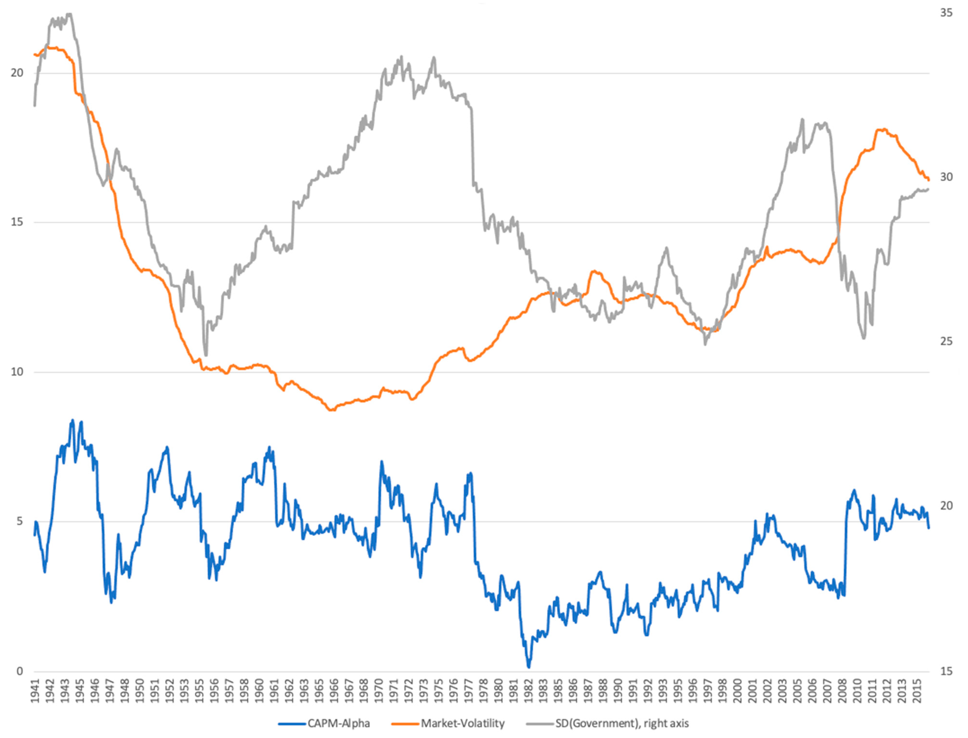
In the following, I analyze the time-series properties of the GOV2 strategy. In Figure 4, I show the rolling window CAPM alphas of the GOV2 strategy, market volatility, and the standard deviation of the policy-related uncertainty measure. The figure presents the annualized CAPM alpha of the dynamic trading strategy for rolling 15-year windows. Each point in the graph corresponds to using the previous 15 years of data. Apparently, the CAPM-alpha of our strategy is not necessarily different during subsamples when volatility is relatively high. The subsample CAPM-alpha typically fluctuates around 5%, except during the time period 1980–2000. This should not be surprising as our results rely on a large degree of variation in policy-related uncertainty about work. Variations in policy-related uncertainty were relatively low over this period; hence, my strategy is not very different from a buy-and-hold strategy and alphas are low.
The findings presented in Table 3 Panel A suggests that the ‘stock market-related-uncertainty-expected-return’ relationship, like the market volatility-expected return relationship, is on average, negative4. As discussed earlier, Moreira and Muir (2017) propose a related market volatility-based trading strategy that takes less risk when market volatility is high. Similarly, I analyze a stock market uncertainty-based trading strategy that takes less risk (decreases the weights) when stock market uncertainty is high. Hence, the scaled portfolio weight in the original market factor at time t+1 is given by , where SMU refers to my measure of stock market uncertainty. As a result, I invest more (less) when past uncertainties have been below (above) the target. Again, I choose a target that produces scaled portfolio returns with the same ex-post volatility compared to the (unscaled) market factor. When analyzing the ‘stock market-related-uncertainty-expected-return’ relationship in Table 3 Panel C, the results suggest that it is typically positive, but turns negative during recessions. Hence, in the following, I design a dynamic to take into account this particular feature of the data. I analyze a dynamic stock market uncertainty-based trading strategy that typically takes more risk when stock market uncertainty is high, but takes less risk when stock market uncertainty is high. Hence, the scaled portfolio weight in the original market factor at time t+1 is given by during ‘normal’ times, but changes to during recessions. As a result, during ‘normal’ times, I invest more (less) when past uncertainties have been above (below) the particular ‘normal target’ and during recessions, I invest more (less) when past uncertainties have been below (above) the particular ‘recession target’. Again, I choose targets that produce scaled portfolio returns with the same ex-post volatility compared to the (unscaled) market factor. While both trading strategies generate a significantly positive market risk-adjusted alpha, the dynamic stock market uncertainty-based trading strategy clearly outperforms the static one with a CAPM-alpha (p-value) of 4.6% (0.00) and 3% (0.04), respectively. Unsurprisingly, similar to the market-volatility-timing, both strategies do not ‘survive’ the further risk-adjustments. Hence, these results suggest that the positive risk-return still holds during ‘normal’ times, but becomes significantly weaker during crisis periods. Importantly, the market volatility-based trading strategy proposed Moreira and Muir (2017), which takes less risk when market volatility is high, seems to only pick up a feature of the data during crisis periods. In light of the controversies surrounding the divergent governmental policy approaches taken by Republicans and Democrats, I further examine the variations in the uncertainty-managed portfolio contingent on which political party holds the majority in the Senate. In general, I believe that, when Republicans hold a majority, there is less uncertainty around governmental policies. At the 1% level, the average government measure throughout these times is 0.75, and, during times when Democrats hold a majority in the Senate, it is 0.98. According to the earlier research, one may anticipate that the government plan would perform especially well at times when the Republicans hold a majority in the Senate because of the decreased level of uncertainty. In order to understand the magnitude of this effect, I run the following regression,
which gives the relative beta of the scaled factor conditional on the Republicans having the majority in senate () compared to the unconditional estimate. I find that the “Republicans market beta” is significantly lower compared to the “Democrats market beta”, which suggests that the government-managed strategy takes less risk during periods when the Republicans have the majority in senate. The Democrats market beta of the managed market factor is 1.05 (t-stat 19.46) while the Republicans market beta coefficient is −0.30 (t-stat −9.59), making the beta of the managed portfolio conditional on a Republicans period equal to 0.75. By taking more risk in a high policy-related uncertain market, the monthly CAPM alpha decreases to 0.23% during Democrats periods, from 0.33% during Republicans periods.
4. Conclusions
Forward-looking metrics of uncertainty, derived from options-implied data, are expected to be strong predictors of equity market returns, as per asset pricing theory. However, empirical studies find only a weak statistical relationship of the VIX, for example, with returns. Unlike studies that typically focus on short time series of option prices, I utilize a ‘VIX-type’ uncertainty measure based on textual analysis, which starts in 1890 and is constructed using the titles and abstracts of front-page articles from the Wall Street Journal. I hypothesize that uncertainty timing could enhance Sharpe ratios because fluctuations in uncertainty do not always correlate with changes in equity risk. As a result, these fluctuations may not be counterbalanced by proportional changes in expected returns. I find that, firstly, since market volatility has a strong and substantial predictive capacity for momentum profits, momentum is the driving force behind this unexpected feature in the data. Secondly, I demonstrate, using data from the US stock market, that future excess returns on the market portfolio at the short horizon can be explained by lagged news-based uncertainty. These predictability results are mostly driven by policy and war-related concerns, whereas news about the stock market has no predictive power. An annualized equity risk-adjusted alpha of 5.33% and an appraisal ratio of 0.46 are produced by a managed equity portfolio that assumes greater risk when news-based uncertainty is high. Thirdly, contrary to popular investment knowledge, managing news-based uncertainty involves comparatively lower risk during recessions. Because it excludes common risk-based explanations, this makes it difficult to construct models of time-varying expected returns. Fourthly, due to less ambiguity around government policy, and by assuming less risk, my trading strategy performs better during times when the Republicans control the senate.
Funding
This research received no external funding.
Data Availability Statement
Data were obtained from Asaf Manela and are available at http://apps.olin.wustl.edu/faculty/manela/data.html (accessed on 7 March 2023).
Conflicts of Interest
The author declares no conflict of interest.
| 1 | The results of Adrian et al. (2019) suggest that the relationship is nonlinear, which partly explains why VIX does not forecast stock returns significantly at any horizon. |
| 2 | It could be argued that news-based metrics depend on coverage of the weekend news that hasn’t been priced into the stock market yet. In order to address these issues, Manela and Moreira (2017) omit a month from the predictability regressions. |
| 3 | Alternatively, I choose a target that produces scaled portfolio returns with the same ex-post downside risk compared to the (unscaled) market factor, where downside risk is defined as the 1-month, 5% Value-at-Risk using the historical simulation approach. However, the results qualitatively do not change. |
| 4 | The correlation of the stock market uncertainty measure and market volatility is 45% in my sample. |
References
- Adrian, Tobias, Richard K. Crump, and Erik Vogt. 2019. Nonlinearity and Flight-to-Safety in the Risk-Return Trade-Off for Stocks and Bonds. The Journal of Finance 74: 1931–73. [Google Scholar] [CrossRef]
- Ai, Hengjie, Leyla Jianyu Han, and Lai Xu. 2022. Information-Driven Volatility. SSRN, 3961096. [Google Scholar] [CrossRef]
- Baker, Scott R., Nicholas Bloom, Steven J. Davis, and Kyle J. Kost. 2023. Policy News and Stock Market Volatility. Working Paper. Cambridge: National Bureau of Economic Research. [Google Scholar]
- Barroso, Pedro, and Pedro Santa-Clara. 2015. Momentum has its moments. Journal of Financial Economics 116: 111–20. [Google Scholar] [CrossRef]
- Bollerslev, Tim, and Viktor Todorov. 2011. Tails, fears, and risk premia. Journal of Finance 66: 2165–211. [Google Scholar] [CrossRef]
- Bollerslev, Tim, George Tauchen, and Hao Zhou. 2009. Expected stock returns and variance risk premia. Review of Financial Studies 22: 4463–92. [Google Scholar] [CrossRef]
- Drechsler, Itamar. 2013. Uncertainty, time-varying fear, and asset prices. The Journal of Finance 68: 1843–89. [Google Scholar] [CrossRef]
- Drechsler, Itamar, and Amir Yaron. 2011. What’s vol got to do with it. Review of Financial Studies 24: 1–45. [Google Scholar] [CrossRef]
- Frazzini, Andrea, and Lasse Heje Pedersen. 2014. Betting Against Beta. Journal of Financial Economics 111: 1–25. [Google Scholar] [CrossRef]
- Gabaix, Xavier. 2012. Variable rare disasters: An exactly solved framework for ten puzzles in macro-finance. Quarterly Journal of Economics 127: 645–700. [Google Scholar] [CrossRef]
- Gourio, Francois. 2012. Disaster risk and business cycles. American Economic Review 102: 2734–66. [Google Scholar] [CrossRef]
- Koenker, Roger, and Quanshui Zhao. 1994. L-estimation for linear heteroscedastic models. Journal of Nonparametric Statistics 3: 223–235. [Google Scholar] [CrossRef]
- Lehnert, Thorsten. 2023. Environmental Policy and Equity Prices. PLoS ONE 18: e0289397. [Google Scholar] [CrossRef] [PubMed]
- Manela, Asaf, and Alan Moreira. 2017. News implied volatility and disaster concerns. Journal of Financial Economics 123: 137–62. [Google Scholar] [CrossRef]
- Merton, Robert C. 1973. An intertemporal capital asset pricing model. Econometrica 41: 867–87. [Google Scholar] [CrossRef]
- Moreira, Alan, and Tyler Muir. 2017. Volatility-managed portfolios. Journal of Finance 72: 1611–44. [Google Scholar] [CrossRef]
- Murphy, Kevin M., and Robert H. Topel. 2002. Estimation and inference in two-step econometric models. Journal of Business and Economic Statistics 20: 88–97. [Google Scholar] [CrossRef]
- Newey, Whitney K., and Kenneth D. West. 1987. A simple, positive semi-definite, heteroskedasticity and autocorrelation consistent covariance matrix. Econometrica 55: 703–8. [Google Scholar] [CrossRef]
- Novy-Marx, Robert, and Mihail Velikov. 2021. Forthcoming. Betting Against Betting Against Beta. Journal of Financial Economics 143: 80–106. [Google Scholar] [CrossRef]
- Wachter, Jessica A. 2013. Can time-varying risk of rare disasters explain aggregate stock market volatility? Journal of Finance 68: 987–1035. [Google Scholar] [CrossRef]
- Wang, Kevin Q., and Jianguo Xu. 2015. Market volatility and momentum. Journal of Empirical Finance 30: 79–91. [Google Scholar] [CrossRef]
Figure 1.
Charts on the previous month’s policy-related uncertainty. In Figure 1, I categorize the returns for the subsequent month into five buckets using the monthly time-series of lagged policy-related uncertainty. The lowest, “LOW GOV”, examines the characteristics of returns for the month that follows the months with the lowest 20% of policy-related uncertainty. In the following month, I display the average return, the standard deviation, and the average return divided by variance.
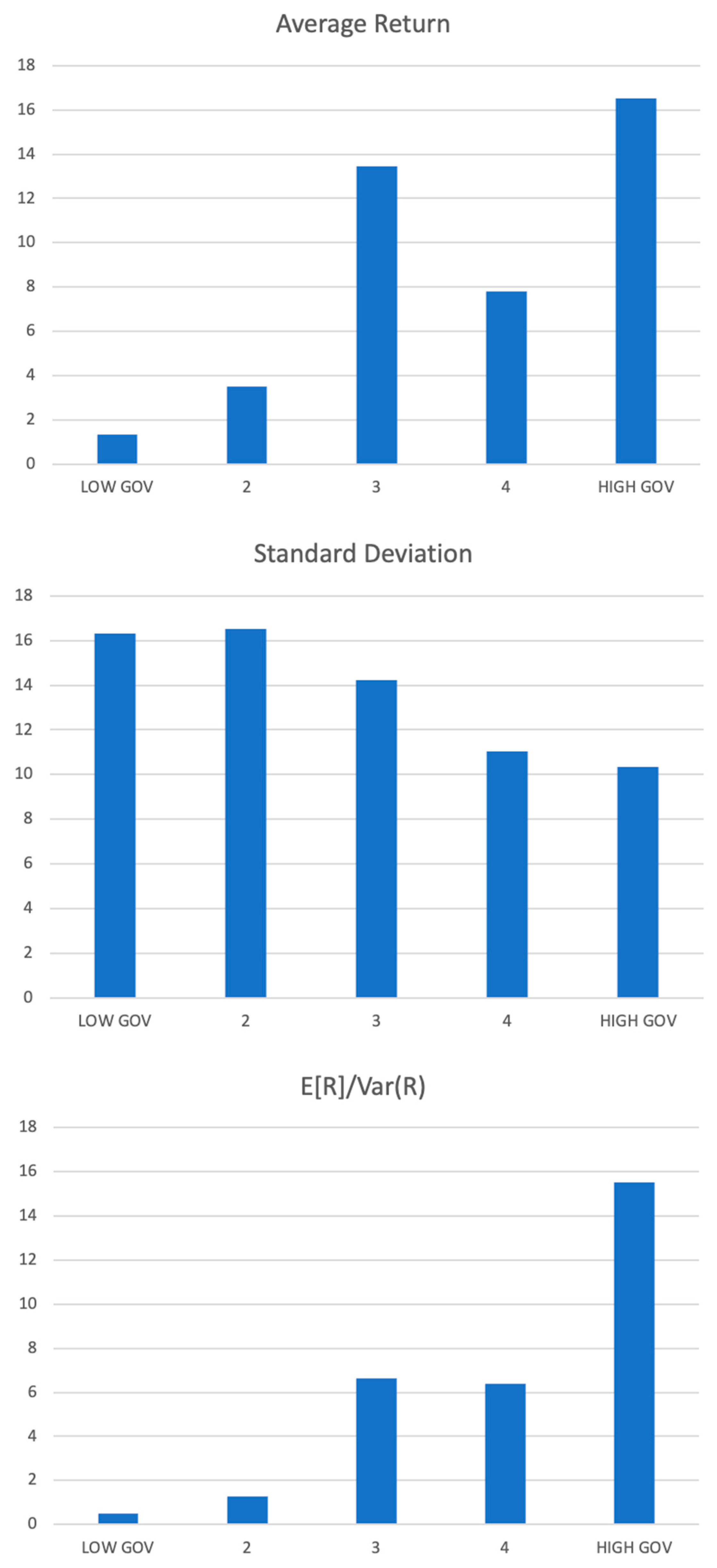
Figure 2.
Performance of the volatility-managed trading strategy. The figure presents the cumulative returns of the passive strategy (the market portfolio) and the two dynamic trading strategies (volatility- and variance-managing the market portfolio) based on $100 invested in August 1926. For better comparison, on the y-axis, a logarithmic scale is used to display the numerical data that span a broad range of values. The red bars represent the NBER recession periods.
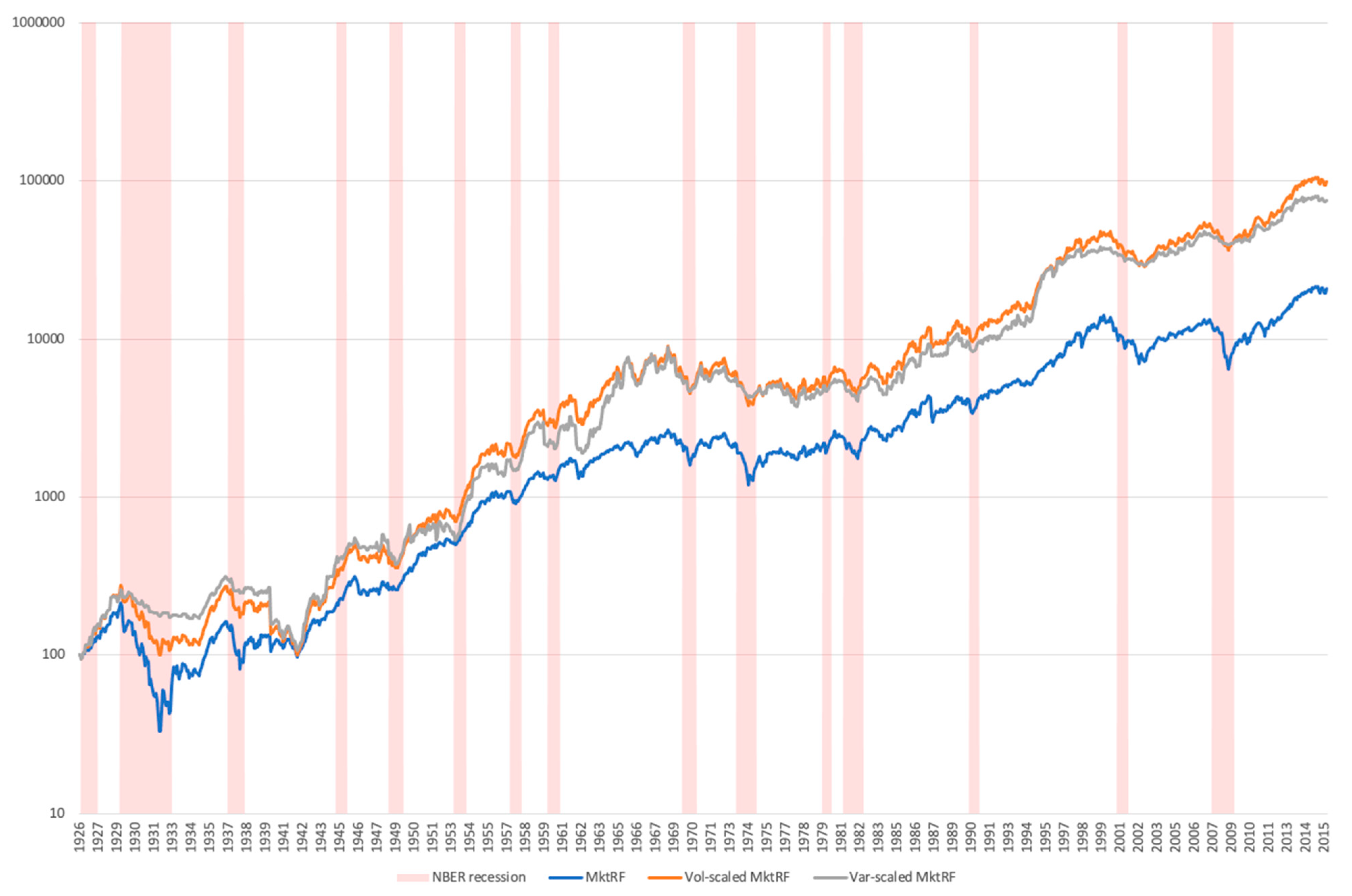
Figure 3.
Performance of the policy uncertainty (GOV)-managed trading strategy. The figure presents the cumulative returns of the passive strategy (the market portfolio) and the two dynamic trading strategies (GOV- and GOV2-managing the market portfolio) based on $100 invested in August 1926. For better comparison, on the y-axis, a logarithmic scale is used to display the numerical data that span a broad range of values. The red bars represent the NBER recession periods.
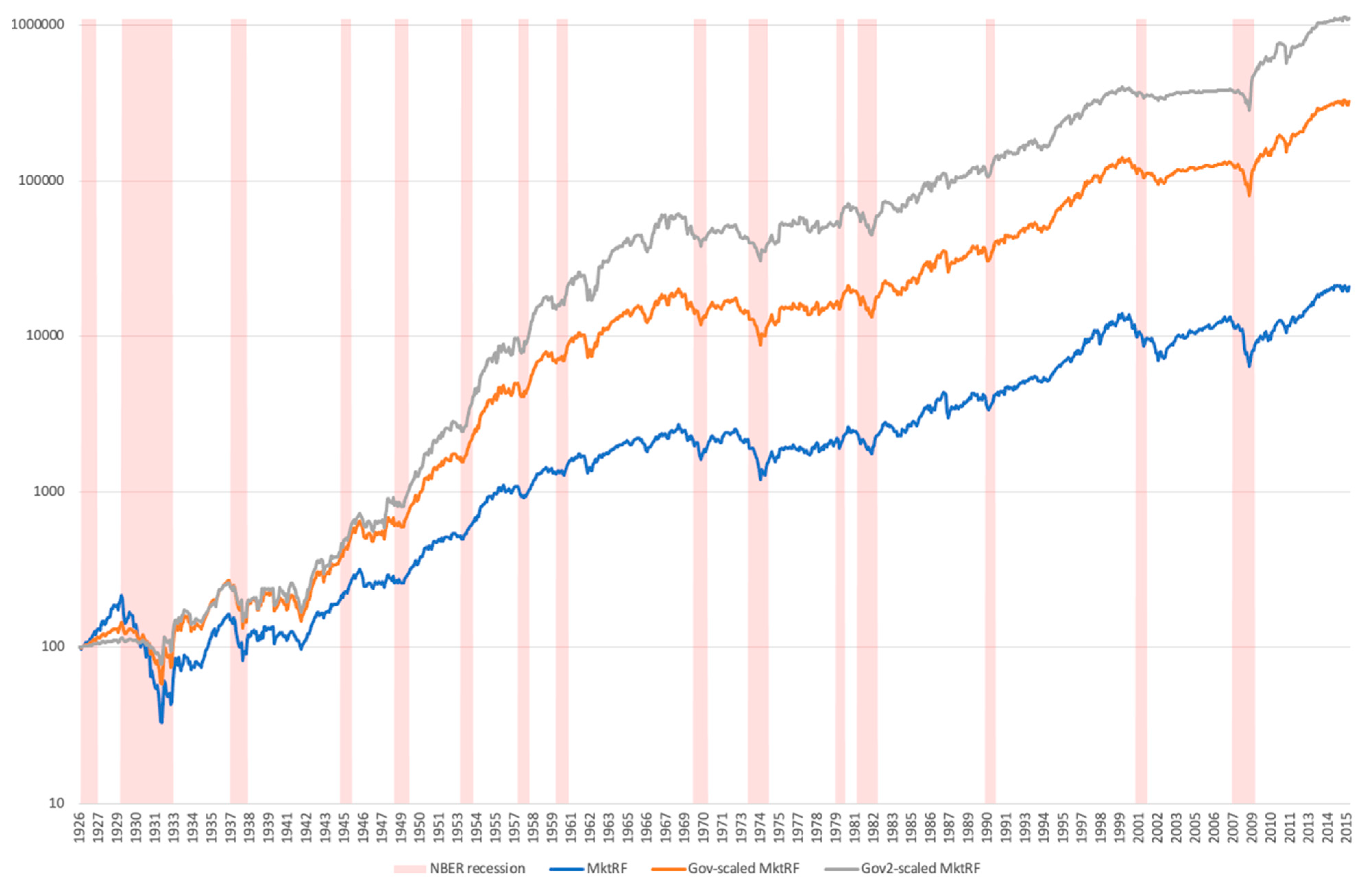
Figure 4.
Rolling Window CAPM Alpha. The figure presents the annualized CAPM alpha of the dynamic trading strategy (the GOV2-managed portfolio) for rolling 15-year windows. Each point in the graph corresponds to the previous 15 years of data. I also plot the average experienced market volatility and the standard deviation of the policy-related uncertainty (Government) for the same window of the previous 15 years.

Table 1.
Summary Statistics. The market excess return, other factor portfolio returns, option-implied volatility, and news-implied uncertainty measures employed in the study are all summarized in the table. The entire sample period, which spans 1077 months, runs from July 1926 to March 2016. The excess market return, or MktRF, is the value-weighted returns of NYSE, Amex, and Nasdaq stocks over the 30-day T-bill return expressed as a percentage by the Centre for Research in Security Prices (CRSP). SMB (Small Minus Big) and HML (High Minus Low) are historic excess returns of small-cap companies over large-cap companies and historic excess returns of value stocks (which have a high book-to-price ratio) over growth stocks (which have a low book-to-price ratio), respectively. A momentum factor (MOM) and both legs of the MOM factor (Winner and Loser) are also included. The Novy-Marx and Velikov (2021) version of the original betting-against-beta factor (EWBAB) and their modified version (VWBAB), which was built using more standard processes, are additional factors. The CBOE’s risk-neutral volatility indexes are VIX and VXO. NVIX is a text-based measure of uncertainty that uses the titles and abstracts of front-page articles of the Wall Street Journal. It consists of six word categories related to Government, Intermediation, Natural Disasters, Stock Markets, and War. The orthogonal component of NVIX that is not explained by the five interpretable word categories is unclassified.
| Mean | Median | Std. | Min | Max | |
|---|---|---|---|---|---|
| MktRF | 0.65 | 1.01 | 5.39 | −29.13 | 38.85 |
| SMB | 0.19 | 0.10 | 3.18 | −17.29 | 36.56 |
| HML | 0.36 | 0.14 | 3.49 | −13.11 | 36.61 |
| MOM (1927:01–2016:03) | 0.65 | 0.81 | 4.71 | −52.05 | 18.20 |
| Winner (1927:01–2016:03) | 1.40 | 1.89 | 6.13 | −27.92 | 43.93 |
| Loser (1927:01–2016:03) | 0.75 | 0.67 | 8.10 | −38.06 | 84.34 |
| EWBAB (1931:02–2016:03) | 0.78 | 0.87 | 3.20 | −23.44 | 16.23 |
| VWBAB (1931:02–2016:03) | 0.40 | 0.52 | 3.65 | −27.28 | 16.41 |
| VIX (1990:01–2016:03) | 19.88 | 18.24 | 7.55 | 10.42 | 59.89 |
| VXO (1986:06–2016:03) | 20.70 | 18.74 | 8.34 | 9.54 | 61.41 |
| NVIX | 24.70 | 24.46 | 4.64 | 13.62 | 57.90 |
| Government | 0.90 | 0.88 | 0.36 | 0.20 | 2.21 |
| Intermediation | 0.51 | 0.36 | 0.71 | −0.73 | 6.67 |
| NaturalDisaster | −0.16 | −0.01 | 0.03 | −0.29 | 0.03 |
| StockMarket | 2.04 | 1.57 | 0.77 | 0.10 | 12.04 |
| War | 0.28 | 0.13 | 0.57 | −0.25 | 3.93 |
| Unclassified | 8.23 | 8.14 | 3.48 | −1.59 | 35.96 |
Table 2.
Risk Premia. The table presents the coefficients from the monthly return predictability regressions based on news implied volatility (NVIX). The full sample period ranges from July 1926 to March 2016, covering a total of 1077 months. The dependent variable, MktRF, is the excess market return, the value-weighted returns of NYSE, Amex, and Nasdaq stocks from the Center for Research in Security Prices (CRSP) over 30-day T-bill return in %. NVIX is a text-based measure of uncertainty that uses the titles and abstracts of front-page articles of the Wall Street Journal. VXO is the CBOE risk-neutral volatility index. Explanatory variables are normalized to have unit standard deviation over the entire sample. In Panel A and B, are p-values based on Newey and West (1987) standard errors with the same number of lags as the forecasting window. are p-values based on (wild) bootstrapped standard errors that further account for the fact that the regressor is estimated in a first stage. In Panel C and D, p-values are based on robust standard errors, which are computed according to the sandwich estimator developed in Koenker and Zhao (1994). AIC is the Akaike information criterion, where the preferred model is the one with the minimum AIC value. **, and *** indicate 5%, and 1% significance levels, respectively.
| Panel A: Full Sample | Panel B: 1986–2016 | ||||
| NVIX | NVIX | VXO | |||
| 0.24 | 0.30 | 0.49 | |||
| [0.17] | [0.15] | [0.17] | |||
| [0.21] | [0.18] | ||||
| 0.11% | 0.51% | 0.43% | |||
| Panel C: Full Sample | Panel D: 1986–2016 | ||||
| NVIX | NVIX | VXO | |||
| 0.25 | −0.08 | −0.00 | −0.33 | ||
| [0.67] | [0.58] | [0.76] | |||
| 0.50 | 0.34 ** | 0.25 | 0.49 | ||
| [0.02] | [0.14] | [0.12] | |||
| 0.75 | 0.68 *** | 0.81 *** | 0.95 *** | ||
| [0.00] | [0.00] | [0.00] | |||
| AIC | 6494 | 2078 | 2080 | ||
Table 3.
Risk Premia: Word Categories. The table presents the coefficients from the monthly return predictability regressions based on word categories constructed from news implied volatility (NVIX). The full sample period ranges from July 1926 to March 2016, covering a total of 1077 months. The dependent variable, MktRF, is the excess market return, the value-weighted returns of NYSE, Amex, and Nasdaq stocks from the Center for Research in Security Prices (CRSP) over 30-day T-bill return in %. NVIX is a text-based measure of uncertainty that uses the titles and abstracts of front-page articles of the Wall Street Journal. It consists of six word categories (and the corresponding measure ) related to Government, Intermediation, Natural Disasters, Stock Markets, and War. Unclassified is the orthogonal component of NVIX that is not explained by the five interpretable word categories. is a regression dummy, which is set at 1 during NBER recession months. Explanatory variables are normalized to have unit standard deviation over the entire sample. In Panel A and C, are p-values based on Newey and West (1987) standard errors with the same number of lags as the forecasting window. are p-values based on (wild) bootstrapped standard errors that further account for the fact that the regressor is estimated in a first stage. In Panel B, p-values are based on robust standard errors, which are computed according to the sandwich estimator developed in Koenker and Zhao (1994). AIC is the Akaike information criterion, where the preferred model is the one with the minimum AIC value. *, **, and *** indicate 10%, 5%, and 1% significance levels, respectively.
| Panel A: | |||||||
| Government | Intermediation | NaturalDisaster | StockMarket | War | Unclassified | ||
| 0.52 *** | 0.21 | 0.04 | −0.08 | 0.32 *** | 0.06 | ||
| [0.00] | [0.29] | [0.75] | [0.72] | [0.00] | [0.18] | ||
| [0.00] | [0.30] | [0.75] | [0.72] | [0.01] | [0.19] | ||
| 0.85% | 0.06% | 0.00% | 0.00% | 0.42% | 0.07% | ||
| Panel B: | |||||||
| Government | Intermediation | NaturalDisaster | StockMarket | War | Unclassified | ||
| 0.25 | 0.64 *** | −0.19 | −0.11 | −0.73 ** | 0.46 ** | −0.04 | |
| [0.00] | [0.50] | [0.62] | [0.02] | [0.04] | [0.86] | ||
| 0.50 | 0.37 *** | 0.34 * | 0.12 | 0.06 | 0.21 ** | 0.23 | |
| [0.01] | [0.06] | [0.25] | [0.76] | [0.02] | [0.16] | ||
| 0.75 | 0.10 * | 0.49 ** | 0.40 *** | 0.58 *** | 0.33 * | 0.59 *** | |
| [0.08] | [0.02] | [0.00] | [0.00] | [0.08] | [0.00] | ||
| 6492 | 6495 | 6501 | 6502 | 6496 | 6496 | ||
| Panel C: | |||||||
| Government | Intermediation | NaturalDisaster | StockMarket | War | Unclassified | ||
| 0.15 | 0.31 | 0.19 | 0.45 ** | 0.20 * | 0.37 ** | ||
| [0.30] | [0.11] | [0.18] | [0.03] | [0.03] | [0.02] | ||
| [0.35] | [0.12] | [0.19] | [0.04] | [0.10] | [0.02] | ||
| 1.45 *** | −0.11 | −0.65 | −0.75 * | 0.65 ** | −0.16 | ||
| [0.00] | [0.80] | [0.17] | [0.09] | [0.03] | [0.72] | ||
| [0.00] | [0.84] | [0.18] | [0.10] | [0.04] | [0.80] | ||
| 2.99% | 1.19% | 1.15% | 1.43% | 1.50% | 1.32% | ||
Table 4.
Risk adjustment for MktRF-based strategies. The alphas and factor loadings from the time-series regressions of the dynamic trading strategies’ monthly returns on equity risk factors are shown in the table. The entire sample period, which spans 1077 months, runs from July 1926 to March 2016. The excess market return, or MktRF, is the value-weighted returns of NYSE, Amex, and Nasdaq stocks over the 30-day T-bill return expressed as a percentage by the Centre for Research in Security Prices (CRSP). Additional factors include the Novy-Marx and Velikov (2021) version of the original betting-against-beta factor (EWBAB) and their updated version (VWBAB), which was built using more standardized processes, as well as the size (SMB), value (HML), and momentum (MOM). The coefficient estimates for each regression are shown in the first row, and the heteroskedasticity-adjusted p-values (in parenthesis) are reported in the second row. ***, ** and * indicate statistical significance at the 1%, 5% and 10% level, respectively.
| Panel A: Volatility-Managed Market Factor | ||||||||
| a (%) | Mkt-Rf | SMB | HML | MOM | EWBAB | VWBAB | Adj. R2 | |
| Vol-Scaled MktRf | 0.30 *** | 0.88 *** | −0.02 | −0.18 *** | 0.74 | |||
| (0.00) | (0.00) | (0.72) | (0.00) | |||||
| 0.11 | 0.92 *** | −0.01 | −0.09 ** | 0.19 *** | 0.76 | |||
| (0.22) | (0.00) | (0.84) | (0.05) | (0.00) | ||||
| 0.07 | 0.92 *** | −0.01 | −0.11 ** | 0.18 *** | 0.04 | 0.75 | ||
| (0.51) | (0.00) | (0.93) | (0.02) | (0.00) | (0.38) | |||
| 0.04 | 0.94 *** | 0.02 | −0.11 ** | 0.17 *** | 0.11 *** | 0.77 | ||
| (0.22) | (0.00) | (0.78) | (0.01) | (0.00) | (0.00) | |||
| Var-Scaled MktRf | 0.41 *** | 0.66 | −0.05 | −0.17 ** | 0.41 | |||
| (0.00) | (0.00) | (0.38) | (0.01) | |||||
| 0.16 | 0.72 | −0.04 | −0.05 | 0.25 *** | 0.44 | |||
| (0.22) | (0.00) | (0.51) | (0.29) | (0.00) | ||||
| 0.11 | 0.72 | −0.03 | −0.07 | 0.23 *** | 0.04 | 0.44 | ||
| (0.54) | (0.00) | (0.59) | (0.14) | (0.00) | (0.50) | |||
| 0.09 | 0.74 | −0.01 | −0.08 | 0.22 *** | 0.11 ** | 0.45 | ||
| (0.54) | (0.00) | (0.86) | (0.11) | (0.00) | (0.02) | |||
| Panel B: Uncertainty-Managed Market Factor | ||||||||
| a (%) | Mkt-Rf | SMB | HML | MOM | EWBAB | VWBAB | Adj. R2 | |
| Gov-scaled MktRf | 0.25 *** | 0.94 *** | 0.02 | 0.01 | 0.04 * | 0.87 | ||
| (0.00) | (0.00) | (0.28) | (0.32) | (0.09) | ||||
| 0.25 *** | 0.94 *** | 0.01 | 0.01 | 0.05 * | 0.01 | 0.88 | ||
| (0.00) | (0.00) | (0.62) | (0.75) | (0.09) | (0.89) | |||
| 0.24 *** | 0.94 *** | 0.02 | 0.01 | 0.04 * | 0.02 | 0.88 | ||
| (0.00) | (0.00) | (0.48) | (0.81) | (0.09) | (0.93) | |||
| Gov2-scaled MktRf | 0.44 *** | 0.79 *** | 0.03 | 0.02 | 0.07 | 0.61 | ||
| (0.00) | (0.00) | (0.51) | (0.59) | (0.18) | ||||
| 0.44 *** | 0.85 *** | 0.01 | 0.01 | 0.07 | 0.00 | 0.64 | ||
| (0.00) | (0.00) | (0.86) | (0.96) | (0.15) | (0.87) | |||
| 0.43 *** | 0.85 *** | 0.01 | −0.01 | 0.07 | 0.04 | 0.64 | ||
| (0.00) | (0.00) | (0.72) | (0.96) | (0.18) | (0.39) | |||
Disclaimer/Publisher’s Note: The statements, opinions and data contained in all publications are solely those of the individual author(s) and contributor(s) and not of MDPI and/or the editor(s). MDPI and/or the editor(s) disclaim responsibility for any injury to people or property resulting from any ideas, methods, instructions or products referred to in the content. |
© 2025 by the author. Licensee MDPI, Basel, Switzerland. This article is an open access article distributed under the terms and conditions of the Creative Commons Attribution (CC BY) license (https://creativecommons.org/licenses/by/4.0/).
Share and Cite
MDPI and ACS Style
Lehnert, T. Political Uncertainty-Managed Portfolios. Risks 2025, 13, 55. https://doi.org/10.3390/risks13030055
AMA Style
Lehnert T. Political Uncertainty-Managed Portfolios. Risks. 2025; 13(3):55. https://doi.org/10.3390/risks13030055
Chicago/Turabian StyleLehnert, Thorsten. 2025. "Political Uncertainty-Managed Portfolios" Risks 13, no. 3: 55. https://doi.org/10.3390/risks13030055
APA StyleLehnert, T. (2025). Political Uncertainty-Managed Portfolios. Risks, 13(3), 55. https://doi.org/10.3390/risks13030055
Note that from the first issue of 2016, this journal uses article numbers instead of page numbers. See further details here.