On the Curvature of the Bachelier Implied Volatility

Abstract

Our aim in this paper is to analytically compute the at-the-money second derivative of the Bachelier implied volatility curve as a function of the strike price for correlated stochastic volatility models. We also obtain an expression for the short-term limit of this second derivative in terms of the first and second Malliavin derivatives of the volatility process and the correlation parameter. Our analysis does not need the volatility to be Markovian and can be applied to the case of fractional volatility models, both with $H<1/2$ and $H>1/2.$ More precisely, we start our analysis with an adequate decomposition formula of the curvature as the curvature in the uncorrelated case (where the Brownian motions describing asset price and volatility dynamics are uncorrelated) plus a term due to the correlation. Then, we compute the curvature in the uncorrelated case via Malliavin calculus. Finally, we add the corresponding correlation correction and we take limits as the time to maturity tends to zero. The presented results can be an interesting tool in financial modeling and in the computation of the corresponding Greeks. Moreover, they allow us to obtain general formulas that can be applied to a wide class of models. Finally, they provide us with a precise interpretation of the impact of the Hurst parameter H on this curvature.

1. Introduction

Classical models in option pricing are strongly based on the Black–Scholes model, where asset prices are described as a geometric Brownian motion (and then market prices are positive) that depends on interest rates and the volatility of the market. More precisely, in a Black–Scholes model, asset prices $S_t$ are assumed to follow a stochastic differential equation of the form

$$d{S}_t=r{S}_{t}dt+\sigma S_{t}d{W}_t,$$

where r and $\sigma$ are two constants that denote the interest rate and the volatility of the market, respectively. Some classical references include Gatheral (2006), Hagan et al. (2002) and Mendevev and Scaillet (2007).

The risk of negative prices has been historically neglected. Nevertheless, in recent years (particularly in sectors such as interest rates, commodities, and energy markets), negative prices represent a new risk that has gained attention. For example, after the crisis in 2008 when the interest rate turned negative and the log-normal implied volatility market exploded when the screens of the main market contributors showed that floors with a strike of zero had a positive value, there was a transition from the Black–Scholes model to the shifted Black–Scholes model, and from the shifted Black–Scholes model to the Bachelier model. Another scenario in which the Bachelier model played a special role was during the COVID-19 crisis and the collapse of future oil prices, which reached negative price levels.

In this context, the Bachelier model (see Bachelier (1900)), which assumes a normal distribution for asset prices, has attracted attention due to its ability to handle negative price levels. This ability to model negative prices has significant implications for risk managers and financial institutions. The Bachelier model enables more accurate estimates of tail risk and potential extreme events that could lead to negative asset values. Nevertheless, the Bachelier model is not able to reproduce the complexity of real market data. Thus, as in Black–Scholes-based models, some extensions have to be considered. Among them, the most common modification is to allow the volatility process to be a stochastic process. And in the study of these models, one of the key concepts is the study of the Bachelier implied volatility and its main differences when compared with the classical Black-Scholes implied volatility. The computation of prices and implied volatilities under this model has been presented in, for example, Terakado (2019). In a recent paper (see Alos et al. (2023)), the at-the-money short-end level and skew were computed using techniques of Malliavin calculus. The results proved that the short-end behaviour of the Bachelier implied volatility is highly dependent (as the Black–Scholes implied volatility) on the roughness of the volatility process.

In this paper, we focus on the study of the at-the-money Bachelier implied curvature, following similar ideas to those expressed by in Alòs and Leòn (2017). Knowing the curvature in the short term is highly important for practitioners. The main reason is that the curvature provides a way to determine whether the dynamics of the volatility smile in the short term are correctly captured by the model used for portfolio management. Moreover, having a closed-form expression for the short-term curvature allows for the calculation of second-order Greeks, which tend to be quite unstable when the expiration date is close to the valuation date. Our approach, based on Malliavin calculus, is very general and becomes a tool to study this curvature for a wide class of models and scenarios.

The paper is organized as follows. A revision of the literature is provided in Section 2. In Section 3, we present the problem and notations. Section 4 gives an introduction to the main concepts on Malliavin calculus used in our analysis. Section 5 is devoted to introducing some previous results on Bachelier prices and implied volatilities. The uncorrelated case (where the Brownian motions driving asset prices and volatilities are independent) is studied in Section 6. The correlated case and the main results are discussed in Section 7. Finally, some examples are presented in Section 8.

2. Revision of the Literature

The Bachelier model was introduced in Bachelier (1900) as a first attempt to describe random asset prices. In modern finance, it has been addressed in the context of interest rates and commodities, as for example in Hagan et al. (2002). A comparison between the Bachelier and the Black–Scholes models is studied in Schachermayer and Teichmann (2008). In recent years, some literature on practical issues is emerging, as for example in Terakado (2019).

3. Statement of the Problem and Notation

In this paper, we consider the following Bachelier-type model for the price of a stock under a risk-neutral probability measure P:

$$S_t=S_0+{\int }_0^t{\sigma }_s\left(\rho d{W}_s+\sqrt{1-{\rho }^2}d{B}_s\right),t\in [0,T].$$

(1)

Here, W and B are standard Brownian motions defined on a complete probability space $(\mathsf{\Omega },\mathcal{G},P)$, and $\sigma$ is a square-integrable and right-continuous stochastic process adapted to the filtration generated by W. In the following, ${\mathcal{F}}^W$ and ${\mathcal{F}}^B$ denote the filtrations generated by W and B. Moreover we define $\mathcal{F}:={\mathcal{F}}^W\vee {\mathcal{F}}^B.$ Notice that we assume the interest rate r to be zero. This is not a lack of generality, since r is assumed to be zero in interest rate models, while the underlying asset in commodity derivatives is future prices. In the case where $\sigma$ is constant and $\rho =0$, the above model is called the Bachelier model.

It is well known that there is no arbitrage opportunity if we price an European call with strike price K using the formula

$$V_t=E_t\left[{(S_T-K)}_{+}\right],$$

where $E_t$ is the ${\mathcal{F}}_t$-conditional expectation with respect to P (i.e., $E_t\left(Z\right)=E\left(Z\right|{\mathcal{F}}_t)$). Following this, we make use of the following notation:

• $v_t^2={\displaystyle \frac{1}{T-t}}{\int }_t^T{\sigma }_u^{2}du.$ That is, v represents the future average volatility.
• $M_t=E_t\left({\int }_0^T{\sigma }_u^{2}du\right),t\in \left[0,T\right]$.
• $Bac(t,x,k,\sigma )$ denotes the price of an European call option under the classical Bachelier model with constant volatility $\sigma$, current stock price x, time to maturity $T-t,$ strike price k, and interest rate $r=0$. That is,

  $$Bac(t,x,k,\sigma )=(x-k)N\left(d_{Bac}(k,\sigma )\right)+N^{\prime }\left(d_{Bac}(k,\sigma )\right)\sigma \sqrt{T-t},$$

  with

  $$d_{Bac}(k,\sigma )={\displaystyle \frac{x-k}{\sigma \sqrt{T-t}}},$$

  where N is the cumulative distribution function and the probability density function of the standard normal random variable.
  ${\mathcal{L}}_{Bac}\left(\sigma \right)$ denotes the Bachelier differential operator with volatility $\sigma :$

  $${\mathcal{L}}_{Bac}\left(\sigma \right)={\displaystyle \frac{\partial }{\partial t}}+{\displaystyle \frac{1}{2}}{\sigma }^2{\displaystyle \frac{{\partial }^2}{\partial x^2}}$$
  It is well known that ${\mathcal{L}}_{Bac}\left(\sigma \right)Bac\left(·,·,·;\sigma \right)=0.$
• The Bachelier implied volatility $I_t^{Bac}\left(k\right)$ of a call option with strike k and market price $V_t$ is the unique volatility parameter one should put in the Bachelier formula to obtain the price $V_t$. That is, the quantity $I_t^{Bac}\left(k\right)$, such that

  $$V_t=Bac(t,S_t,k,I_t^{Bac}\left(k\right)),$$

  where $S_t$ denotes the asset price. Note that if $k=S_t$,

  $$V_t=Bac(t,S_t,S_t,I_t^{Bac}\left(S_t\right))=N^{\prime }\left(0\right)I_t^{Bac}\sqrt{T-t}={\displaystyle \frac{1}{\sqrt{2\pi }}}{I}_t^{Bac}\left(S_t\right)\sqrt{T-t}.$$

  (2)
  At the same time, due to the definition of the Black–Scholes implied volatility,

  $$V_t=Bac(t,S_t,S_t,I^{Bac}\left(S_t\right))=S_t\left(2N\left({\displaystyle \frac{I^{Bac}\left(S_t\right)\sqrt{T-t}}{2}}\right)-1\right).$$

  (3)
  Then, (2) and (3) imply the following conversion formula for ATM implied volatilities:

  $$I_t^{Bac}\left(S_t\right)={\displaystyle \frac{\sqrt{2\pi }}{\sqrt{T-t}}}{S}_t\left(2N\left({\displaystyle \frac{I^{Bac}\left(S_t\right)\sqrt{T-t}}{2}}\right)-1\right)$$

  (4)
  (see Choi (2022)). Further results on the difference between the Black–Scholes and the Bachelier implied volatilities can be found in Schachermayer and Teichmann (2008).

We will use the following notation for the Bachelier Gamma

$$G_{Bac}\left(t,x,k,\sigma \right):={\partial }_{xx}Bac\left(t,x,k,\sigma \right)$$

Notice that the following Gamma–Vega relationship holds

$$G_{Bac}={\displaystyle \frac{1}{T\sigma }}{\partial }_{\sigma }Bac$$

In order to prove our results on the implied volatility smile, we make use of the following results on correlated stochastic volatility models (see Alos et al. (2023)).

Lemma 1. 

Let $0\le t\le s<T$, $\rho \in \left(-1,1\right)$ and ${\mathcal{G}}_t:={\mathcal{F}}_t\vee {\mathcal{F}}_T^W.$ Then, for every $n\ge 0,$ there exists $C=C(n,\rho )$, such that

$$\left|E\left(\left.{\partial }_x^n{G}_{Bac}\left(s,X_s,k,v_s\right)\right|{\mathcal{G}}_t\right)\right|\le C{\left({\int }_t^T{\sigma }_s^{2}ds\right)}^{-{\displaystyle \frac{1}{2}}\left(n+1\right)}.$$

4. Basic Concepts of Malliavin Calculus

In this section, we recall the key tools of Malliavin calculus that we use in this paper. We refer the reader to Alòs and García-Lorite (2023) for a deeper introduction to this topic and its applications in finance.

Basic Definitions

If $Z={\left(Z_t\right)}_{t\in [0,T]}$ is a standard Brownian motion, $\mathcal{S}$ denotes the set of random variables of the form

$$F=f(Z\left(h_1\right),\dots ,Z\left(h_n\right)),$$

(5)

where $h_1,\dots ,h_n\in L^2\left([0,T]\right)$, $Z\left(h_i\right)$ denotes the Wiener integral of $h_i$, for $i=1,\dots ,n$, and $f\in C_b^{\infty }\left({\mathbb{R}}^n\right)$ (i.e., f and all its partial derivatives are bounded). If $F\in \mathcal{S}$, the Malliavin derivative of F with respect to Z, $D^{Z}F$, is defined as the stochastic process in $L^2(\mathsf{\Omega }\times [0,T])$, given by

$$D_s^{Z}F=\sum _{j=1}^n{\displaystyle \frac{\partial f}{\partial x_j}}(W(h_1),\dots ,W(h_n))\left(s\right)h_j\left(s\right).$$

Moreover, for $m\ge 1$, we can define the iterated Malliavin derivative operator, $D^{m,Z}$, as

$$D_{s_1,\dots ,s_m}^{m,Z}F=D_{s_1}^Z\dots D_{s_m}^{Z}F,s_1,\dots ,s_m\in [0,T].$$

The operators $D^{m,Z}$ are closable in $L^2\left(\mathsf{\Omega }\right)$ and we denote by ${\mathbb{D}}_Z^{n,2}$ the closure of $\mathcal{S}$ with respect to the norm

$${\left|\right|F\left|\right|}_{n,2}={\left(E{\left|F\right|}^p+\sum _{i=1}^{n}E\left|\right|D^{i,Z}F{\left|\right|}_{L^2\left({[0,T]}^i\right)}^2\right)}^{{\displaystyle \frac{1}{2}}}.$$

Notice that the Malliavin derivative operator satisfies the chain rule. That is, given $f\in {\mathcal{C}}_Z^{1,2}$, and $F\in {\mathbb{D}}_Z^{1,2}$, the random variable $f\left(F\right)$ belongs to ${\mathbb{D}}_Z^{1,2}$, and $D^{Z}f\left(F\right)=f^{\prime }\left(F\right)D^{W}F$. We will also make use of the notation ${\mathbb{L}}^{n,2}={\mathbb{D}}_Z^{n,p}\left(L^2\left([0,T]\right)\right).$

Example 1. 

Consider a Black–Scholes model of the form $S_t=S_{0}exp(-{\displaystyle \frac{{\sigma }^2}{2}}+\sigma W_t)$, where S denotes asset prices, σ is the volatility parameter, and W is a Brownian motion. Then, the Malliavin derivative of $S_t$ with respect to W is given by

$$D_r^W{S}_t=\sigma S_t,$$

for $r<t$, and $D_r^W{S}_t=0$ for $r>t$.

Example 2. 

Consider now a process S of the form $S_t=S_{0}exp(-{\displaystyle \frac{{\sigma }^2}{2}}+\sigma W_t)$, where σ is a constant and $W^H$ is a Riemann–Liouville fractional Brownian motion of the form

$$W_t^H={\int }_0^t{(t-s)}^{H-{\displaystyle \frac{1}{2}}}d{W}_s,$$

for a certain Brownian motion W and a certain Hurst parameter H (see, for example, Alòs and García-Lorite (2023) for details). Then, the Malliavin derivative of $S_t$ with respect to W is given by

$$D_r^W{S}_t=\sigma {(t-r)}^{H-{\displaystyle \frac{1}{2}}}{S}_t,$$

for $r<t$, and $D_r^W{S}_t=0$ for $r>t$.

The adjoint of the derivative operator $D^Z$ is the divergence operator ${\delta }^Z$, which coincides with the Skorohod integral. Its domain, denoted by Dom $\delta$, is the set of processes $u\in L^2(\mathsf{\Omega }\times [0,T])$, such that there exists a random variable ${\delta }^Z\left(u\right)\in L^2\left(\mathsf{\Omega }\right)$, such that

$$E\left({\delta }^Z\left(u\right)F\right)=E\left({\int }_0^T\left(D_s^{Z}F\right)u_{s}ds\right),\mathrm{for}\mathrm{every}F\in \mathcal{S}.$$

(6)

We use the notation ${\delta }^Z\left(u\right)={\int }_0^T{u}_{s}d{Z}_s$. It is well known that $\delta$ is an extension of the Itô integral. That is, $\delta$, applied to adapted and square integrable processes, coincides with the classical Itô integral. Moreover, the space ${\mathbb{L}}^{1,2}$ is included in the domain of $\delta$.

From the above relationship between the operators $D^Z$ and ${\delta }^Z$, it is easy to see that, for an Itô process of the form

$$X_t=X_0+{\int }_0^t{a}_{s}ds+{\int }_0^t{b}_{s}d{Z}_s,$$

where a and b are adapted processes in ${\mathbb{L}}_Z^{1,2}$, its Malliavin derivative is given by

$$D_u^Z{X}_t={\int }_0^t{D}_u^Z{a}_{s}ds+b_u{\mathbf{1}}_{[0,t]}\left(u\right)+{\int }_0^t{D}_u^Z{b}_{s}d{Z}_s.$$

(7)

Then, if we consider an equation of the form

$$X_t=X_0+{\int }_0^{t}a(s,X_s)ds+{\int }_0^{t}b(s,X_s)d{Z}_s,$$

where $a(s,·)$ and $b(s,·)$ are differentiable functions with bounded derivatives, a direct application of (7) allows us to see that

$$D_u^Z{X}_t={\int }_u^t{\displaystyle \frac{\partial a}{\partial x}}(s,X_s)D_u^Z{X}_{s}ds+b(u,X_u)+{\int }_u^t{\displaystyle \frac{\partial b}{\partial x}}(s,X_s)D_u^Z{X}_{s}d{Z}_s.$$

(8)

Notice that the above equality also holds if a and b are global Lipschitz functions with polynomial growth (see Theorem 2.2.1 in Nualart (2006)), replacing ${\displaystyle \frac{\partial a}{\partial x}}$ and ${\displaystyle \frac{\partial b}{\partial x}}$ with adequate processes.

A key result in Malliavin calculus is the Clark–Ocone–Haussman representation formula (see, for example, Proposition 4.1.1 in Alòs and García-Lorite (2023)):

Proposition 1. 

Consider a rancom variable $F\in {\mathbb{D}}_Z^{1,2}$. Then,

$$F=E\left(F\right)+{\int }_0^T{E}_r\left(D_{r}F\right)d{Z}_r.$$

Moreover, we make use of the following anticipating Itô formula (see, for example, Proposition 4.3.1 in Alòs and García-Lorite (2023)), which is an adaptation of the results of Nualart and Pardoux (1988):

Proposition 2. 

Consider a process of the form $X_t=X_0+{\int }_0^t{u}_{s}d{W}_s+{\int }_0^t{u}_s^{\prime }d{B}_s+{\int }_0^t{v}_{s}ds$, where $X_0$ is a constant, W and B are Brownian motions, and $u,v$ are adapted and square integrable processes. Consider also a process $Y_t={\int }_t^T{\theta }_{s}ds$ for $\theta \in {\mathbb{L}}_W^{1,2}$ adapted to the filtration generated by W. Let $F:[0,T]\times {\mathbb{R}}^2\to \mathbb{R}$ be a function in $C^{1,2}([0,T]\times {\mathbb{R}}^2)$ such that there exists a positive constant C, such that, for all $t\in \left[0,T\right],$ F and its partial derivatives evaluated in $\left(t,X_t,Y_t\right)$ are bounded by $C.$ Then, it follows that

$$\begin{array}{ccc}\hfill F(t,X_t,Y_t)& =& F(0,X_0,Y_0)+{\int }_0^t{\displaystyle \frac{\partial F}{\partial s}}(s,X_s,Y_s)ds\hfill \\ & & +{\int }_0^t{\displaystyle \frac{\partial F}{\partial x}}(s,X_s,Y_s)v_{s}ds\hfill \\ & & +{\int }_0^t{\displaystyle \frac{\partial F}{\partial x}}(s,X_s,Y_s)(u_{s}d{W}_s+u_s^{\prime }d{B}_s)\hfill \\ & & -{\int }_0^t{\displaystyle \frac{\partial F}{\partial y}}(s,X_s,Y_s){\theta }_{s}ds+{\int }_0^t{\displaystyle \frac{{\partial }^{2}F}{\partial x\partial y}}(s,X_s,Y_s)D^{-}{Y}_s{u}_{s}ds\hfill \\ & & +{\displaystyle \frac{1}{2}}{\int }_0^t{\displaystyle \frac{{\partial }^{2}F}{\partial x^2}}(s,X_s,Y_s)(u_s^2+{\left(u_s^{\prime }\right)}^2)ds.\hfill \end{array}$$

(9)

5. Some Previous Results

A direct application of Proposition 2 with F equal to the Bachelier formula, X equal to the asset price, and $\theta =\sigma$ gives us the following decomposition result for the implied volatility (see Alòs and García-Lorite (2023))

Theorem 1. 

Assume the model (1) holds with $\rho \in (-1,1)$ and $\sigma \in {\mathbb{L}}_W^{1,2}.$ Then, it follows that

$$V_t=E_t\left(Bac(t,S_t,k,v_t)\right)+{\displaystyle \frac{\rho }{2}}{E}_t\left({\int }_t^T{H}_{Bac}(r,S_r,k,v_r){\mathsf{\Phi }}_{r}dr\right),$$

(10)

where $H_{Bac}:={\displaystyle \frac{\partial G_{Bac}}{\partial x}}$ and ${\mathsf{\Phi }}_r:={\sigma }_r{\int }_r^T{D}_s{\sigma }_u^{2}du$.

As a direct consequence of this result and from the definition of the implied volatility, we deduce (see Alos et al. (2023)) the following result on the ATM implied volatility skew:

Theorem 2. 

Consider the model (1) holds with $\rho \in (-1,1)$ and $\sigma \in {\mathbb{L}}_W^{1,2}.$ Then,

$$\begin{array}{ccc}& & \underset{T\to t}{lim}{(T-t)}^{{\displaystyle \frac{1}{2}}-H}{\displaystyle \frac{\partial I_t^{Bac}}{\partial k}}\left(k_t^{*}\right)\hfill \\ & & ={\displaystyle \frac{\rho }{2{\sigma }_t^2}}\underset{T\to t}{lim}{\displaystyle \frac{1}{{(T-t)}^{\frac{3}{2}+H}}}{E}_t{\int }_t^T\left(D_s^W{\int }_s^T{\sigma }_r^{2}dr\right)ds,\hfill \end{array}$$

(11)

provided the limit in the right-hand side is finite.

Remark 1. 

The above theorem implies that, if $\rho =0$,

$${\displaystyle \frac{\partial Bac}{\partial k}}(t,S_t,k_t^{*},a)=-N\left(0\right).$$

6. The Curvature in the Uncorrelated Case

Let us start with the case $\rho =0$. Let us assume the following hypotheses:

(H1) 

$\sigma \in {\mathbb{L}}_W^{3,2}$.

(H2) 

There exist two positive constants $a,b$, such that $a<\sigma <b$.

(H3) 

There exist two constants $H\in (0,1)$ and $C>0$, such that, for $0<r<s<T$,

$$E_r\left[D_r^W{\sigma }_s^2\right]\le C{(s-r)}^{H-{\displaystyle \frac{1}{2}}},$$

(H4) 

The term

$${\displaystyle \frac{\left[E_t{\int }_t^T{\left(E_r{M}_T\right)}^{2}dr\right]}{{(T-t)}^{2H+2}}}$$

has a finite limit as $T\to t.$

Theorem 3. 

Assume that $\rho =0$ in model (1), and that hypotheses (H1) and (H2) are satisfied. Then, for all $t\in \left[0,T\right],$

$${\displaystyle \frac{{\partial }^2{I}_t^{Bac}}{\partial k^2}}\left(k_t^{*}\right)={\displaystyle \frac{1}{2}}{\displaystyle \frac{E_t\left[{\int }_t^T{\mathsf{\Psi }}^{″}\left({\mathsf{\Lambda }}_u\right)U_u^{2}du\right]}{\frac{\partial Bac}{\partial \sigma }\left(t,S_t,k_t^{*},I_t^{Bac}\left(k_t^{*}\right)\right)}},$$

(12)

where

$$\mathsf{\Psi }\left(a\right):={\displaystyle \frac{{\partial }^{2}Bac}{\partial k^2}}\left(t,S_t,k_t^{*},Ba{c}^{-1}\left(t,S_t,k_t^{*},a\right)\right),$$

(13)

$${\mathsf{\Lambda }}_t=E_u\left(Bac(t,S_t,k_t^{*},v_t)\right),$$

and

$$U_t=E_t\left(D_t{\mathsf{\Lambda }}_T\right).$$

Proof. 

This proof follows the same steps as Theorem 3.6 in Alòs and Leòn (2017). From the definition of the Bachelier implied volatility, and taking implied derivatives, we obtain

$$\begin{array}{c}{\displaystyle \frac{{\partial }^2{V}_t}{\partial k^2}}={\displaystyle \frac{{\partial }^{2}Bac}{\partial k^2}}\left(t,S_t,k;I_t^{Bac}\left(k\right)\right)+2{\displaystyle \frac{{\partial }^{2}Bac}{\partial k\partial \sigma }}\left(t,S_t,k;I_t^{Bac}\left(k\right)\right){\displaystyle \frac{\partial I_t^{Bac}}{\partial k}}\left(k\right)\hfill \\ +{\displaystyle \frac{{\partial }^{2}Bac}{\partial {\sigma }^2}}\left(t,S_t,k;I_t^{Bac}\left(k\right)\right){\left({\displaystyle \frac{\partial I_t^{Bac}}{\partial k}}\left(k\right)\right)}^2+{\displaystyle \frac{\partial Bac}{\partial \sigma }}\left(t,S_t,k;I_t^{Bac}\left(k\right)\right){\displaystyle \frac{{\partial }^2{I}_t^{Bac}}{\partial k^2}}\left(k\right).\hfill \end{array}$$

(14)

Now, as ${\displaystyle \frac{\partial I_t^{Bac}}{\partial k}}\left(k_t^{*}\right)=0$, it follows that

$${\displaystyle \frac{\partial Bac}{\partial \sigma }}\left(t,S_t,k_t^{*},I_t^{Bac}\left(k_t^{*}\right)\right){\displaystyle \frac{{\partial }^2{I}^{Bac}}{\partial k^2}}\left(t,k_t^{*}\right)={\displaystyle \frac{{\partial }^2{V}_t}{\partial k^2}}\left(k_t^{*}\right)-{\displaystyle \frac{{\partial }^{2}Bac}{\partial k^2}}\left(t,S_t,k_t^{*},I_t^{Bac}\left(k_t^{*}\right)\right).$$

(15)

Theorem 1 allows us to write

$${\displaystyle \frac{{\partial }^2{V}_t}{\partial k^2}}\left(k_t^{*}\right)=E_t\left({\displaystyle \frac{{\partial }^{2}Bac}{\partial k^2}}\left(t,S_t,k_t^{*},v_t\right)\right)$$

(16)

and then the term in the right-hand side of (15) reads as

$$\begin{array}{c}\hfill E_t\left[{\displaystyle \frac{{\partial }^{2}Bac}{\partial k^2}}\left(t,S_t,k_t^{*},v_t\right)-{\displaystyle \frac{{\partial }^{2}Bac}{\partial k^2}}\left(t,S_t,k_t^{*},I_t^{Bac}\left(k_t^{*}\right)\right)\right].\end{array}$$

(17)

We can observe that

$$v_t=Ba{c}^{-1}\left(Bac\left(t,S_t,k_t^{*},v_t\right)\right)=Ba{c}^{-1}\left({\mathsf{\Lambda }}_T\right)$$

and

$$I_t^{Bac}\left(k_t^{*}\right)=Ba{c}^{-1}\left(E_t(Bac\left(t,S_t,k_t^{*},v_t)\right)\right)=Ba{c}^{-1}\left({\mathsf{\Lambda }}_t\right),$$

where we denote $Ba{c}^{-1}(t,S_t,k_t^{*},·)$ as $Ba{c}^{-1}(·)$ for the sake of simplicity. Notice that the term in (17) can be seen as the difference between the same function of the same process ($\mathsf{\Lambda }$) evaluated at times T and t. That is,

$$\begin{array}{ccc}& & E_t\left[{\displaystyle \frac{{\partial }^{2}Bac}{\partial k^2}}\left(t,S_t,k_t^{*},v_t\right)-{\displaystyle \frac{{\partial }^{2}Bac}{\partial k^2}}\left(t,S_t,k_t^{*},I_t^{Bac}\left(k_t^{*}\right)\right)\right]\hfill \\ & =& E_t\left[{\displaystyle \frac{{\partial }^{2}Bac}{\partial k^2}}\left(t,S_t,k_t^{*},Ba{c}^{-1}\left({\mathsf{\Lambda }}_T\right)\right)-{\displaystyle \frac{{\partial }^{2}Bac}{\partial k^2}}(t,S_t,k_t^{*},Ba{c}^{-1}\left({\mathsf{\Lambda }}_t\right))\right].\hfill \end{array}$$

(18)

Now, the Clark–Ocone–Haussman formula, together with Hypotheses (H1) and (H2), leads to

$${\mathsf{\Lambda }}_T={\mathsf{\Lambda }}_t+{\int }_t^T{U}_{r}d{W}_r.$$

Then, applying the classical Itô’s formula, we obtain

$$\begin{array}{ccc}& =& E_t\left[{\displaystyle \frac{{\partial }^{2}Bac}{\partial k^2}}\left(t,S_t,k_t^{*},Ba{c}^{-1}\left({\mathsf{\Lambda }}_T\right)\right)-{\displaystyle \frac{{\partial }^{2}Bac}{\partial k^2}}(t,S_t,k_t^{*},Ba{c}^{-1}\left({\mathsf{\Lambda }}_t\right))\right]\hfill \\ & =& E_t\left[{\int }_t^T{\mathsf{\Psi }}^{\prime }\left({\mathsf{\Lambda }}_u\right)U_{u}d{W}_u+{\displaystyle \frac{1}{2}}{\int }_t^T{\mathsf{\Psi }}^{″}\left({\mathsf{\Lambda }}_u\right)U_u^{2}du\right]\hfill \\ & =& {\displaystyle \frac{1}{2}}{E}_t\left[{\int }_t^T{\mathsf{\Psi }}^{″}\left({\mathsf{\Lambda }}_u\right)U_u^{2}du\right],\hfill \end{array}$$

which, jointly with (15) and (17), allows us to complete the proof. □

Remark 2. 

As

$${\mathsf{\Psi }}^{″}\left(a\right)={\displaystyle \frac{2\sqrt{2\pi }}{{(T-t)}^{\frac{3}{2}}{\left(Ba{c}^{-1}\left(a\right)\right)}^3}}$$

and

$${\displaystyle \frac{\partial Bac}{\partial \sigma }}\left(t,S_t,k_t^{*},I_t^{Bac}\left(k_t^{*}\right)\right)={\displaystyle \frac{\sqrt{T-t}}{\sqrt{2\pi }}},$$

the above result implies that, in the uncorrelated case $\rho =0$, the ATM implied Bachelier curvature is positive.

A consequence of Theorem 3 is the following result.

Corollary 1. 

Assume that Hypothesis (H2) holds. Then, under the conditions of Theorem 3, we have

$$\underset{T\to t}{lim}{(T-t)}^{1-2H}{\displaystyle \frac{{\partial }^2{I}^{Bac}}{\partial k^2}}\left(k_t^{*}\right)={\displaystyle \frac{1}{4{\sigma }_t^5}}\underset{T\to t}{lim}{\displaystyle \frac{\left[E_t{\int }_t^T{\left(E_r\left(D_r^W{M}_T\right)\right)}^{2}dr\right]}{{(T-t)}^{2+2H}}}.$$

Proof. 

Theorem 3 implies that

$$\underset{T\to t}{lim}{(T-t)}^{1-2H}{\displaystyle \frac{{\partial }^2{I}^{Bac}}{\partial k^2}}\left(k_t^{*}\right)={\displaystyle \frac{1}{2}}\underset{T\to t}{lim}{\displaystyle \frac{E_t\left[{\int }_t^T{\mathsf{\Psi }}^{″}\left({\mathsf{\Lambda }}_r\right)U_r^{2}dr\right]}{\frac{\partial Bac}{\partial \sigma }\left(t,S_t,k_t^{*},I_t^{Bac}\left(k_t^{*}\right)\right){(T-t)}^{2H-1}}}.$$

(19)

Now, as

$${\mathsf{\Psi }}^{″}\left(a\right)={\displaystyle \frac{2\sqrt{2\pi }}{{(T-t)}^{\frac{3}{2}}Ba{c}^{-1}{\left(a\right))}^3}}$$

and

$${\displaystyle \frac{\partial Bac}{\partial \sigma }}\left(t,S_t,k_t^{*},I_t^{Bac}\left(k_t^{*}\right)\right)={\displaystyle \frac{\sqrt{T-t}}{\sqrt{2\pi }}},$$

we can write

$$\underset{T\to t}{lim}{(T-t)}^{1-2H}{\displaystyle \frac{{\partial }^2{I}^{Bac}}{\partial k^2}}\left(k_t^{*}\right)=2\pi \underset{T\to t}{lim}{\displaystyle \frac{E_t\left[{\int }_t^T\frac{U_r^2}{Ba{c}^{-1}{\left({\mathsf{\Lambda }}_u\right)}^3}dr\right]}{{(T-t)}^{2H}}}.+1$$

(20)

Now, a direct computation demonstrates that

$$\begin{array}{ccc}\hfill U_r& =& E_r(D_r\left(Bac(t,S_t,k_t^{*},v_t)\right))\hfill \\ & =& E_r\left({\displaystyle \frac{\partial Bac}{\partial \sigma }}(t,S_t,k_t^{*},v_t)D_r\left(v_t\right)\right)\hfill \\ & =& E_r\left({\displaystyle \frac{\partial Bac}{\partial \sigma }}(t,S_t,k_t^{*},v_t){\displaystyle \frac{1}{2v_t}}{\int }_r^T{D}_r{\sigma }_u^{2}du\right)\hfill \\ & =& E_r\left({\displaystyle \frac{\sqrt{T-t}}{\sqrt{2\pi }}}{\displaystyle \frac{1}{2v_t(T-t)}}{\int }_r^T{D}_r{\sigma }_u^{2}du\right)\hfill \end{array}$$

(21)

Then, as $Ba{c}^{-1}\left({\mathsf{\Lambda }}_u\right)$ and $v_t$ tends to ${\sigma }_t$ as $T,u\to t$, we obtain

$$\underset{T\to t}{lim}{(T-t)}^{1-2H}{\displaystyle \frac{{\partial }^2{I}^{Bac}}{\partial k^2}}\left(k_t^{*}\right)={\displaystyle \frac{1}{4{\sigma }_t^5}}\underset{T\to t}{lim}{\displaystyle \frac{\left[E_t{\int }_t^T{\left(E_r\left({\int }_r^T{D}_r{\sigma }_u^{2}du\right)\right)}^{2}dr\right]}{{(T-t)}^{2H+2}}},$$

and now the proof is complete. □

7. The Correlated Case

This section is devoted to extending the above results to the correlated case. We will need the following hypotheses:

(H1’)

${\sigma }^2$ belongs to ${\mathbb{L}}_W^{3,4}$, there exists a positive constant C, and $H\in (0,1)$, such that, for $t<\tau <\theta <r<u<T$

$$\begin{array}{ccc}\hfill {\left(E_t{\left|D_{\theta }^W{\sigma }_r^2\right|}^4\right)}^{{\displaystyle \frac{1}{4}}}& \le & C{\left(r-\theta \right)}^{H-{\displaystyle \frac{1}{2}}},\hfill \\ \hfill {\left(E_t{\left|D_{\theta }^W{D}_r^W{\sigma }_u^2\right|}^2\right)}^{{\displaystyle \frac{1}{2}}}& \le & C{\left(u-r\right)}^{H-{\displaystyle \frac{1}{2}}}{\left(u-\theta \right)}^{H-{\displaystyle \frac{1}{2}}}.\hfill \end{array}$$

(H2’)

Hypotheses (H1’) and (H2) hold and, for every $t\in \left[0,T\right],$

$${\displaystyle \frac{1}{{\left(T-t\right)}^{3+2H}}}\left({\int }_t^T{D}_s^W{M}_{T}ds\right)$$

and

$${\displaystyle \frac{1}{{\left(T-t\right)}^{2+2H}}}{\int }_t^T\left({\int }_s^T{D}_s^W\left({\sigma }_r{D}_r^W{M}_T\right)dr\right){\sigma }_{s}ds,$$

have a finite limit as $T\to t,$

Henceforth we use the notation

$${\mathsf{\Gamma }}_s:={\sigma }_s{\int }_s^T\left(D_s^W{\sigma }_r^2\right)dr={\sigma }_s\left(D_s^W{M}_T\right)$$

The main result of this section is the following expression for the ATM curvature.

Theorem 4. 

Assume that the model (1) and Hypotheses (H1’), (H2’), and (H3) are satisfied. Then,

$$\begin{array}{ccc}& & \underset{T\to t}{lim}{(T-t)}^{1-2H}{\displaystyle \frac{{\partial }^2{I}^{Bac}}{\partial k^2}}\left(k_t^{*}\right)\hfill \\ & & ={\displaystyle \frac{1}{4{\sigma }_t^5}}\underset{T\to t}{lim}{\displaystyle \frac{\left[E_t{\int }_t^T{\left(E_r\left(D_r^W{M}_T\right)\right)}^{2}dr\right]}{{(T-t)}^{2+2H}}}\hfill \\ & & +{\displaystyle \frac{{\rho }^2}{{\sigma }_t^5}}\underset{T\to t}{lim}{E}_t\left[-{\displaystyle \frac{3}{2{\left(T-t\right)}^{3+2H}}}{\left({\int }_t^T{D}_s^W{M}_{T}ds\right)}^2\right.\hfill \\ & & \left.+{\displaystyle \frac{1}{{\left(T-t\right)}^{2+2H}}}{\int }_t^T\left({\int }_s^T{D}_s^W\left({\sigma }_r{D}_r^W{M}_T\right)dr\right){\sigma }_{s}ds\right].\hfill \end{array}$$

Proof. 

This proofs follows similar ideas as in the proof of Theorem 4.6 in Alòs and Leòn (2017). From the definition of the Bachelier implied volatility $I^{Bac}$, we have

$$\begin{array}{ccc}& & {\displaystyle \frac{{\partial }^2}{\partial k^2}}{V}_t\hfill \\ & =& {\displaystyle \frac{{\partial }^{2}Bac}{\partial k^2}}\left(t,S_t,k_t^{*},I_t^{Bac}\left(k_t^{*}\right)\right)\hfill \\ & & +2{\displaystyle \frac{{\partial }^{2}Bac}{\partial k\partial \sigma }}\left(t,S_t,k_t^{*},I_t^{Bac}\left(k_t^{*}\right)\right){\displaystyle \frac{\partial I_t^{Bac}\left(k_t^{*}\right)}{\partial k}}\hfill \\ & & +{\displaystyle \frac{{\partial }^{2}Bac}{\partial {\sigma }^2}}\left(t,S_t,k_t^{*},I_t^{Bac}\left(k_t^{*}\right)\right){\left({\displaystyle \frac{\partial I_t^{Bac}\left(k_t^{*}\right)}{\partial k}}\right)}^2\hfill \\ & & +{\displaystyle \frac{\partial Bac}{\partial \sigma }}\left(t,S_t,k_t^{*},I_t^{Bac}\left(k_t^{*}\right)\right){\displaystyle \frac{{\partial }^2{I}_t^{Bac}\left(k_t^{*}\right)}{\partial k^2}}.\hfill \end{array}$$

(22)

Theorem 1 demonstrates that

$$\begin{array}{ccc}& & {\displaystyle \frac{{\partial }^2}{\partial k^2}}{V}_t\hfill \\ & =& {\displaystyle \frac{{\partial }^2}{\partial k^2}}{E}_t\left(Bac(t,S_t,k_t^{*},v_t)\right)+{\displaystyle \frac{\rho }{2}}{E}_t\left({\int }_t^T{\displaystyle \frac{{\partial }^3{G}_{Bac}}{\partial k^2\partial x}}(u,S_u,k_t^{*},v_u){\mathsf{\Gamma }}_{u}du\right)\hfill \\ & =& {\displaystyle \frac{{\partial }^2}{\partial k^2}}\left(V_t\left(0\right)\right)+{\displaystyle \frac{\rho }{2}}{E}_t\left({\int }_t^T{\displaystyle \frac{{\partial }^3{G}_{Bac}}{\partial k^2\partial x}}(u,S_u,k_t^{*},v_u){\mathsf{\Gamma }}_{u}du\right)\hfill \\ & =& {\displaystyle \frac{{\partial }^2}{\partial k^2}}\left(Bac(t,S_t,k_t^{*},I_t^{Bac,0}\left(k_t^{*}\right))\right)+{\displaystyle \frac{\rho }{2}}{E}_t\left({\int }_t^T{\displaystyle \frac{{\partial }^3{G}_{Bac}}{\partial k^2\partial x}}(u,S_u,k_t^{*},v_u){\mathsf{\Gamma }}_{u}du\right),\hfill \end{array}$$

where $V_t\left(0\right)$ denotes the option price in the case where $\rho =0$ and $I_t^{Bac,0}\left(k_t^{*}\right)$ is the corresponding implied volatility.

On the other hand, we can write

$$\begin{array}{ccc}& & {\displaystyle \frac{{\partial }^2}{\partial k^2}}\left(Bac(t,S_t,k_t^{*},I_t^{Bac,0}\left(k_t^{*}\right))\right)\hfill \\ & =& {\displaystyle \frac{{\partial }^{2}Bac}{\partial k^2}}(t,S_t,k_t^{*},I_t^{Bac,0}\left(k_t^{*}\right))\hfill \\ & & +2{\displaystyle \frac{{\partial }^{2}Bac}{\partial k\partial \sigma }}(t,S_t,k_t^{*},I_t^{Bac,0}\left(k_t^{*}\right)){\displaystyle \frac{\partial I_t^{Bac,0}}{\partial k}}\left(k_t^{*}\right)\hfill \\ & & +{\displaystyle \frac{{\partial }^{2}Bac}{\partial {\sigma }^2}}(t,S_t,k_t^{*},I_t^{Bac,0}\left(k_t^{*}\right)){\left({\displaystyle \frac{\partial I_t^{Bac,0}}{\partial k}}\left(k_t^{*}\right)\right)}^2\hfill \\ & & +{\displaystyle \frac{\partial Bac}{\partial \sigma }}(t,S_t,k_t^{*},I_t^{Bac,0}\left(k_t^{*}\right)){\displaystyle \frac{{\partial }^2{I}^{Bac,0}}{\partial k^2}}\left(k_t^{*}\right).\hfill \end{array}$$

Then, as ${\displaystyle \frac{\partial I_t^{Bac,0}}{\partial k}}\left(k_t^{*}\right)=0$, we obtain

$$\begin{array}{ccc}& & {\displaystyle \frac{{\partial }^2}{\partial k^2}}\left(Bac(t,S_t,k_t^{*},I_t^{Bac,0}\left(k_t^{*}\right))\right)\hfill \\ & =& {\displaystyle \frac{{\partial }^{2}Bac}{\partial k^2}}(t,S_t,k_t^{*},I_t^{Bac,0}\left(k_t^{*}\right))\hfill \\ & & +{\displaystyle \frac{\partial Bac}{\partial \sigma }}(t,S_t,k_t^{*},I_t^{Bac,0}\left(k_t^{*}\right)){\displaystyle \frac{{\partial }^2{I}^{Bac,0}}{\partial k^2}}\left(k_t^{*}\right),\hfill \end{array}$$

which demonstrates that

$$\begin{array}{ccc}& & {\displaystyle \frac{{\partial }^2}{\partial k^2}}{V}_t\hfill \\ & =& {\displaystyle \frac{{\partial }^{2}Bac}{\partial k^2}}(t,S_t,k_t^{*},I_t^{Bac,0}\left(k_t^{*}\right))\hfill \\ & & +{\displaystyle \frac{\partial Bac}{\partial \sigma }}(t,S_t,k_t^{*},I_t^{Bac,0}\left(k_t^{*}\right)){\displaystyle \frac{{\partial }^2{I}^{Bac,0}}{\partial k^2}}\left(k_t^{*}\right)\hfill \\ & & +{\displaystyle \frac{\rho }{2}}{E}_t\left({\int }_t^T{\displaystyle \frac{{\partial }^3{G}_{Bac}}{\partial k^2\partial x}}(u,S_u,k_t^{*},v_u){\mathsf{\Gamma }}_{u}du\right).\hfill \end{array}$$

(23)

This, jointly with (22), allows us to write

$$\begin{array}{cc}& {\displaystyle {(T-t)}^{1-2H}\frac{{\partial }^2{I}^{Bac}}{\partial k^2}\left(t,k_t^{*}\right)}\hfill \\ =& {(T-t)}^{1-2H}\left[{\displaystyle \frac{{\partial }^2{I}^{Bac,0}}{\partial k^2}}\left(k_t^{*}\right){\displaystyle \frac{\frac{\partial Bac}{\partial \sigma }\left(t,S_t,k_t^{*};I_t^{Bac,0}\left(k_t^{*}\right)\right)}{\frac{\partial Bac}{\partial \sigma }\left(t,S_t,k_t^{*},I_t^{Bac}\left(k_t^{*}\right)\right)}}\right.\hfill \\ & -{\displaystyle \frac{\frac{{\partial }^{2}Bac}{\partial {\sigma }^2}\left(t,S_t,k_t^{*};I_t^{Bac}\left(k_t^{*}\right)\right)}{\frac{\partial Bac}{\partial \sigma }\left(t,S_t,k_t^{*},I_t^{Bac}\left(k_t^{*}\right)\right)}}{\left({\displaystyle \frac{\partial I_t^{Bac}\left(k_t^{*}\right)}{\partial k}}\right)}^2\hfill \\ & -2{\displaystyle \frac{\frac{{\partial }^{2}Bac}{\partial k\partial \sigma }\left(t,S_t,k_t^{*};I_t^{Bac}\left(k_t^{*}\right)\right)}{\frac{\partial Bac}{\partial \sigma }\left(t,S_t,k_t^{*},I_t^{Bac}\left(k_t^{*}\right)\right)}}{\displaystyle \frac{\partial I_t^{Bac}\left(k_t^{*}\right)}{\partial k}}\hfill \\ & +{\displaystyle \frac{\rho }{2}}{\displaystyle \frac{E_t\left({\int }_t^T\frac{{\partial }^3{G}_{Bac}}{\partial k^2\partial x}(u,S_u,k_t^{*},v_u){\mathsf{\Gamma }}_{u}du\right)}{\frac{\partial Bac}{\partial \sigma }\left(t,S_t,k_t^{*},I_t^{Bac}\left(k_t^{*}\right)\right)}}\hfill \\ & \left.+{\displaystyle \frac{\frac{{\partial }^{2}Bac}{\partial k^2}(t,S_t,k_t^{*},I_t^{Bac,0}\left(k_t^{*}\right))-\frac{{\partial }^{2}Bac}{\partial k^2}\left(t,S_t,k_t^{*};I_t^{Bac}\left(k_t^{*}\right)\right)}{\frac{\partial Bac}{\partial \sigma }\left(t,S_t,k_t^{*},I_t^{Bac}\left(k_t^{*}\right)\right)}}\right]\hfill \\ :=& {(T-t)}^{1-2H}{\displaystyle \frac{{\partial }^2{I}^{Bac,0}}{\partial k^2}}(t,k_t^{*}){\displaystyle \frac{\frac{\partial Bac}{\partial \sigma }\left(t,S_t,k_t^{*};I_t^{Bac,0}\left(k_t^{*}\right)\right)}{\frac{\partial Bac}{\partial \sigma }\left(t,S_t,k_t^{*},I_t^{Bac}\left(k_t^{*}\right)\right)}}\hfill \\ & +T_1+T_2+T_3+T_4.\hfill \end{array}$$

(24)

It is easy to check that ${\displaystyle \frac{\frac{\partial Bac}{\partial \sigma }\left(t,S_t,k_t^{*};I_t^{Bac,0}\left(k_t^{*}\right)\right)}{\frac{\partial Bac}{\partial \sigma }\left(t,S_t,k_t^{*},I_t^{Bac}\left(k_t^{*}\right)\right)}}\to 1$ as $T\to t.$ Now, the proof is decomposed into several steps.

Step 1. Notice that

$${\displaystyle \frac{{\partial }^{2}Bac}{\partial {\sigma }^2}}\left(t,S_t,k_t^{*};\sigma \right)={\displaystyle \frac{{\partial }^{2}Bac}{\partial k\partial \sigma }}\left(t,S_t,k_t^{*};\sigma \right)=0,$$

which implies that $T_1=T_2=0$.

Step 2. Let us study the term $T_3$. First of all, we apply the anticipating Itô’s formula to the process

$${\displaystyle \frac{{\partial }^3{G}_{Bac}}{\partial k^2\partial x}}(u,S_u,k_t^{*},v_u){\int }_u^T{\mathsf{\Gamma }}_{r}dr$$

and we take conditional expectations. Then, taking into account the Gamma–Vega relationship and the fact that ${\mathcal{L}}_{Bac}\left(\sigma \right)Bac\left(·,·,·;\sigma \right)=0$, we obtain

$$\begin{array}{cc}\hfill & T_3={\displaystyle \frac{\rho }{2}}{(T-t)}^{1-2H}{\displaystyle \frac{E_t\left({\int }_t^T\frac{{\partial }^{3}G}{\partial k^2\partial x}(u,S_u,k_t^{*},v_u){\mathsf{\Gamma }}_{u}du\right)}{\frac{\partial Bac}{\partial \sigma }\left(t,X_t,k_t^{*},I_t\left(k_t^{*}\right)\right)}}\hfill \\ \hfill & ={(T-t)}^{1-2H}{\displaystyle \frac{1}{\frac{\partial Bac}{\partial \sigma }\left(t,S_t,k_t^{*},I_t(k_t^{*})\right)}}\left[{\displaystyle \frac{\rho }{2}}{E}_t\left({\displaystyle \frac{{\partial }^3{G}_{Bac}}{\partial k^2\partial x}}(t,X_t,k_t^{*},v_t){\int }_t^T{\mathsf{\Gamma }}_{u}du\right)\right.\hfill \\ \hfill & +{\displaystyle \frac{{\rho }^2}{4}}{E}_t\left({\int }_t^T{\displaystyle \frac{{\partial }^6{G}_{Bac}}{\partial k^2\partial x^4}}(u,S_u,k_t^{*},v_u)\left({\int }_u^T{\mathsf{\Gamma }}_{r}dr\right){\mathsf{\Gamma }}_{u}du\right)\hfill \\ \hfill & +\left.{\displaystyle \frac{{\rho }^2}{2}}{E}_t\left({\int }_t^T{\displaystyle \frac{{\partial }^{4}G}{\partial k^2\partial x^2}}(u,S_u,k_t^{*},v_u)\left({\int }_u^T{D}_s^W{\mathsf{\Gamma }}_{r}dr\right){\sigma }_{s}ds\right)\right]\hfill \\ \hfill & =T_3^1+T_3^2+T_3^3\hfill \end{array}$$

(25)

A direct computation demonstrates that

$${\displaystyle \frac{{\partial }^3{G}_{Bac}}{\partial k^2\partial x}}(t,S_t,k_t^{*},\sigma )=0,$$

which implies that $T_3^1=0$. On the other hand, we can see that

$${\displaystyle \frac{{\partial }^6{G}_{Bac}}{\partial k^2\partial x^4}}(t,S_t,k_t^{*},\sigma )={\displaystyle \frac{15\sqrt{2}}{2\sqrt{\pi {(T-t)}^7}{\sigma }^7}}.$$

This allows us to see that

$$\begin{array}{ccc}\hfill \underset{T\to t}{lim}{T}_3^2& =& -\underset{T\to t}{lim}{(T-t)}^{1-2H}{\displaystyle \frac{15{\rho }^2}{8{(T-t)}^4{\sigma }^7}}\left({\int }_t^T\left({\int }_u^T{\mathsf{\Gamma }}_{r}dr\right){\mathsf{\Gamma }}_{u}du\right)\hfill \\ & =& {\displaystyle \frac{-15{\rho }^2}{8{\sigma }_t^5}}\underset{T\to t}{lim}{E}_t\left({\displaystyle \frac{1}{{\left(T-t\right)}^{3+2H}}}{\left({\int }_t^T\left({\int }_s^T{D}_s^W{\sigma }_{\theta }^{2}d\theta \right)ds\right)}^2\right)\hfill \\ & =& {\displaystyle \frac{-15{\rho }^2}{8{\sigma }_t^5}}\underset{T\to t}{lim}{\displaystyle \frac{1}{{\left(T-t\right)}^{3+2H}}}{E}_t{\left({\int }_t^T{D}_s{M}_{T}ds\right)}^2\hfill \end{array}$$

(26)

Finally,

$${\displaystyle \frac{{\partial }^4{G}_{Bac}}{\partial k^2\partial x^2}}(t,S_t,k_t^{*},\sigma )={\displaystyle \frac{3\sqrt{2}}{2\sqrt{\pi T^5}{\sigma }^5}}.$$

from which we deduce that

$$\begin{array}{cc}\hfill & \underset{T\to t}{lim}{T}_2^3\hfill \\ \hfill & ={\displaystyle \frac{3{\rho }^2}{2{\sigma }_t^5}}\underset{T\to t}{lim}{E}_t\left({\displaystyle \frac{1}{{\left(T-t\right)}^{2+2H}}}{\int }_t^T\left({\int }_s^T{D}_s^W\left({\sigma }_r\left({\int }_s^T{D}_s^W{\sigma }_{\theta }^{2}d\theta \right)\right)dr\right){\sigma }_{s}ds\right).\hfill \end{array}$$

(27)

Then, (25), (26) and (27) show us that

$$\begin{array}{ccc}\hfill \underset{T\to t}{lim}{T}_3& =& {\displaystyle \frac{{\rho }^2}{{\sigma }_5}}\underset{T\to t}{lim}\left[-{\displaystyle \frac{15}{8{(T-t)}^{3+2H}}}{E}_t{\left({\int }_t^T{D}_s^W{M}_{T}ds\right)}^2\right.\hfill \\ & & +\left.{\displaystyle \frac{3}{2{(T-t)}^{2+2H}}}{E}_t\left({\int }_t^T\left({\int }_s^T{D}_s^W\left({\sigma }_r{D}_r^W{M}_T\right)dr\right)\right)\right]\hfill \end{array}$$

Step 3. Let us study the term $T_4$. As

$$I_t^{Bac,0}\left(k_t^{*}\right)=Ba{c}^{-1}(E_t\left(Bac(t,S_t,k_t^{*},v_t)\right))$$

and

$$\begin{array}{ccc}& & I_t^{Bac}\left(k_t^{*}\right)\hfill \\ & =& Ba{c}^{-1}\left(Bac\left(t,S_t,k_t^{*},v_t\right)+{\displaystyle \frac{\rho }{2}}{E}_t\left({\int }_t^T{\displaystyle \frac{\partial G_{Bac}}{\partial x}}(u,S_u,k_t^{*},v_u){\mathsf{\Gamma }}_{u}du\right)\right),\hfill \end{array}$$

(28)

we can write

$$\begin{array}{ccc}& & {\displaystyle \frac{{\partial }^{2}Bac}{\partial k^2}}(t,S_t,k_t^{*},I_t^{Bac,0}\left(k_t^{*}\right))-{\displaystyle \frac{{\partial }^{2}Bac}{\partial k^2}}(t,S_t,k_t^{*},I_t^{Bac}\left(k_t^{*}\right))\hfill \\ & =& \mathsf{\Psi }\left(E_t\left(Bac\left(t,S_t,k_t^{*},v_t\right)\right)\right)\hfill \\ & & -\mathsf{\Psi }\left(E_t\left(Bac\left(t,S_t,k_t^{*},v_t\right)+{\displaystyle \frac{\rho }{2}}{E}_t\left({\int }_t^T{\displaystyle \frac{\partial G_{Bac}}{\partial x}}(u,S_u,k_t^{*},v_u){\mathsf{\Gamma }}_{u}du\right)\right)\right)\hfill \\ & =& -{\mathsf{\Psi }}^{\prime }\left(\mu \left(T,t\right)\right)\left({\displaystyle \frac{\rho }{2}}{E}_t\left({\int }_t^T{\displaystyle \frac{\partial G_{Bac}}{\partial x}}(u,S_u,k_t^{*},v_u){\mathsf{\Gamma }}_{u}du\right)\right),\hfill \end{array}$$

where $\mathsf{\Psi }$ is defined in Theorem 3 and $\mu \left(T,t\right)$ is a positive value between

$$E_t\left(Bac\left(t,S_t,k_t^{*},v_t\right)\right)$$

and

$$E_t\left(Bac\left(t,S_t,k_t^{*},v_t\right)+{\displaystyle \frac{\rho }{2}}{E}_t\left({\int }_t^T{\displaystyle \frac{\partial G_{Bac}}{\partial x}}(u,S_u,k_t^{*},v_u){\mathsf{\Gamma }}_{u}du\right)\right).$$

The anticipating Itô’s formula (Theorem 2) allows us to write

$$\begin{array}{cc}\hfill T_4& =-{\displaystyle \frac{\rho }{2}}{(T-t)}^{1-2H}{\displaystyle \frac{{\mathsf{\Psi }}^{\prime }\left(\mu \left(T,t\right)\right)E_t\left({\int }_t^T\frac{\partial G_{Bac}}{\partial x}(u,S_u,k_t^{*},v_u){\mathsf{\Gamma }}_{u}du\right)}{\frac{\partial Bac}{\partial \sigma }\left(t,S_t,k_t^{*},I(t,k_t^{*})\right)}}\hfill \\ \hfill & =-{\displaystyle \frac{\rho }{2}}{(T-t)}^{1-2H}{\displaystyle \frac{{\mathsf{\Psi }}^{\prime }\left(\mu \left(T,t\right)\right)}{\frac{\partial Bac}{\partial \sigma }\left(t,X_t,k_t^{*},I_t\left(k_t^{*}\right)\right)}}\left[E_t\left({\displaystyle \frac{\partial G_{Bac}}{\partial x}}(t,S_t,k_t^{*},v_t){\int }_t^T{\mathsf{\Gamma }}_{u}du\right)\right.\hfill \\ \hfill & +{\displaystyle \frac{\rho }{2}}{E}_t\left({\int }_t^T{\int }_s^T{\displaystyle \frac{{\partial }^4{G}_{Bac}}{\partial x^4}}(u,S_u,k_t^{*},v_u){\mathsf{\Gamma }}_{u}du){\mathsf{\Gamma }}_{s}ds\right)\hfill \\ \hfill & +\left.\rho E_t\left({\int }_t^T{\displaystyle \frac{{\partial }^2{G}_{Bac}}{\partial x^2}}(u,S_u,k_t^{*},v_u)\left({\int }_u^T{D}_u^W{\mathsf{\Gamma }}_{r}dr\right){\sigma }_{u}du\right)\right]\hfill \\ \hfill & =T_4^1+T_4^2+T_4^3.\hfill \end{array}$$

(29)

As

$${\displaystyle \frac{\partial G_{Bac}}{\partial x}}(t,S_t,k^{*},\sigma ),=0$$

it follows that $T_4^1=0$. On the other hand,

$$\underset{T\to t}{lim}{\displaystyle \frac{{\mathsf{\Psi }}^{\prime }\left(\mu \left(T,t\right)\right)}{\frac{\partial Bac}{\partial \sigma }\left(t,X_t,k_t^{*},I_t\left(k_t^{*}\right)\right)}}=-{\displaystyle \frac{\sqrt{2\pi }}{T^{\frac{3}{2}}{\sigma }_t^2}},$$

and

$${\displaystyle \frac{{\partial }^4{G}_{Bac}}{\partial x^4}}(t,S_t,k_t^{*},\sigma )={\displaystyle \frac{3\sqrt{2}}{2\sqrt{\pi T^5}{\sigma }^5}}.$$

This implies that

$$\begin{array}{ccc}\hfill \underset{T\to t}{lim}{T}_4^2& =& {\displaystyle \frac{{\rho }^2}{4}}\underset{T\to t}{lim}{\displaystyle \frac{3}{{(T-t)}^{3+2H}{\sigma }_t^7}}{E}_t\left({\int }_t^T{\int }_s^T{\mathsf{\Gamma }}_{u}du{\mathsf{\Gamma }}_{s}ds\right)\hfill \\ & =& {\displaystyle \frac{{\rho }^2}{8}}\underset{T\to t}{lim}{\displaystyle \frac{3}{{(T-t)}^{3+2H}{\sigma }_t^7}}{E}_t{\left({\int }_t^T{\mathsf{\Gamma }}_{s}ds\right)}^2\hfill \\ & =& {\displaystyle \frac{{\rho }^2}{8}}\underset{T\to t}{lim}{\displaystyle \frac{3}{{(T-t)}^{3+2H}{\sigma }_t^5}}{E}_t{\left({\int }_t^T{D}_s{M}_{T}ds\right)}^2\hfill \end{array}$$

(30)

Now, let us study the term $T_4^3$. As

$${\displaystyle \frac{{\partial }^4{G}_{Bac}}{\partial x^4}}(t,S_t,k_t^{*},\sigma )={\displaystyle \frac{1}{\sqrt{2\pi T^3}{\sigma }^3}},$$

we can see that

$$\begin{array}{cc}& \underset{T\to t}{lim}{T}_4^3\hfill \\ =& -\underset{T\to t}{lim}{(T-t)}^{1-2H}{\displaystyle \frac{{\rho }^2}{2{(T-t)}^3{\sigma }_t^5}}{E}_t\left({\int }_t^T\left({\int }_u^T{D}_s^W{\mathsf{\Gamma }}_{r}dr\right){\sigma }_{u}du\right)\hfill \\ =& -\underset{T\to t}{lim}{\displaystyle \frac{{\rho }^2}{2{(T-t)}^{2+2H}{\sigma }_t^5}}{E}_t\left({\int }_t^T\left({\int }_u^T{D}_s^W\left({\sigma }_r{D}_r^W{M}_T\right)dr\right){\sigma }_{u}du\right)\hfill \end{array}$$

(31)

Then, (30) and (31) imply that

$$\begin{array}{cc}& \underset{T\to t}{lim}{T}_4\hfill \\ =& {\displaystyle \frac{{\rho }^2}{{\sigma }_t^5}}\underset{T\to t}{lim}\left[{\displaystyle \frac{3}{8{(T-t)}^{3+2H}}}{E}_t{\left({\int }_t^T{D}_s{M}_{T}ds\right)}^2\right.\hfill \\ -& \left.{\displaystyle \frac{1}{2{(T-t)}^{2+2H}}}{E}_t\left({\int }_t^T\left({\int }_u^T{D}_s^W\left({\sigma }_r{D}_r^W{M}_T\right)dr\right){\sigma }_{u}du\right)\right]\hfill \end{array}$$

(32)

This, jointly with (28), allows us to complete the proof. □

Remark 3. 

Notice that in the above result, we have not assumed the volatility process to be Markovian. So, the above result can be applied to a wide class of volatility models.

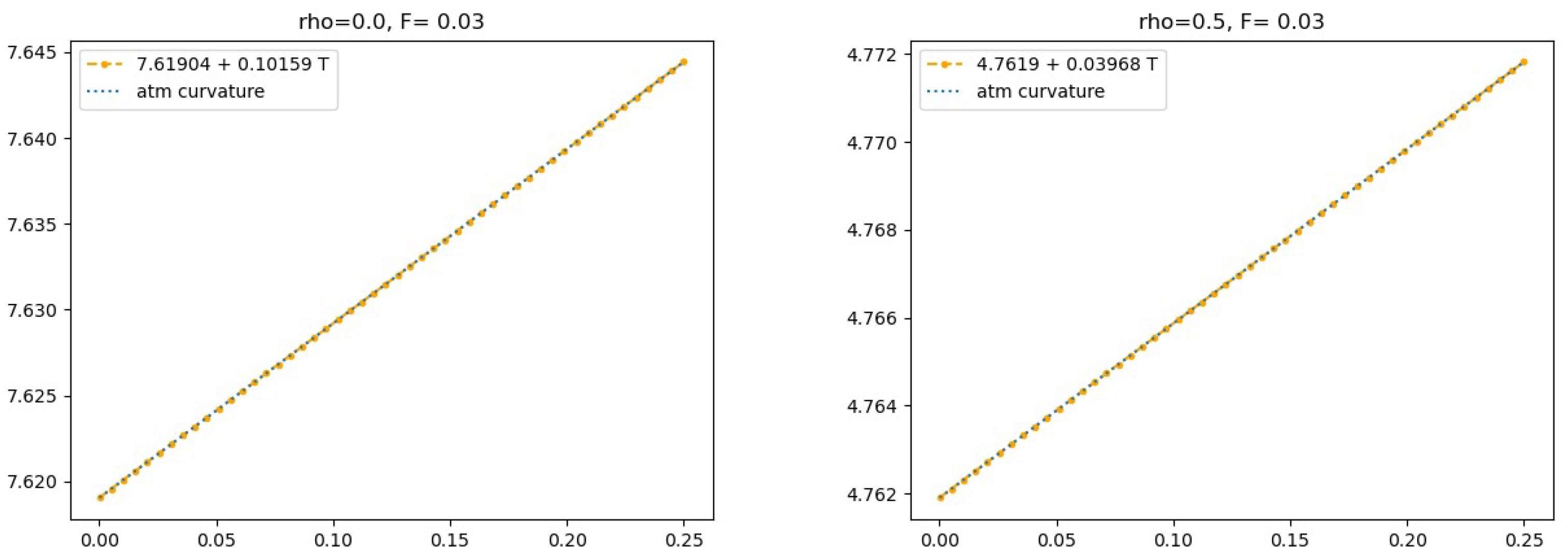
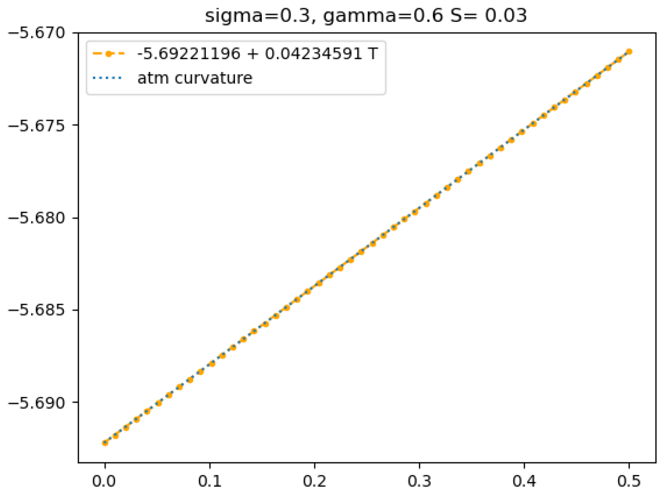
8. Examples

Let us see how the above results apply to some classical examples

Example 3. 

Let us consider a Bachelier–SABR model of the form

$$d{S}_t={\sigma }_t(\rho d{W}_t+\sqrt{1-{\rho }^2})d{B}_t$$

where σ is a geometric Brownian motion. That is,

$$d{\sigma }_t=\nu {\sigma }_{t}d{W}_t$$

Then, a straightforward computation leads to

$$D_s^W{\sigma }_t=\nu {\sigma }_t,$$

and

$$D_r^W{D}_s^W{\sigma }_t={\nu }^2{\sigma }_t,$$

for $r,s>t$. Then, Theorem 4 demonstrates that

$$\underset{T\to t}{lim}{\displaystyle \frac{{\partial }^{2}I}{\partial k^2}}(t,k_t^{*})=\left({\displaystyle \frac{1}{3}}-{\displaystyle \frac{1}{2}}{\rho }^2\right){\displaystyle \frac{{\nu }^2}{{\sigma }_t}}.$$

(33)

Notice that this expression can be positive or negative, depending on the correlation parameter. We can see this behaviour in the following plots, corresponding to a SABR model with $F_0=0.03$, $\nu =0.4,{\sigma }_0=0.07$, and $\rho =0$ (left) and $\rho =0.5$ (right). Note that if $\rho =0$, the above expression reduces to

$${\displaystyle \frac{1}{3}}{\displaystyle \frac{{\alpha }^2}{{\sigma }_t}}={\displaystyle \frac{0.4^2}{3\times 0.007}}=7.619,$$

while in the case where $\rho =0.5$ the curvature limit is

$$\left({\displaystyle \frac{1}{3}}-{\displaystyle \frac{1}{2}}0.5^2\right){\displaystyle \frac{0.4^2}{0.007}}=4.7619,$$

according to the results in Figure 1.

Figure 1. Implied volatility curvature as a function of time, for a SABR model with $\rho =0$ (left) and $\rho =0.5$ (right). Notice that the limits coincide with the computations in the text.

Example 4. 

Let us consider a Black–Scholes model:

$$d{S}_t=\sigma S_{t}d{W}_t,$$

for a constant σ. Notice that we can see this model as a Bachelier-type model with volatility ${\sigma }_t=\sigma S_t$. As

$$S_t=exp\left(-{\displaystyle \frac{{\sigma }^2}{2}}+\sigma W_t\right),$$

a direct computation leads to $D_r{S}_t=\sigma S_t$ and $D_r{D}_u{S}_t={\sigma }^2{S}_t$ (and then $D_r{\sigma }_t=\sigma {\sigma }_t$ and $D_r{D}_u{S}_t={\sigma }^2{\sigma }_t$), for $r,u<t$. This, in particular, implies that the Malliavin derivatives of ${\sigma }_t$ satisfy the required boundedness hypotheses with $H={\displaystyle \frac{1}{2}}$. Moreover,

$$D_s{M}_T={\int }_s^T{D}_s{\sigma }_r^{2}dr=2{\int }_s^T{\sigma }_r{D}_s{\sigma }_{r}dr=2\sigma {\int }_s^T{\sigma }_r^{2}dr,$$

and then,

$$D_s{D}_u{M}_T=4{\sigma }^2{\int }_s^T{\sigma }_r^{2}dr,$$

for $u<s<T$. Moreover,

$$\begin{array}{ccc}\hfill D_s\left({\sigma }_r{D}_u{M}_T\right)& =& \sigma {\sigma }_r{D}_u{M}_T+{\sigma }_r{D}_s{D}_u{M}_T\hfill \\ & =& 2{\sigma }^2{\sigma }_r{\int }_s^T{\sigma }_s^{2}ds+4{\sigma }^2{\sigma }_r{\int }_s^T{\sigma }_r^{2}dr\hfill \\ & =& 6{\sigma }^2{\sigma }_r{\int }_s^T{\sigma }_s^{2}ds\hfill \end{array}$$

(34)

Then, Theorem 4 allows us to write

$$\begin{array}{ccc}& & \underset{T\to t}{lim}{\displaystyle \frac{{\partial }^2{I}^{Bac}}{\partial k^2}}\left(k_t^{*}\right)\hfill \\ & & ={\displaystyle \frac{1{\sigma }^2}{{\sigma }_t}}{\displaystyle \frac{\left[{\int }_t^T{\left(T-r\right)}^{2}dr\right]}{{(T-t)}^3}}\hfill \\ & & +{\displaystyle \frac{1}{{\sigma }_t^5}}\left[-{\displaystyle \frac{6{\sigma }^2{\sigma }_t^4}{{\left(T-t\right)}^4}}{\left({\int }_t^T(T-s)ds\right)}^2+{\displaystyle \frac{6{\sigma }^2{\sigma }_t^4}{{\left(T-t\right)}^3}}{\int }_t^T{\int }_r^T(T-s)dsdr\right]\hfill \\ & & ={\displaystyle \frac{{\sigma }^2}{3{\sigma }_t}}-{\displaystyle \frac{3}{2}}{\displaystyle \frac{{\sigma }^2}{{\sigma }_t}}+{\displaystyle \frac{{\sigma }^2}{{\sigma }_t}}\hfill \\ & & ={\displaystyle \frac{{\sigma }^2}{{\sigma }_t}}\left({\displaystyle \frac{1}{3}}-{\displaystyle \frac{3}{2}}+1\right)\hfill \\ & & =-{\displaystyle \frac{\sigma }{6S_t}},\hfill \end{array}$$

which implies that, in the short-end limit, the Bachelier implied volatility of the Black–Scholes model is concave at the ATM strike.

Example 5. 

In this example, we compare (33) and derive the normal SABR formula with respect to strike. Afterward, we take $T\to 0$ under different scenarios of vol-of-vol (ν) and correlation (ρ). The normal SABR formula used is

$${\sigma }_{Hagan}(T,K)=\alpha {\displaystyle \frac{f\left(z\right)}{z}}{\displaystyle \frac{(1+{\nu }^{2}T(2-3{\rho }^2))}{24}},$$

where $z={\displaystyle \frac{\nu (S_0-K)}{\alpha }}$ and $f\left(z\right)=log\left(\sqrt{1-2\rho z+z^2}\right)$. The results obtained are shown in the following Table 1

Table 1. Hagan’s curvature vs. Malliavin ATM short-term limit.

$\mathit{\rho }$/$\mathit{\nu }$	0.1	0.25	0.4	0.55	0.7
−0.5	0.104/0.104	0.651/0.651	1.667/1.667	3.152/3.151	5.105/5.104
−0.3	0.144/0.144	0.901/0.901	2.307/2.307	4.362/4.361	7.067/7.064
0.0	0.167/0.167	1.042/1.042	2.667/2.667	5.043/5.042	8.17/8.167
0.3	0.144/0.144	0.901/0.901	2.307/2.307	4.362/4.361	7.067/7.064
0.5	0.104/0.104	0.651/0.651	1.667/1.667	3.152/3.151	5.105/5.104

Example 6. 

Let us consider a CEV model:

$$d{S}_t=\sigma S_t^{\gamma }d{W}_t,$$

for the constants $\sigma >0$ and $0<\gamma <1$. Notice that we can see this model as a Bachelier-type model with volatility ${\sigma }_t=\sigma S_t^{\gamma }$. Equality (8) allows us to see that

$$D_u{S}_t=\sigma S_u^{\gamma }+{\int }_u^t\gamma \sigma S_t^{\gamma -1}{D}_{u}Srd{W}_r,$$

(35)

which implies that

$$\underset{r\to t}{lim}{D}_r{S}_t=\sigma S_t^{\gamma }={\sigma }_t.$$

In the same way, we can find that

$$\underset{r\to t}{lim}{D}_r{\sigma }_t=\sigma \gamma {\sigma }_t{S}_t^{\gamma -1}.$$

Then, if we use the above equalities, we can show that the terms of Theorem 4 with $H={\displaystyle \frac{1}{2}}$ and $\rho =1$ are

$$\begin{array}{cc}\hfill {\displaystyle \frac{1}{4{\sigma }_t^5}}\underset{T\to t}{lim}{\displaystyle \frac{\left[E_t{\int }_t^T{\left(E_r\left(D_r^W{M}_T\right)\right)}^{2}dr\right]}{{(T-t)}^3}}& ={\displaystyle \frac{\sigma {\gamma }^2}{3}}{S}_t^{\gamma -2}\hfill \\ \hfill {\displaystyle \frac{1}{{\sigma }_t^5}}\underset{T\to t}{lim}{E}_t\left[-{\displaystyle \frac{3}{2{\left(T-t\right)}^4}}{\left({\int }_t^T{D}_s^W{M}_{T}ds\right)}^2\right]& ={\displaystyle \frac{-3\sigma {\gamma }^2}{2}}{S}_t^{\gamma -2}\hfill \\ \hfill \underset{T\to t}{lim}{E}_t\left[{\displaystyle \frac{1}{{\left(T-t\right)}^3}}{\int }_t^T\left({\int }_s^T{D}_s^W\left({\sigma }_r{D}_r^W{M}_T\right)dr\right){\sigma }_{s}ds\right]& =\sigma {\gamma }^2{S}_t^{\gamma -2}(1+{\displaystyle \frac{\gamma -1}{3\gamma }}).\hfill \end{array}$$

Therefore, we know that

$$\underset{T\to t}{lim}{\displaystyle \frac{{\partial }^2{I}^{Bac}}{\partial k^2}}\left(k_t^{*}\right)=\sigma {\gamma }^2{\displaystyle \frac{\gamma -2}{6\gamma }}{S}_t^{\gamma -2}.$$

In order to check the above limit, we use the Bachelier implied volatility approximation suggested by the authors in Hagan et al. (2002), applying the limit as $\nu \to 0$, i.e.,

$$I_{CEV}(t,T,k)=\sigma (S_t-K){\displaystyle \frac{1-\gamma }{S_t^{1-\gamma }-k^{1-\gamma }}}\left(1+(T-t){\displaystyle \frac{\gamma (\gamma -2){\sigma }^2}{24S_{t,avg}^{2(1-\gamma )}}}\right)$$

(36)

with $S_{t,avg}={\displaystyle \frac{S_t+k}{2}}$. Then, if we compute ${\partial }_{kk}$ of the above equation and we take $k\to S_t$ and $T\to t$, we obtain that

$$\underset{T\to t,k\to S_t}{lim}{I}_{CEV}(t,T,k)=\sigma {\gamma }^2{\displaystyle \frac{\gamma -2}{6\gamma }}{S}_t^{\gamma -2}.$$

Figure 2 presents the above results in a more visual way. We used $\sigma =0.3$ and $\gamma =0.6$. For this pair of parameters, we obtain that

$$\sigma {\gamma }^2{\displaystyle \frac{\gamma -2}{6\gamma }}{S}_0^{\gamma -2}=-5.69.$$

Figure 2. Curvature in the short term for the CEV model. Notice that the limit coincides with the computation in the text.

Example 7. 

In this example, we assume the same dynamics as in the above example, i.e.,

$$d{S}_t=\sigma S_t^{\gamma }d{W}_t,$$

In order to check the accuracy of Theorem 4 under different sets of parameters σ and γ, we create Table 2, where the results of computing the curvature using (36) and Theorem 4 are presented.

Table 2. CEV’s curvature vs. Malliavin ATM short-term limit.

$\mathit{\sigma }$/ $\mathit{\nu }$	0.01	0.015	0.02	0.025	0.03
0.1	−0.248/−0.248	−0.372/−0.372	−0.496/−0.496	−0.62/−0.619	−0.744/−0.743
0.2	−0.331/−0.331	−0.496/−0.496	−0.661/−0.661	−0.827/−0.827	−0.992/−0.992
0.3	−0.33/−0.33	−0.495/−0.495	−0.66/−0.66	−0.825/−0.825	−0.99/−0.99
0.4	−0.291/−0.291	−0.437/−0.437	−0.583/−0.583	−0.729/−0.729	−0.875/−0.874
0.5	−0.241/−0.241	−0.361/−0.361	−0.481/−0.481	−0.601/−0.601	−0.722/−0.722
0.6	−0.19/−0.19	−0.285/−0.285	−0.379/−0.379	−0.474/−0.474	−0.569/−0.569
0.7	−0.145/−0.145	−0.217/−0.217	−0.29/−0.29	−0.362/−0.362	−0.434/−0.434
0.8	−0.108/−0.108	−0.161/−0.161	−0.215/−0.215	−0.269/−0.269	−0.323/−0.323
0.9	−0.078/−0.078	−0.117/−0.117	−0.156/−0.156	−0.195/−0.195	−0.234/−0.234
0.95	−0.066/−0.066	−0.099/−0.099	−0.132/−0.132	−0.165/−0.165	−0.198/−0.198

9. Conclusions

By means of Malliavin calculus, we have proven an expression for the short-end curvature of the at-the-money Bachelier implied volatility. In particular, we have proven that this curvature is of the order $O\left(T^{2H-1}\right)$, where H is the Hurst parameter of the model. Moreover, our results prove that, for the CEV model, this curvature is negative if $\gamma <2$, while for the Bachelier–SABR model, this curvature can be positive or negative, depending on the correlation parameter.

References

- Alòs, Elisa, and David García-Lorite. 2023. Malliavin Calculus in Finance. Theory and Practice, 2nd ed. London: Chapman and Hall. [Google Scholar]
- Alòs, Elisa, and Jorge A. León. 2017. On the curvature of the smile in stochastic volatility models. SIAM Journal on Financial Mathematics 8: 373–99. [Google Scholar] [CrossRef]
- Alòs, Elisa, Eulalia Nualart, and Makar Pravosud. 2023. On the Implied Volatility of Asian Options Under Stochastic Volatility Models. Applied Mathematical Finance 30: 249–74. [Google Scholar] [CrossRef]
- Bachelier, Louis. 1900. Théorie de la spéculation. Annales scientifiques de l’École Normale Supérieure. Paris: Société Mathématique de France, Série 3, Tome 17. [Google Scholar]
- Choi, Jaehyuk, Minsuk Kwak, Chyng Wen Tee, and Yumeng Wang. 2022. A Black–Scholes user’s guide to the Bachelier model. Journal of Futures Markets 42: 959–80. [Google Scholar] [CrossRef]
- Gatheral, Jim. 2006. The Volatility Surface. A Practitioner’s Guide. New York: John Wiley and Sons. [Google Scholar]
- Hagan, Patrik, Andrew Lesniewski, and Diana Woodward. 2002. Managing Smile Risk. Wilmott Magazine 1: 84–102. [Google Scholar]
- Medvedev, Alexei, and Oliver Scaillet. 2007. Approximation and calibration of short-term implied volatilities under jump-diffusion stochastic volatility. Review of Financial Studies 20: 427–59. [Google Scholar] [CrossRef]
- Nualart, David. 2006. Probability and its Applications. In The Malliavin Calculus and Related Topics, 2nd ed. Berlin: Springer. [Google Scholar]
- Nualart, David, and Étienne Pardoux. 1988. Stochastic calculus with anticipating integrands. Probability Theory and Related Fields 78: 535–81. [Google Scholar] [CrossRef]
- Schachermayer, Walter, and Josef Teichmann. 2008. How close are the option pricing formulas of bachelier and black–merton–scholes? Mathematical Finance 18: 155–70. [Google Scholar] [CrossRef]
- Terakado, Satoshi. 2019. On the Option Pricing Formula Based on the Bachelier Model. Available online: https://papers.ssrn.com/sol3/papers.cfm?abstract_id=3428994 (accessed on 24 October 2024).