Quantum Majorization in Market Crash Prediction

Abstract

We introduce the Quantum Alarm System, a novel framework that combines the informational advantages of quantum majorization applied to tail pseudo-correlation matrices with the learning capabilities of a reinforced urn process, to predict financial turmoil and market crashes. This integration allows for a more nuanced analysis of the dependence structure in financial markets, particularly focusing on extreme events reflected in the tails of the distribution. Our model is tested using the daily log-returns of the 30 constituents of the Dow Jones Industrial Average, spanning from 2 January 1992 to 30 August 2024. The results are encouraging: in the validation set, the 12-month ahead probability of correct alarm is between $73\%$ and $80\%$, while maintaining a low false alarm rate. Thanks to the application of quantum majorization, the alarm system effectively captures non-traditional and emerging risk sources, such as the financial impact of the COVID-19 pandemic—an area where traditional models often fall short.

1. Introduction

Forecasting techniques have been widely applied to stock markets, yielding highly variable results, and attempting to give a comprehensive overview here would be nothing short of quixotic. Nonetheless, as expertly summarized in (Petropoulos et al. 2022), the bulk of these efforts has focused on modeling interest rates, asset returns, and changes in volatility. While asset returns have proven notoriously difficult to predict (Embrechts et al. 2003; McNeil et al. 2015; Rapach et al. 2010), volatility modeling has shown promise, particularly through realized volatility models (e.g., Taylor 2008) and the extensive literature stemming from the famous autoregressive conditional heteroscedastic (ARCH) approach (e.g., Bollerslev 1987; R. Engle 2004; R. F. Engle 1982). When it comes to interest rates, Markov switching models (e.g., Ang and Bekaert 2002; Haas et al. 2004; Hamilton 1988) and threshold (nonlinear) models (e.g., Gospodinov 2005; Pfann et al. 1996) have shown reasonable potential. However, out-of-sample performance, particularly for short rates, remains far from ideal (Brigo and Mercurio 2013; Homer and Sylla 1996; Oosterlee and Grzelak 2019; Petropoulos et al. 2022).

The literature on predicting market crashes—sudden and severe declines in stock prices that impact large portions, if not the entirety, of the market and result in significant financial losses—is relatively scarce (Claessens and Kose 2013). In (Sornette 2003, 2017) and (Sornette and Johansen 2006), the authors identify several potential causes of market crashes, such as illiquidity (notably seen in the 2007–2008 crisis and liquidity black holes Hull 2023), herding behavior (e.g., Park and Sabourian 2011), and unchecked securitization (Keys et al. 2009). The main approaches for forecasting the likelihood of a crash within a specific time horizon typically involve self-exciting jump processes and autoregressive conditional duration models. The former includes works like (Aït-Sahalia et al. 2015; Chavez-Demoulin et al. 2005), as well as promising studies utilizing Hawkes processes (e.g., Gresnigt et al. 2015; Hawkes 2022; Souto Arias et al. 2025). For the latter, the work of (Engle and Russell 1997, 1998), among others, is notable.

In this paper, we introduce a novel method for modeling the likelihood—and thus the potential occurrence—of market crashes, and more in general financial turmoil, over a specified time horizon. We propose an alarm system (De Maré 1980; Lindgren 1980) that combines quantum majorization (Fontanari et al. 2020) with the reinforced urn processes of (Muliere et al. 2000, 2003), building on the ideas presented in (Cirillo et al. 2013) and (Fontanari et al. 2020). We call this new model the “Quantum Alarm System”.

Leveraging quantum majorization (Section 2.2), we can encapsulate market risk, as well as non-traditional risk sources like pandemics, by constructing a sequence of pseudo-correlation matrices over a given time horizon. This sequence generates a time series of risk levels that is used to train a reinforced urn process (RUP)—a reinforced random walk on a state space of urns (Fortini and Petrone 2012)—which can then be applied for predictive purposes. An optimal alarm system is constructed by analyzing the probability of a market crash occurring over a set period, as predicted by the RUP. Following the methodology of (Sornette and Johansen 2006), we define financial turmoil when a drawdown with a magnitude of $12\%$ or more is observed. An alarm is triggered whenever the predicted probability of such an event exceeds a predefined threshold (Section 4).

The use of quantum majorization and its derived risk measures to study financial turmoil has shown interesting results when tested on data (Fontanari et al. 2020; Lanfranchi 2022). In this paper, we extend the analysis to the daily log-returns of the 30 Dow Jones Industrial Average (DJIA) constituents, spanning a 32-year period (1992–2024). The findings are intriguing and indicate that urn-based alarm systems combined with quantum majorization offer compelling paths for future research. The Quantum Alarm System, in particular, demonstrates the capacity to capture the impact of non-traditional risk sources on portfolios, especially when these portfolios are granular and representative of the market. This capability stems from its ability to extract information from pseudo-correlation matrices without the need to explicitly identify specific stressors, such as climate events, pandemics, or others.

The paper is structured as follows: Section 2 introduces the necessary tools to construct the quantum alarm system detailed in Section 3; Section 4 explains how the alarm system can be applied to real-world data and calibrated; Section 5 evaluates the system’s performance on the DJIA dataset; and Section 6 concludes the paper.

2. Methods

2.1. Alarm Systems

An alarm system is a probabilistic tool that predicts the occurrence of a given event at a specified time in the future on the basis of the available information. An alarm system is usually meant to activate when the probability of the event of interest in a given time horizon passes a certain threshold of tolerance (Lindgren 1980). In the financial literature, alarm systems are also known as early warning systems, or EWSs (Alessi and Detken 2011).

Let $\left\{X_t\right\}$ be a stochastic process with parameter space $\theta \in {\mathbb{R}}^d$, with d fixed. For some $q>0$, we divide the time sequel $\{1,\dots ,t-1,t,t+1,\dots \}$ into three intuitive sections: the past $\{1,\dots ,t-q\}$, the present $\{t-q+1,\dots ,t\}$, and the future $\{t+1,\dots \}$. Hence, we have that ${\mathbf{X}}_1=\{X_1,\dots ,X_{t-q}\}$, ${\mathbf{X}}_2=\{X_{t-q+1},\dots ,X_t\}$ and ${\mathbf{X}}_3=\{X_{t+1},\dots \}$ represent, respectively, the informative past, the present, and the future at time t.

The event of interest $E_{t+j}$ is an element in $\sigma \left({\mathbf{X}}_3\right)$, with the $\sigma$-algebra generated by ${\mathbf{X}}_3$. Without loss of generality, the event is assumed to occur in j steps from time t. Even if $E_{t+j}$ can be any event, it is usually seen as a rare event, i.e., an event whose occurrence in time is not common (Embrechts et al. 2003; Hüsler and Schmidt 1996).

An event $A_t\in \sigma \left({\mathbf{X}}_2\right)$ is an alarm for $E_{t+j}\in \sigma \left({\mathbf{X}}_3\right)$ if, whenever ${\mathbf{x}}_2\in A_t$, it is likely that $E_{t+j}$ takes place, i.e., $\mathbb{P}\left(E_{t+j}\right|A_t)\ge \gamma$, where $\gamma \in [0,1]$ is a threshold value, which can be subjective and predetermined, or data-driven.

We say that an alarm is cast at time t for a future event $E_{t+j}$ if the observed value ${\mathbf{x}}_2$ of ${\mathbf{X}}_2$ belongs to the predictor event. If an event of interest occurs after an alarm is given, the event is detected. If, on the contrary, it does not occur, we would have a false alarm.

In (De Maré 1980), an alarm system is considered optimal when, for a given set of available data, it achieves the highest probability of correctly signaling an alarm. This implies that, when the alarm is triggered, the likelihood that the event of interest will actually occur is the highest compared to all other possible systems.

As outlined in (Monteiro et al. 2008), a naive alarm system is represented by the predictor ${\widehat{X}}_{t+h}=\mathbb{E}\left[X_{t+h}\right|X_s,-\infty <s\le t,h>0]$, where an alarm is cast every time the predictor exceeds some risk level. Naturally this system is not optimal at all, because, as shown in (De Maré 1980), it does not provide good performance in detecting exceedances, in correctly locating exceedances in time, or in reducing the number of false alarms.

The principles of optimal prediction in level crossings for continuously valued processes have been outlined in (De Maré 1980; Lindgren 1975; Svensson et al. 1996). Appealing Bayesian approaches have been proposed in (Cirillo et al. 2013; Turkman and Turkman 1990). In (Antunes et al. 2003), results for autoregressive models of order k are discussed.

For the discrete case, results can be found, for example, in (Monteiro et al. 2008; Zheng et al. 2006). In particular, in (Monteiro et al. 2008), an alarm system that predicts whether or not a counting process will upcross a certain threshold has been developed.

Models relying on statistical learning are also increasingly common (Chen et al. 2021; Grage et al. 2010; Holopainen and Sarlin 2017; Qin et al. 2017; Sarlin and Peltonen 2013). In (Makridakis et al. 2018; Petropoulos et al. 2022), a comprehensive discussion on the topic can be found.

For a thorough review of the literature related to alarm systems, we refer to (Antunes et al. 2003; Grage et al. 2010; Monteiro et al. 2008; Zheng et al. 2006). For some appealing recent results, we suggest (Chen et al. 2021) and the references therein. The problems of forecasting and alarm systems for fat-tailed events have been recently discussed in (Taleb et al. 2020).

As pointed out in (De Maré 1980), in developing an alarm system, one is interested in the following operating characteristics: the alarm size $\mathbb{P}\left(A_t\right|{\mathbf{X}}_1)$; the probability of detecting the event $\mathbb{P}\left(E_{t+j}\right|A_t,{\mathbf{X}}_1)$; the probability of a correct alarm $\mathbb{P}\left(A_t\right|E_{t+j},{\mathbf{X}}_1)$; the probability of a false alarm $\mathbb{P}\left(A_t\right|E_{t+j}^c,{\mathbf{X}}_1)$; and the probability of an undetected event $\mathbb{P}\left(E_{t+j}\right|A_t^c,{\mathbf{X}}_1)$.

2.2. Quantum Majorization and the Measure $\theta$

Originally developed in the field of statistical physics to study entropy-increasing dynamics on Hermitian density matrices with equal trace (Alberti and Uhlmann 1982), Quantum Majorization (QM) was proposed in (Fontanari et al. 2020) as a partial order in the space of financial correlation matrices, to rank and compare them, with interesting insights in terms of their inherent risk.

Studied by Pólya and Schur among others (Hardy et al. 1952; Olkin and Marshall 2016), majorization is a way to define a partial order in the space of vectors in ${\mathbb{R}}^n$, ranking them in terms of their variability with respect to their common vector of averages.

Given a vector $\mathbf{x}=[x_1,x_2,\dots ,x_n]\in {\mathbb{R}}^n$, such that ${\sum }_{i=1}^n{x}_i=d$, the vector of averages is defined as

$$\overline{\mathbf{x}}=\left[{\displaystyle \frac{{\sum }_{i=1}^n{x}_i}{n}},\dots ,{\displaystyle \frac{{\sum }_{i=1}^n{x}_i}{n}}\right]=\left[{\displaystyle \frac{d}{n}},\dots ,{\displaystyle \frac{d}{n}}\right],$$

which is the n-dimensional vector whose entries correspond to the average of $\mathbf{x}$.

Now, take two vectors $\mathbf{x},\mathbf{y}\in {\mathbb{R}}^n$. We say that $\mathbf{x}$ majorizes $\mathbf{y}$, in symbols $\mathbf{x}\succ \mathbf{y}$, if

$$\sum _{i=1}^n{x}_i=\sum _{i=1}^n{y}_i,$$

(1)

and

$$\sum _{i=1}^k{x}_{\left[i\right]}\ge \sum _{i=1}^k{y}_{\left[i\right]},\mathrm{for}\mathrm{all}k=\{1,\dots ,n-1\},$$

(2)

where $x_{\left[1\right]},\dots ,x_{\left[n\right]}$ are the coordinates of the vector $\mathbf{x}$ sorted in descending order, so that $x_{\left[1\right]}\ge x_{\left[2\right]}\ge \dots \ge x_{\left[n\right]}$.

Since it represents a partial order (Arnold and Sarabia 2018), sometimes it is not possible to verify the majorization for $\mathbf{x}$ and $\mathbf{y}$. In these cases, one writes $\mathbf{x}\nsucc \mathbf{y}$. In all situations, however, majorization respects the transitivity property: if $\mathbf{x}\succ \mathbf{y}$ and $\mathbf{y}\succ \mathbf{z}$, then $\mathbf{x}\succ \mathbf{z}$.

Strictly related to majorization is the class of Schur-convex functions (Arnold and Sarabia 2018). These functions have the property of preserving the majorization property.

Consider a real-valued function $\varphi$ defined on ${\mathbb{R}}^n$. The function $\varphi$ is Schur-convex if, whenever $\mathbf{x}\succ \mathbf{y}$, $\varphi \left(\mathbf{x}\right)\ge \varphi \left(\mathbf{y}\right)$. When the inequality is strict, one has strictly Schur-convexity. If $\mathbf{x}\succ \mathbf{y}$ and $\varphi \left(\mathbf{x}\right)\le \varphi \left(\mathbf{y}\right)$, then $\varphi$ is Schur-concave, meaning that $-\varphi$ is Schur-convex.

Schur-convex functions can thus be used as summary measures of the variability of a vector, when variability is defined in terms of majorization. Interestingly, several quantities commonly employed in statistics to represent variability are Schur-convex, and therefore related to majorization: the variance, the coefficient of variation, the entropy, the mean absolute deviation, and inequality indices like the Gini and the Pietra (Arnold and Sarabia 2018; Hardy et al. 1952). Additionally, quantities like the arithmetic and the geometric means are Schur-convex.

Consider now a market portfolio $\mathcal{P}$ with n assets, whose values evolve over a time horizon $[0,T]$, which we split into k possibly overlapping intervals of equal length. Let ${\mathbf{C}}_i$ be the $n\times n$ pseudo-correlation matrix representing the dependence structure in $\mathcal{P}$ in time window $i=1,\dots ,k$. The matrix ${\mathbf{C}}_i$ is indeed a square, real-valued, Hermitian, and positive-semidefinite matrix, whose entries are correlation coefficients of any sort (Embrechts et al. 2003; Fontanari et al. 2020), typically lying in the interval $[-1,1]$, with all 1’s on the main diagonal.

In this work, also following (Montana 2021), we will rely on pseudo-correlation matrices built via the upper tail index of Gumbel copulas (more in Section 5). Alternative definitions of $\mathbf{C}$ can be (and have been) used, but the one based on the upper tail index shows the best performance for our data.

We say that ${\mathbf{C}}_i$ quantum majorizes ${\mathbf{C}}_j$, or in symbols ${\mathbf{C}}_i{\succ }^{\lambda }{\mathbf{C}}_j$ with $i,j\in \{1,\dots ,k\}$, if the spectrum of ${\mathbf{C}}_i$ majorizes that of ${\mathbf{C}}_j$. Applying the definition of majorization, this happens when

$$\sum _{m=1}^k{\lambda }_m\left({\mathbf{C}}_i\right)\ge \sum _{m=1}^k{\lambda }_m\left({\mathbf{C}}_j\right),\forall k=1,\dots ,n,$$

where ${\lambda }_1\left({\mathbf{C}}_i\right),{\lambda }_2\left({\mathbf{C}}_i\right),\dots ,{\lambda }_n\left({\mathbf{C}}_i\right)$ are the eigenvalues of ${\mathbf{C}}_i$, ordered from the largest to the smallest, possibly repeating in case of an algebraic multiplicity larger than 1. Notice that, trivially, ${\sum }_{m=1}^n{\lambda }_m\left({\mathbf{C}}_i\right)={\sum }_{m=1}^n{\lambda }_m\left({\mathbf{C}}_j\right)$, and this equality is a fundamental condition for majorization to hold (Fontanari et al. 2020).

If ${\mathbf{C}}_i{\succ }^{\lambda }{\mathbf{C}}_j$, then ${\mathbf{C}}_i$ can be perceived as riskier than ${\mathbf{C}}_j$, because the assets in portfolio $\mathcal{P}$ in period i show higher dependence than at time j, thus increasing portfolio risk and reducing diversification.

Notice that every correlation matrix ${\mathbf{C}}_i$ lives between two extremes: (1) the identity matrix $I_n$, corresponding to a portfolio of n independent assets, which is always majorized (maximal diversification), and (2) a rank-one matrix, corresponding to a portfolio in which all assets are (counter)comonotonic and there is no diversification (Fontanari et al. 2020). Finally, observe that, if ${\mathbf{C}}_i{\succ }^{\lambda }{\mathbf{C}}_j$ and ${\mathbf{C}}_j{\succ }^{\lambda }{\mathbf{C}}_i$, we can conclude that ${\mathbf{C}}_i$ and ${\mathbf{C}}_j$ have the same portfolio riskiness, but this does not mean that ${\mathbf{C}}_i={\mathbf{C}}_j$.

The use of eigensystems to study multivariate dependence has an important tradition, especially in finance: in the past decades, it has been shown that Markowitz-based portfolio optimization strategies are often outperformed by naive strategies such as the $1/N$ rule (DeMiguel et al. 2007; Duchin and Levy 2009). A reason for this is the instability of correlation matrix estimators, when the number of assets is large with respect to the length of the time series used for the estimation (Laloux et al. 1999). To resolve this, a number of different methodologies to build and study portfolios has been introduced, with many authors agreeing that eigenvalues-based strategies should be preferred (e.g., Laloux et al. 2000 and the references therein). Quantum majorization also appears as a promising tool in this setting (Fontanari et al. 2020).

Given a sequence ${\left\{{\mathbf{C}}_i\right\}}_{i=1}^k$ of correlation matrices, we define the $k\times k$ Quantum Majorization Matrix $\mathbf{A}$, where

$$A_{i,j}=\left\{\begin{array}{c}1\mathrm{if}{\mathbf{C}}_i{\succ }^{\lambda }{\mathbf{C}}_j\hfill \\ 0\mathrm{otherwise}\hfill \end{array}\right.,i,j=1,\dots ,k.$$

(3)

Figure 1 gives a graphical representations of a possible $8\times 8$ Quantum Majorization Matrix (QMM), collecting the majorization relations among eight different correlation matrices, each measuring the risk in a given portfolio (or index), in a particular time period $t=1,2,\dots ,8$. To represent the different $A_{i,j}$’s in the QMM, we choose black for 1, and white for 0. Yellow is used to indicate the trivial case of a correlation matrix majorizing and being majorized by itself.

Let us consider row $t=2$ in Figure 1, where we can read the quantum majorization relations of correlation matrix ${\mathbf{C}}_2$ with respect to the other matrices in the set. We see that cells $\{t=2,t=1\}$ and $\{t=2,t=8\}$ are black. This indicates that ${\mathbf{C}}_2$ majorizes both ${\mathbf{C}}_1$ and ${\mathbf{C}}_8$, suggesting that the overall risk embedded in ${\mathbf{C}}_2$ is higher than that in ${\mathbf{C}}_1$ and ${\mathbf{C}}_8$. At the same time, the other cells on the line are white (with the exception of the diagonal cell $\{t=2,t=2\}$), suggesting that the corresponding correlation matrices majorize ${\mathbf{C}}_2$. Summarizing: period $t=2$ can be considered riskier than $t=1$ or $t=8$, but it is less risky than $t=3$, $t=4$, and so on.

Always in Figure 1, we see that ${\mathbf{C}}_6$, represented by row $t=6$, majorizes all of the others, thus representing the up-to-date maximum in the set of correlation matrices, in terms of embedded risk. Matrix ${\mathbf{C}}_5$ then represents the second riskiest correlation matrix (up-to-date), which majorizes all others apart from the one represented by ${\mathbf{C}}_6$, by which it is majorized: ${\mathbf{C}}_6{\succ }^{\lambda }{\mathbf{C}}_5$.

Looking at patterns in a QMM, one can therefore identify periods of higher and lower risk, and compare them. We refer to (Fontanari et al. 2020) for further details.

From the Quantum Majorization Matrix $\mathbf{A}$, we can derive the risk measure $\theta :\mathbf{A}\to \mathbb{R}$, as

$$\theta \left({\mathbf{C}}_i\right)={\theta }_i={\displaystyle \frac{1}{2}}+{\displaystyle \frac{1}{2k}}\left(\sum _{j=1}^k{A}_{i,j}-\sum _{i=1}^k{A}_{j,i}\right)\in [0,1].$$

(4)

Equation (4) represents the risk embedded in a correlation matrix as a function of the total number of matrices by which it is quantum-majorized, and that it quantum-majorizes. Notice that $\theta \left({\mathbf{C}}_i\right)$ is order-preserving with respect to quantum majorization ($\theta$ is Schur-convex); therefore, if ${\mathbf{C}}_{\mathbf{i}}{\succ }^{\lambda }{\mathbf{C}}_{\mathbf{j}}$, then $\theta \left({\mathbf{C}}_{\mathbf{i}}\right)\ge \theta \left({\mathbf{C}}_{\mathbf{j}}\right)$.

The case ${\theta }_i=0$ indicates that ${\mathbf{C}}_i$ is quantum-majorized by all other matrices in the collection, while ${\theta }_i=1$ implies that ${\mathbf{C}}_i$ is the up-to-date riskiest matrix, which majorizes all the others. All intermediate levels allow us to assess and rank the riskiness of portfolio $\mathcal{P}$ in the different periods, as captured by the corresponding correlation matrix.

2.3. Reinforced Urn Processes

A Reinforced Urn Process (RUP) is a combinatorial stochastic process, introduced in (Muliere et al. 2000) as a random walk on a state space of urns. RUPs have been successfully applied to the modeling of several relevant phenomena in finance and risk management, e.g., (Cheng and Cirillo 2018; Peluso et al. 2015; Souto Arias and Cirillo 2021).

By adjusting the hyperparameters of a Reinforced Urn Process (RUP), one can derive a variety of nonparametric models, each with a machine learning or deep learning flavor. A RUP has indeed the ability to learn from data, continually updating its parameters and improving its performance over time. What distinguishes RUPs from other approaches is the ease with which prior knowledge can be incorporated, allowing the integration of expert judgment with empirical data. This feature makes RUPs particularly effective in handling missing data, identifying trends, and accounting for rare events, while also reducing historical biases (Cheng and Cirillo 2018). Unlike many deep learning models, where decision-making processes are often opaque, RUPs maintain transparency, avoiding the “black box” problem (Knight 2017).

In the following, we consider a state space $S={\mathbb{N}}_0^{+}\times \{1,2,3\}$, whose elements $s=(t,l)$ represent levels of risk l at (discrete) time points t. Level $l=1$ represents no or low risk of “catastrophe” (a little hyperbole for a market crash or a period of financial turmoil), $l=2$ a medium risk, and $l=3$ a high risk. Our goal will be to cast an alarm whenever the probability of reaching level 3 is above a certain safety threshold $\gamma$, to be defined later.

On every state $s\in S$, we center a different Polyá-like urn $U\left(s\right)$, i.e., an urn characterized by sampling with reinforcement (Mahmoud 2009). Every $U\left(s\right)$, $s\in S$, contains balls of 3 colors, $C=\{c_1,c_2,c_3\}$. The urn compositions can be different, but every urn contains at least one ball. In more detail, we assume all urns centered on states of the form $(t,1)$ not to contain balls of color $c_1$, while all other urns will contain at least a ball of each color.

We then define a function $q:S\times C\to S$ called a Rule of Motion (RoM), such that

$$q((t,l),c)=\left\{\begin{array}{cc}(t+1,l-1),\hfill & \mathrm{if}c=c_1\hfill \\ (t+1,l),\hfill & \mathrm{if}c=c_2\hfill \\ (t+1,l+1),\hfill & \mathrm{if}c=c_3\mathrm{and}l\ne 3\hfill \\ (t+1,l),\hfill & \mathrm{if}c=c_3\mathrm{and}l=3\hfill \end{array}\right..$$

(5)

Since the couple $(t,l)$ describes a risk level l at time t, the RoM q states that, when we are in $s=(t,l)$ and we sample a ball from $U\left(s\right)$, then, if the color is $c_2$, we move to $(t+1,l)$; i.e., as time passes, we stay at the same level of risk. If we pick $c_3$, the level of risk in the next time period increases by 1 (unless we are already in $l=3$). If $c_1$, the level of risk decreases by 1 (unless we are already in $l=1$). Since $U\left(s\right)$ is a Polyá-like urn, every time we sample a ball, we modify the composition of the urn by returning the ball and adding $\delta >0$ extra balls of the same color (Muliere et al. 2000).

We then define an RUP $Z_t$ as follows. We start from $Z_0=(0,1)$. For all $t\ge 1$, if $Z_{t-1}=s\in S$, a ball is sampled from $U\left(s\right)$, its color $c_i$ is registered, and $U\left(s\right)$ is Polyá reinforced with $\delta$ balls of the same color. We then apply the RoM q of Equation (5) to decide the next state that the process $Z_t$ will visit.

Consider a finite sequence $\mathbf{s}=\left(\right(0,1),\dots ,(i,j),\dots ,(t,l\left)\right)$ of elements of the state-space S. For the process $\left\{Z_t\right\}$, the sequence $\mathbf{s}$ is admissible (Diaconis and Freedman 1980) if, for any two adjacent states $(i,j)$ and $(i+1,k)$ in $\mathbf{s}$, there is at least one ball of color c in $U\left(\right(i,j\left)\right)$ such that $q\left(\right(i,j\left)\right),c)=(i+1,k)$. For example, in our model, a jump of 2 levels of risk in one step is not possible, so a sequence containing this would not be admissible.

Let ${\kappa }_s\left(c\right)$ be the number of balls of color c in urn $U\left(s\right)$. Let $f_s\left(c_i\right)$ be the function counting the number of transitions from state $s\in S$ to state $q(s,c_i)\in S$, and set $F\left(s\right)$ to be the total number of transitions from s to all other states present in $\mathbf{s}$.

The following theorem shows how to compute the probability of a given trajectory for the reinforced urn process described above.

Theorem 1.

For $t\ge 0$ and all finite sequences $\mathbf{s}=(s_0,\dots ,s_t)$ of elements in S, we have $\mathbb{P}[\left\{Z_t\right\}=\mathbf{s}]=0$, if $\mathbf{s}$ is not admissible, and

$$\mathbb{P}[\left\{Z_t\right\}=\mathbf{s}]=\prod _{s\in S}{\displaystyle \frac{{\prod }_{i=1}^3{\prod }_{j=0}^{f_s\left(c_i\right)-1}({\kappa }_s\left(c_i\right)+j\delta )}{{\prod }_{k=0}^{F\left(s\right)-1}\left({\sum }_{i=1}^3{\kappa }_s\left(c_i\right)+k\delta \right)}}$$

(6)

otherwise, with ${\prod }_0^{-1}(·)=1$.

Proof. 

The proof of the theorem mimics that in Muliere et al. (2000). Here we provide the main steps.

By definition, a not admissible sequence $\mathbf{s}$ cannot be visited by the RUP, so its probability is trivially null.

If $\mathbf{s}=(s_0,\dots ,s_t)$ is admissible, let $c(s_k,s_{k+1})$, $k=0,\dots ,t-1$, be the color ($c_1$,$c_2$, or $c_3$) of the ball such that, once extracted from the urn centered in $s_k$, allows the RUP to reach $s_{k+1}$. Then

$$P[Z_0=s_0,\dots ,Z_t=s_t]=\prod _{k=0}^{t-1}{\displaystyle \frac{{\kappa }_{s_k}\left(c(s_k,s_{k+1})\right)+m_{s_k}\left(c(s_k,s_{k+1})\right)}{{\sum }_{i=1}^3({\kappa }_{s_k}\left(c_i\right)+m_{s_k}\left(c_i\right))}},$$

(7)

where $m_{s_0}(·)\equiv 0$ and

$$m_{s_k}\left(c\right)=\delta \sum _{r=0}^{k-1}{1}_{\{s_r=s_k,c(s_r,s_{r+1})=c\}},$$

for $c\in \{c_1,c_2,c_3\}$, and $k=1,\dots ,t-1$.

Now, let an element s in the admissible sequence $\{s_0,\dots ,s_t\}$. Let $\{y_1,\dots ,y_{F\left(s\right)}\}$ be the ordered sequence of states that follow s in $\mathbf{s}$. The group of factors relative to s in Equation (7) can therefore be reformulated as

$$\begin{array}{c}\hfill {\displaystyle \frac{{\kappa }_s\left(c(s,y_1)\right)}{{\sum }_{i=1}^3{\kappa }_x\left(c_i\right)}}·{\displaystyle \frac{{\kappa }_s\left(c(s,y_2)\right)+\delta 1_{\{y_1=y_2\}}}{\delta +{\sum }_{i=1}^3{\kappa }_x\left(c_i\right)}}\cdots {\displaystyle \frac{{\kappa }_s\left(c(s,y_{F\left(s\right)})\right)+\delta {\sum }_{j=1}^{F\left(s\right)-1}{1}_{\{y_j=y_{F\left(s\right)-1}\}}}{\delta (F\left(s\right)-1)+{\sum }_{i=1}^3{\kappa }_x\left(c_i\right)}}\\ \hfill ={\displaystyle \frac{{\prod }_{i=1}^3{\prod }_{j=0}^{f_s\left(c_i\right)-1}({\kappa }_s\left(c_i\right)+j\delta )}{{\prod }_{k=0}^{F\left(s\right)-1}\left({\sum }_{i=1}^3{\kappa }_s\left(c_i\right)+k\delta \right)}},\end{array}$$

with the convention that ${\sum }_1^0·=0$.

By considering all possible states $s\in \mathbf{s}$, Equation (6) follows. □

As stated, an RUP is a process that can learn from data, but to do so we need some condition of recursiveness. In fact, if we can assure that the RUP may visit again a given state $s\in S$, then the previous samplings from $U\left(s\right)$ will impact our current probabilities of extracting $c_i$ from $U\left(s\right)$, $i=1,\dots ,3$. For example, if in a given state $(i,j)$ we have extracted a $c_1$ ball before, the chance of doing that again has increased, and so has the chance of moving to $(i+1,j-1)$.

Set ${\tau }_0=0$, and for $r\ge 1$ define ${\tau }_r=inf\{m>{\tau }_{r-1}|Z_m=s_0\}$. This way, $\left\{{\tau }_r\right\}$ represents the sequence of times elapsed between two consecutive visits of the (initial) state $s_0=(0,1)$ by $Z_t$. We say $\left\{Z_t\right\}$ is recurrent if $\mathbb{P}\left[{\cap }_{r=0}^{+\infty }\{{\tau }_t<+\infty \}\right]=1$.

An approach to force recursiveness is to reset $Z_t$ to $(0,1)$ every time one of the following two conditions verifies after reaching state $(t,3)$, i.e., reaching a catastrophe (we indicate the event $Z_t=(t,3)$ with $E_t$): 1) the process stays in level 3 because of w subsequent extractions of $c_3$ balls, or 2) a non-$c_3$ ball is sampled anytime thereafter.

As a consequence, the process $\left\{Z_t\right\}$ generates a sequence of so-called 0-blocks (Muliere et al. 2000): admissible sub-sequences starting with $(0,1)$ and ending in a state $(·,3)$, according to one of the conditions above.

Suppose $w=3$, and omit t for notational convenience. An example of a sequence of 0-blocks, in terms of risk levels l, can be

$$\stackrel{\mathrm{Block}1}{\overbrace{1,1,1,2,1,2,3,3}}|\underset{\mathrm{Block}2}{\underbrace{1,1,2,3,3,3,3}}|\stackrel{\mathrm{Block}3}{\overbrace{1,2,1,1,2,3}}$$

(8)

Block 1 tells us the RUP has visited states $\left(\right(0,1)$,$(1,1)$,$(2,1)$,$(3,2)$,$(4,1)$,$(5,2)$,$(6,3))$ and ultimately it is reset through the extraction of a non-$c_3$ colored ball in state $(7,3)$. Block 2 corresponds to $\left(\right(0,1),(1,1),(2,3),(3,3),(4,3),(5,3\left)\right)$ terminating after fulfilling the consecutive extraction of $w=3$ balls of color $c_3$ after state $(2,3)$. Finally, Block 3 refers to $\left(\right(0,1),(1,2),(2,1),(3,1),(4,2),(5,3\left)\right)$ and is terminated by the extraction of a non-$c_3$ ball after $(6,3)$.

A simple condition (Montana 2021) for recursiveness is given by

$$\underset{t\to +\infty }{lim}\prod _{j=0}^t{\displaystyle \frac{{\kappa }_{(j,l)}\left(c_1\right)+{\kappa }_{(j,l)}\left(c_2\right)}{{\sum }_{i=1}^3{\kappa }_{(j,l)}\left(c_i\right)}}=0.$$

(9)

We will not enter into the details here, but a recurrent RUP defines a conjugate process whose parameters are easily updated over time, without any necessity of re-training (Cirillo et al. 2013; Muliere et al. 2000), and one can show that the 0-blocks are exchangeable, so there is a de Finetti measure for the entire process (de Finetti 2017; Diaconis and Freedman 1980). These results will prove essential for the explainability and the interpretability of the model in future research on the topic.

3. The Quantum Alarm System

We now follow the suggestions in (Fontanari et al. 2020) and (Cirillo et al. 2013), and build an urn-based alarm system that combines QM and the RUP.

Assume that our process has observed $r-1$ catastrophes, i.e., it has reached level of risk 3, and it has been set again to $(0,1)$ following one of the reset rules, hence generating $r-1$ 0-blocks. We are interested in knowing when $\left\{Z_t\right\}$ will likely reach the next catastrophe E if at present we are in state $(t,l)$. We denote with

$$p_{t,h}^{*}=\mathbb{P}[{\tau }_r\in [t,t+h]|{\mathit{\tau }}_{r-1}],{\mathit{\tau }}_{r-1}=\{{\tau }_1,\dots ,{\tau }_{r-1}\}$$

(10)

the probability that there will be a catastrophe within k time steps from now.

Suppose there are m feasible paths, i.e., admissible sequences, between $(t,l)$ and $(t+h,3)$. Relying on Equation (6), we can compute $p_{t,h}^{*}$ as

$$p_{t,h}^{*}=\sum _{j=1}^h\sum _{i=1}^m\mathbb{P}[(t,l),\stackrel{i}{\overbrace{\dots }},(t+j,3)],$$

(11)

where $\mathbb{P}[(t,l),\stackrel{i}{\overbrace{\dots }},(n+j,3)]$ is the probability of the i-th feasible path from $(t,l)$ to $(t+j,3)$.

As shown in (Cirillo et al. 2013), an effective alarm system—called an urn-based alarm system—casts an alarm $A_t$, at time t, if the probability of a catastrophe in k steps exceeds a predetermined threshold $\gamma \in [0,1]$, i.e., for $p_{t,h}^{*}\ge \gamma$. The threshold $\gamma$ can be defined a priori, on the basis of specific knowledge, or it can be calibrated on a validation dataset, as to maximize the number of correct alarms, while minimizing the number of false alarms. We compute with $\mathbb{P}\left[E_{t+h}\right|A_t]$ the probability that an alarm accurately predicts a catastrophic event h steps ahead.

It is needless to say that computing $\mathbb{P}[{\tau }_r\in (t,t+h]|{\tau }_{r-1}]$ involves taking into account a number of paths that increases with h. As a consequence, large values of h can strongly affect the computational time needed to run the model. A combinatorial intuition is provided in (Cirillo et al. 2013), together with some heuristics.

Now, how can majorization and the urn-based alarm system be combined, thus creating the Quantum Alarm System?

Given a collection ${\mathbf{C}}_1,\dots ,{\mathbf{C}}_k$ of correlation matrices related to a portfolio $\mathcal{P}$ over time periods $1,\dots ,k$, we build the corresponding Quantum Majorization Matrix $\mathbf{A}$, from which we derive the sequence $\theta \left({\mathbf{C}}_1\right),\dots ,\theta \left({\mathbf{C}}_k\right)$ using Equation (4). Each $\theta \left({\mathbf{C}}_i\right)$ summarizes the riskiness of $\mathcal{P}$ during time period $i=1,\dots ,k$. We then discretize the values $\theta \left({\mathbf{C}}_i\right)$ by introducing three levels of risk: safe or low risk of catastrophe (1) if ${\theta }_i\in [0,{ϵ}_1)$, medium risk (2) when ${\theta }_i\in [{ϵ}_1,{ϵ}_2)$, and high risk (3) when $\theta \in [{ϵ}_2,1]$. In doing this, we generate a sequence of risk levels over time, where levels go from 1 to 3, and each time step corresponds to a time window for the underlying portfolio $\mathcal{P}$. On this sequence of couples $(t,l)$, we then impose the RUP process of Section 2.3. The thresholds ${ϵ}_1$ and ${ϵ}_2$ can be defined a priori, or calibrated to minimize the false alarms and maximize the correct ones, as we do here.

4. Data and Calculations

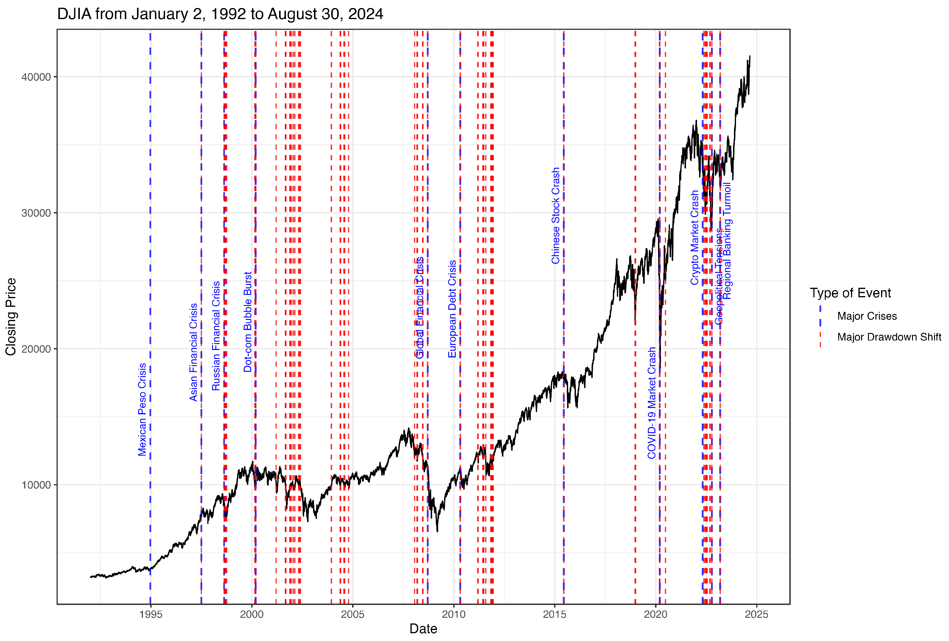
We analyze the daily log-returns of the 30 constituents of the Dow Jones Industrial Average (DJIA), spanning 8227 trading days between 2 January 1992 and 30 August 2024, as available from Yahoo! Finance. The time series of the DJIA (daily closing price) for the same time window is given in Figure 2. The plot also contains the major financial crises in the period (dashed blue lines), as commonly named by the media (e.g., Bloomberg 2024; International Banker 2024), together with the indication of the relevant drawdown shifts ($12\%$ or more) of the DJIA index (dashed red lines). It is interesting to observe that all major crises, except for the Mexican Peso Crisis of 1994–95 and the Crypto Market Crash of 2022, overlap and are preceded by major drawdown shifts in the DJIA. Figure 2 also shows how 2022 was a challenging year for financial markets, with a large number of major drawdown shifts. Similarly poor performances have only been observed during the 2007–2008 Global Financial Crisis over the past 20 years.

Using sliding windows of 100 days with 40-day shifts, we construct a sequence of 204 pseudo-correlation matrices, where each entry represents the upper tail dependence index $u(X_i,X_j)$ between two constituents, $X_i$ and $X_j$. Other combinations of window sizes (up to 150 days) and overlaps (between 10 and 90 days) were tested. As noted in (Fontanari et al. 2020), varying these parameters does not significantly affect the results, provided at least 50 correlation matrices can be generated. The 100/40 combination was also selected as an optimal balance for visualization purposes.

Given $X_i$ and $X_j$, we have

$$u(X_i,X_j)=\underset{p\to 1}{lim}\mathbb{P}(X_i>F_{X_i}^{-1}\left(p\right)|X_j>F_{X_j}^{-1}(p)),$$

where $F_{X_i}^{-1}\left(p\right)$ represents the generalized quantile function of $X_i$. Following the idea in (Montana 2021), we model the joint probability of each pair $(X_i,X_j)$ with a Gumbel copula (Nelsen 2006), i.e.,

$$C(v,w)=exp\left[-{\left({(-log\left(v\right))}^{\alpha }+{(-log\left(w\right))}^{\alpha }\right)}^{1/\alpha }\right],$$

with $v,w$ uniform margins and $\alpha \in [1,+\infty )$. The choice is based on preliminary empirical analyses of the DJIA data (Montana 2021), and is also in line with the literature (Malevergne and Sornette 2006). As a consequence, the upper tail dependence index becomes $u(X_i,X_j)=2-2^{1/\alpha }$, and its estimation is simple (Nelsen 1997).

Since u is symmetric, it lives in $[0,1]$, and clearly $u(X_i,X_i)=1$. The corresponding pseudo-correlation matrix $\mathbf{C}$ is a positive-semidefinite, real-valued, Hermitian matrix, on which we can apply quantum majorization.

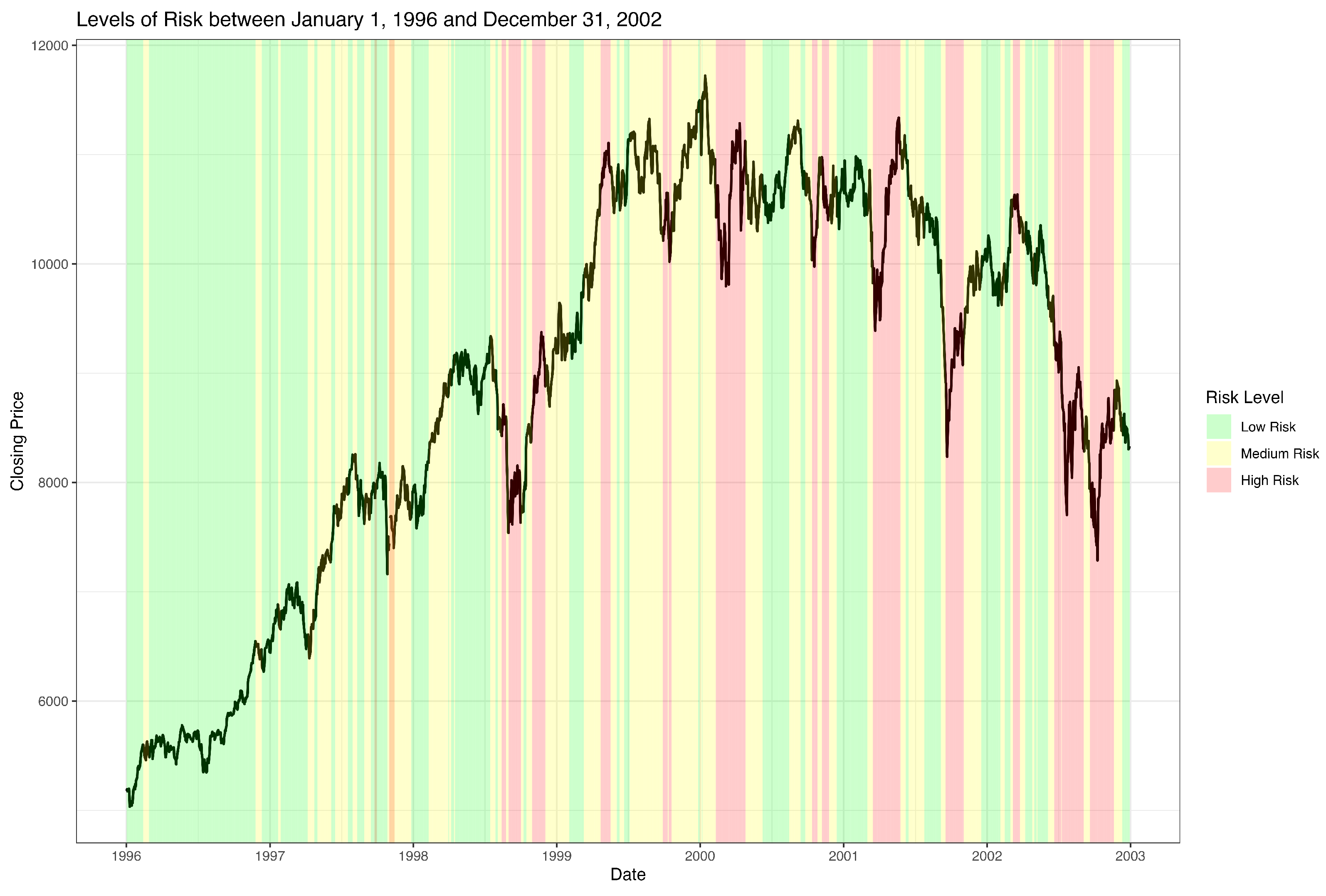
The risk-measure $\theta \left({\mathbf{C}}_i\right)$ of Equation (4) places each correlation matrix ${\mathbf{C}}_i$ into one of three risk levels: low ($\theta \left({\mathbf{C}}_i\right)<0.41={ϵ}_1$), medium ($0.41\le \theta \left({\mathbf{C}}_i\right)<0.80={ϵ}_2$), and high ($\theta \left({\mathbf{C}}_i\right)\ge 0.80$). These thresholds are the result of a calibration exercise (a basic grid search), meant to maximize the out-of-sample performances of the Quantum Alarm System (i.e., the maximization of the number of correct alarms, and the minimization of the false alarms). Figure 3 shows an excerpt of the DJIA time series of Figure 2, for the sub-period of 1 January 1996–31 December 2002. The levels of risk as measured by $\theta$ are shown as colored areas.

To first build and then evaluate the Quantum Alarm System, the data points have been split into a training part (2 January 1992–31 December 2018) and a validation part (1 January 2019–30 August 2024). The latter contains a series of 33 correlation matrices to play with. The split between training and validation shows that about $84\%$ of the observations are used to build the model and update its parameters, while the rest (about $16\%$) is used for the out-of-sample performance evaluation. In playing with the Quantum Alarm System, we have found that the performances of the model (see Section 5) remain relatively stable, as long as at least $80\%$ of the observations are used for training (more details in Section 5). Below this threshold, results deteriorate noticeably. Naturally, all of this is true for the DJIA data we are considering, and other optimal splits could emerge in other applications.

To define a catastrophe, we have used a $12\%$ or more drawdown shift in the DJIA time series, following (Montana 2021) and (Sornette and Johansen 2006). As already observed in Figure 3, major drawdown shifts are linked to most of the major financial crises in our dataset. The training dataset contains 45 major drawdown shifts, while 10 similar events are to be found in the validation dataset.

The use of the DJIA and its underlying constituents is convenient for two reasons. First, an index like the DJIA can be seen as a representative portfolio for a given (sub)market, so we can use it to look for financial turmoil on that market. Second, it is known that the stability of an empirical correlation matrix depends on the ratio between the number of variables n and the corresponding number of observations N used to construct the matrix (Zumbach 2011). If the ratio $n/N$ is not sufficiently small, the stability of $\mathbf{C}$ is not guaranteed. Using the DJIA, which consists of 30 assets (we could have alternatively used the CAC 40 or the DAX 30), provides a sufficiently small ratio for any reasonable sliding window of length N, as opposed to other indices such as the S&P500 or the FTSE100.

Both for training and validation, we have chosen three different values of the h-step ahead predictions on the $\theta$ time series: $h=2,4,6$, corresponding to approximately 4, 8, and 12 months, respectively, when looking at the original DJIA time series.

To train the Quantum Alarm System, we have initialized all urns with $c_1=30$, $c_2=55$, and $c_3=15$ (recall that all urns on level $l=1$ do not contain $c_1$ balls, so that for them $c_1=0$, $c_2=85$, and $c_3=15$). Without no particular prior information, these numbers reflect the idea that periods of financial turmoil are rare with respect to business. As discussed in (Muliere et al. 2000), in case of some more reliable prior beliefs, we could have incorporated them by further intervening on the urn compositions, allowing for the inclusion of plausible trends not present in the data. However, this was not our case.

We then considered the values $\theta \left({\mathbf{C}}_1\right),\dots ,\theta \left({\mathbf{C}}_k\right)$ and transformed the information into a sequence of couples $(t,l)$, using the thresholds ${ϵ}_1=0.41$ and ${ϵ}_2=0.80$ provided above.

Imagine that an excerpt of the sequence is given by

$$\cdots (3,1),(4,1),(5,2),(6,3)(0,1)\cdots ,$$

and that we see this as the result of the RUP from Section 2.3. We can easily derive that, in the urn centered in $(3,1)$, a $c_2$ ball has been selected, because the next state is $(4,1)$. Therefore, we update the composition of $U\left(\right(3,1\left)\right)$ with a number $\delta$ of $c_2$ balls as per

Table 1. Optimal hyper-parameters for the Quantum Alarm System, to maximize the probability of correct alarm detection.

Parameter	4-Month ($\mathit{h}=2$)	8-Month ($\mathit{h}=4$)	12-Month ($\mathit{h}=6$)
$\gamma$	$0.445$	$0.542$	$0.072$
$\delta$	7	8	2
w	0	0	2

and Equation (6). In $(4,1)$, conversely, a $c_3$ ball has been sampled (we move from $l=1$ to $l=2$), and we reinforce $c_3$ balls. After $(6,3)$, we observe $(0,1)$, indicating that the process has been reset, thus starting a new 0-block, and urn $U\left(\right(6,3\left)\right)$ is updated with $\delta$ balls of either $c_1$ or $c_2$ (coin toss). Doing this for all the data in the training set, the RUP parameters are updated.

As mentioned, an alarm is cast whenever $p_{t,h}^{*}\ge \gamma$, and the optimal in-sample values for $\delta$, $\gamma$ and the recurrence parameter w are obtained via a simple grid search to obtain ${\mathrm{argmax}}_{(\delta ,\gamma ,w)}\mathcal{P}\left[E_{t+h}\right|A_t]$, with $\gamma \in (0,1)$, $\delta ,w\in \{1,10\}$, for $h=2,4,6$. The results are in Table 1.

A few comments regarding the 12-month detection threshold are necessary. The value $\gamma =0.072$ is one order of magnitude lower than those used in the 4- and 8-month models. We believe this difference is due to the parameter $w=2$. In this context, the decrease from $0.542$ to $0.072$ is reasonable. When $w>0$, it leads to repeated multiplication of the probabilities of sampling $c_3$ balls, whose initial number in the urns is intentionally limited to prevent an a priori excessive occurrence of catastrophic events.

5. Results and Discussion

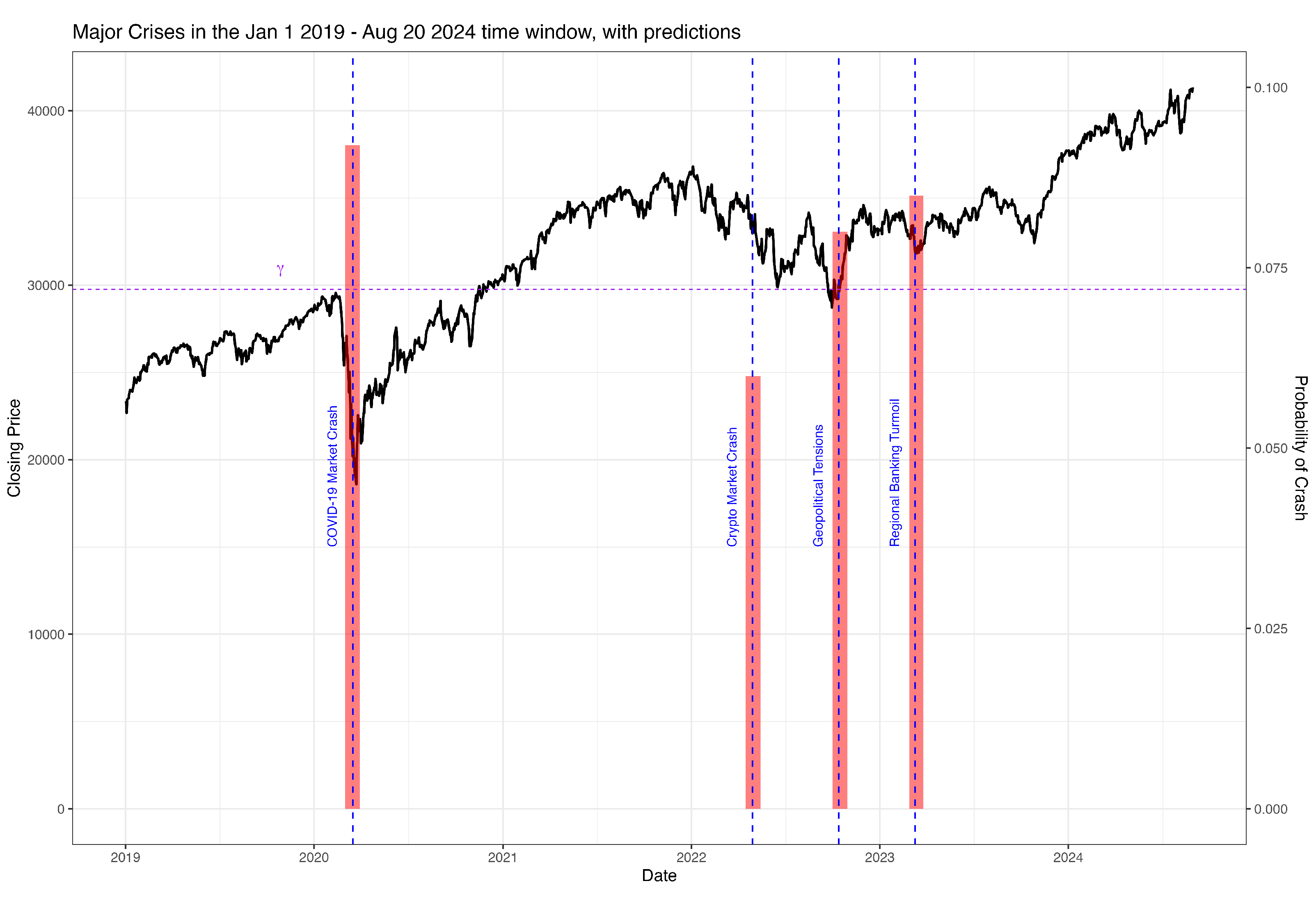
Figure 4 shows the daily log-returns of the Dow Jones Industrial Average from 1 January 2019 to 30 August 2024. This data constitutes the validation (out-of-sample) dataset of our Quantum Alarm System, which was first trained (in-sample) on the data from 2 January 1992 to 31 December 2018 (Figure 2).

Over a 12-month prediction horizon, the alarm system is able to correctly foresee all but one of the major financial crises in the validation set (indicated by the vertical blue lines in Figure 4). Such an ability is represented by the probability of catastrophe (the red rectangles) being strictly above the $\gamma =0.072$ alarm threshold (horizontal purple line in the picture).

The only major crisis that is not correctly predicted (the corresponding probability of ≈0.06 being under the alarm threshold $\gamma$) is the so-called Crypto Market Crash. For this event, one could argue that the DJIA and its constituents are possibly not the best assets to be taken into consideration. In fact, while cryptocurrencies are by now an important asset class, they do not directly impact the real economy, and thus are the prominent companies in the index (Bouri et al. 2017). If one checks the maximum drawdown experienced by the DJIA during the Crypto Market Crash of May 2022, one finds the value $6.84\%$ to be well below the $12\%$ level that defines a catastrophe for the Quantum Alarm System.

In the validation dataset, there are also seven major drawdown shifts (visible in the right-end part of Figure 2), which do not directly correspond to any of the four financial crises in Figure 4, even if they still represent periods of financial turmoil that are worth investigating. The 12-month ahead Quantum Alarm System is able to obtain five events.

As shown in

Table 2. Operating characteristics of the Quantum Alarm System in the validation set (1 January 2019–30 August 2024), after being trained on the training set (2 Jan 1992–31 December 2018). The total number of events to be predicted in the validation set is 33 (the number of sliding windows).

Operating Characteristic	4-Month ($\mathit{h}=2$)	8-Month ($\mathit{h}=4$)	12-Month ($\mathit{h}=6$)
Number of correct non-alarms	13	17	20
Number of correct alarms	5	8	8
Number of false alarms	9	5	2
Number of undetected crashes	6	3	3

, all in all, the alarm system is able to correctly identify 8 out of 11 catastrophic events (major drawdowns and financial crises), with a 12-month ahead prediction. One could say 8 out of 10, if we ignore the Crypto Market Crash, for the reasons given above.

Unfortunately, not all that glitters is gold, and the Quantum Alarm System also generates false alarms; i.e., it signals catastrophes that do not take place. In our model, this means that no catastrophic event is observed in the predicted time window, or the next shifted one. For the 12-month ahead prediction this happens twice.

Good performances are obtained in terms of correct non-alarms (i.e., the model does not “cry wolf” repeatedly), i.e., 20. In Table 2, all the main operating characteristics of the Quantum Alarm System are collected, for the 12-month ahead forecasts, as well as for the 4-month and the 8-month ahead predictions.

All in all, the performance of the Quantum Alarm System is satisfactory. Some open questions remain, as underlined in Section 6, but we see these as challenges worth taking on.

Table 2 also shows that the Quantum Alarm System is most accurate over longer time horizons. Intuitively, this should be no surprise: an oracle that attempts to predict the likely occurrence of an event will be more accurate if she gives herself a longer time horizon to work with (De Maré 1980). Moreover, quantum majorization is conservative and tends to react slowly (Fontanari et al. 2020), so a longer time horizon allows for a better appreciation of changes in the spectra of correlation matrices, also given the more favorable ratio between the prediction horizon and the periods over which correlations are computed. It is also noteworthy to observe that the 12-month model provides 3 and 7 fewer false alarms than the 8 and 4-month models, respectively.

In

Table 3. Performances of the Quantum Alarm System and of some possible alternatives in the literature. Values in bold represent the results on the DJIA dataset. Since it was not possible to test all models, values in brackets represent reported performances on other time series data in the literature. For the Quantum Alarm System, in square brackets, we give the range of performances for different training-validation splits (from 80–20 to 85–15 in increments of 1).

Model	Correct Alarms (%)	False Alarms (%)
Quantum Alarm System ($h=6$)	72.7 [72.7–72.7]	9.1 [9.1–13.6]
Time-Series Models (ARIMA(2,1,1))	45.4 (40–60)	45.4 (30–50)
Threshold-Based Early Warning Systems	54.5 (45–65)	50.0 (30–50)
Logit/Probit Early Warning Systems	(55–75)	(20–40)
Advanced ML/Ensemble Methods	(70–85)	(15–25)

, we present a comparison between the 12-month Quantum Alarm System and several alternative models for time series and catastrophe detection. Specifically, we focus on the probabilities of correct and false alarms. For some models, we provide results based on the DJIA dataset, enabling direct comparison. For others, we offer performance estimates from the literature on different time series. While this limitation prevents a comprehensive and entirely fair comparison, it nonetheless offers sufficient information for an initial juxtaposition.

As shown in Table 3, the 12-month Quantum Alarm System achieves a correct alarm rate of $72.7\%$ and a false alarm rate of $9.1\%$ on the DJIA dataset. Specifically, the Quantum Alarm System generated a total of 10 alarms, 8 of which corresponded to actual crashes (with three events missed) and 2 of which were false alarms. Notably, one of the crises—the Crypto Market Crash—is subject to debate. If this event were excluded from the actual crashes, the 12-month ahead correct rate would increase to $80\%$. In contrast, for the 4-month ahead prediction, performance declines, with the correct alarm rate dropping to approximately $45\%$ and the false alarm rate rising to around $41\%$.

When compared to traditional time-series models, the Quantum Alarm System shows significant improvement in both correct and false alarm rates. Using a best-fit ARIMA(2,1,2), the correct alarm rate on the DJIA data is $45.4\%$, with an identical false alarm rate. These figures align with the existing literature (Antunes et al. 2003; Drehmann and Juselius 2014; Petropoulos et al. 2022).

Considering a simple threshold-based alarm system (Lindgren 1980; Monteiro et al. 2008), which employs a drawdown threshold in the range of 10–12%, we observe an average correct alarm rate of $54.5\%$ and a false alarm rate comparable to a fair coin toss. Other threshold models in the literature, typically incorporating additional financial information, report correct alarm rates between $45\%$ and $65\%$, and false alarm rates between $30\%$ and $50\%$ (Kaminsky et al. 1998; Petropoulos et al. 2022).

Logit/Probit-based early warning systems, such as those proposed in (Berg and Pattillo 1999; Demirguc-Kunt and Detragiache 1999; Filippopoulou et al. 2020; Lo Duca and Peltonen 2013), achieve correct alarm rates in the range of 55–75%, while the probability of false alarms decreases to 20–40%. Similar performance is observed with signaling approaches (Alessi and Detken 2011). In this context, the 12-month Quantum Alarm System remains competitive. However, direct comparisons are challenging because logit/probit-based and signaling models require additional covariates that are not available for our analysis.

Advanced machine learning and ensemble methods (Holopainen and Sarlin 2017; Sarlin and Peltonen 2013; Tanaka et al. 2016; Tölö 2020), which report correct alarm rates between $70\%$ and $85\%$ and false alarm rates between $15\%$ and $25\%$ across various studies, offer competitive performance in terms of correct alarm rates. Nevertheless, they tend to produce more false alarms than the Quantum Alarm System. Once again, we emphasize the caveat of comparing performances across different time series.

Overall, the Quantum Alarm System demonstrates a satisfactory correct alarm rate with a low false alarm rate on the DJIA dataset, positioning it as a robust alternative to both traditional and advanced forecasting models. Its notably lower false alarm rate is a significant strength. All this is achieved solely by analyzing the correlation structure among the DJIA components, without incorporating additional features.

To conclude, it is also worth noticing that all the Quantum Alarm Systems successfully captured the COVID-19 crash of early 2020. This is particularly appealing, as it indicates that quantum majorization was able to detect a substantial shift in the market’s risk configuration, reflecting how investors began hedging and adjusting their positions in anticipation of the economic fallout from a global pandemic (World Economic Forum 2020). This capability serves as evidence that the Quantum Alarm System can effectively address non-traditional risks and unforeseen or new stressors by simply analyzing changes in the inherent risk structure of the pseudo-correlation matrices, without needing to identify specific causes in advance.

6. Conclusions

We have presented the Quantum Alarm System, which merges reinforced urn processes with quantum majorization to predict market crashes by examining changes in the dependence structure of empirical correlation matrices.

When applied to the daily log-return time series of the Dow Jones Industrial Average, the system demonstrates high accuracy. It successfully signals most major financial turmoil events within the validation period, providing a 12-month lead time and avoiding an excessive number of false alarms. The probability of correctly detecting a “catastrophe” is a favorable $72.7\%$. This performance is notably competitive compared to other alarm systems for time series and crisis detection. Furthermore, the Quantum Alarm System sensibly reduces the number of false alarms. Finally, the system shows robustness in handling non-traditional risks, as evidenced by its detection of the COVID-19 crash.

Further analysis is clearly necessary. Expanding the Quantum Alarm System to other datasets will help verify its performance, increase comparability, and may yield additional rules or heuristics for practical use. On the theoretical side, enhancements such as adopting triangular and random reinforcement schemes, finer partitions of risk levels, and alternative definitions of correlation should be explored. We believe that increasing the detection probability is a challenging yet achievable goal. An interesting evolution of the model would be to allow for a dynamic alarm threshold $\gamma$, though we currently do not have a clear method for implementing this.

An alternative and possibly more precise definition of a market crash could also improve results, though it requires dedicated investigation (le Bris 2018).

Finally, while the Quantum Alarm System aims to forecast market crashes, it does not provide insights into the duration of a turmoil. Given the underlying urn process, a natural—but non-trivial—extension could be to use the bivariate construction that (Cheng and Cirillo 2018) have employed to jointly model recovery rates and recovery times, while studying the recovery process of defaulted assets.

References

1. Aït-Sahalia, Yacine, Julio Cacho-Diaz, and Roger J. A. Laeven. 2015. Modeling financial contagion using mutually exciting jump processes. Journal of Financial Economics 117: 585–606. [Google Scholar] [CrossRef]
2. Alberti, Peter M., and Armin Uhlmann. 1982. Stochasticity and Partial Order. Berlin: Deutscher Verlag der Wissenschaften. [Google Scholar]
3. Alessi, Lucia, and Carsten Detken. 2011. Quasi real time early warning indicators for costly asset price boom/bust cycles: A role for global liquidity. European Journal of Political Economy 27: 520–33. [Google Scholar] [CrossRef]
4. Ang, Andrew, and Geert Bekaert. 2002. Short rate nonlinearities and regime switches. Journal of Economic Dynamics and Control 26: 1243–74. [Google Scholar] [CrossRef]
5. Antunes, Marilia, Maria Antonia Amaral Turkman, and Kamil F. Turkman. 2003. A bayesian approach to event prediction. Journal of Time Series Analysis 24: 631–46. [Google Scholar] [CrossRef]
6. Arnold, Barry C., and José María Sarabia. 2018. Majorization and the Lorenz Order with Applications in Applied Mathematics and Economics. Berlin and Heidelberg: Springer. [Google Scholar]
7. Berg, Andrew, and Catherine Pattillo. 1999. Predicting currency crises: The indicators approach and an alternative. Journal of International Money and Finance 18: 561–86. [Google Scholar] [CrossRef]
8. Bloomberg. 2024. Financial Crises Are a Us Feature Not a Bug. Available online: https://www.bloomberg.com/opinion/articles/2024-03-08/financial-crises-are-a-us-feature-not-a-bug (accessed on 21 October 2024).
9. Bollerslev, Tim. 1987. A conditionally heteroskedastic time series model for speculative prices and rates of return. The Review of Economics and Statistics 69: 542–47. [Google Scholar] [CrossRef]
10. Bouri, Elie, Peter Molnár, Georges Azzi, David Roubaud, and Lars Ivar Hagfors. 2017. On the hedge and safe haven properties of bitcoin: Is it really more than a diversifier? Finance Research Letters 20: 192–98. [Google Scholar] [CrossRef]
11. Brigo, Damiano, and Fabio Mercurio. 2013. Interest Rate Models Theory and Practice. Springer Finance. Berlin and Heidelberg: Springer. [Google Scholar]
12. Chavez-Demoulin, Valerie, Anthony C. Davison, and Alexander J. McNeil. 2005. Estimating value-at-risk: A point process approach. Quantitative Finance 5: 227–34. [Google Scholar] [CrossRef]
13. Chen, Wei, Huilin Xu, Zhensong Chen, and Manrui Jiang. 2021. A novel method for time series prediction based on error decomposition and nonlinear combination of forecasters. Neurocomputing 426: 85–103. [Google Scholar] [CrossRef]
14. Cheng, Dan, and Pasquale Cirillo. 2018. A Reinforced Urn Process Modeling of Recovery Rates and Recovery Times. Journal of Banking & Finance 96: 1–17. [Google Scholar]
15. Cirillo, Pasquale, Jürg Hüsler, and Pietro Muliere. 2013. Alarm systems and catastrophes from a diverse point of view. Methodology and Computing in Applied Probability 15: 821–39. [Google Scholar] [CrossRef]
16. Claessens, Mr Stijn, and Mr Ayhan Kose. 2013. Financial crises explanations, types, and implications. In IMF Staff Papers. Washington, DC: International Monetary Fund, vol. 28, pp. 1–65. [Google Scholar]
17. de Finetti, Bruno. 2017. Theory of Probability: A Critical Introductory Treatment. Wiley Series in Probability and Statistics. Hoboken: Wiley. [Google Scholar]
18. De Maré, Jacques. 1980. Optimal prediction of catastrophes with applications to gaussian processes. Annals of Probability 8: 841–50. [Google Scholar] [CrossRef]
19. DeMiguel, Victor, Lorenzo Garlappi, and Raman Uppal. 2007. Optimal versus naive diversification: How inefficient is the 1/n portfolio strategy? The Review of Financial Studies 22: 1915–53. [Google Scholar] [CrossRef]
20. Demirguc-Kunt, Ash, and Enrica Detragiache. 1999. Monitoring banking sector fragility: A multivariate logit approach. In IMF Staff Papers. Washington, DC: International Monetary Fund, vol. 147, pp. 1–27. [Google Scholar]
21. Diaconis, Persi, and David A. Freedman. 1980. de finetti’s theorem for markov chains. Annals of Probability 8: 115–30. [Google Scholar] [CrossRef]
22. Drehmann, Mathias, and Mikael Juselius. 2014. Evaluating early warning indicators of banking crises: Satisfying policy requirements. International Journal of Forecasting 30: 759–80. [Google Scholar] [CrossRef]
23. Duchin, Ran, and Haim Levy. 2009. Markowitz versus the talmudic portfolio diversification strategies. The Journal of Portfolio Management 35: 71–74. [Google Scholar] [CrossRef]
24. Embrechts, Paul, Claudia Klüppelberg, and Thomas Mikosch. 2003. Modelling Extremal Events: For Insurance and Finance. Berlin and Heidelberg: Springer Science & Business Media, vol. 33. [Google Scholar]
25. Engle, Robert. 2004. Risk and volatility: Econometric models and financial practice. American Economic Review 94: 405–20. [Google Scholar] [CrossRef]
26. Engle, Robert F. 1982. Autoregressive conditional heteroscedasticity with estimates of the variance of united kingdom inflation. Econometrica: Journal of the Econometric Society 50: 987–1007. [Google Scholar] [CrossRef]
27. Engle, Robert F., and Jeffrey R. Russell. 1997. Forecasting the frequency of changes in quoted foreign exchange prices with the autoregressive conditional duration model. Journal of Empirical Finance 4: 187–212. [Google Scholar] [CrossRef]
28. Engle, Robert F., and Jeffrey R. Russell. 1998. Autoregressive conditional duration: A new model for irregularly spaced transaction data. Econometrica 66: 1127–62. [Google Scholar] [CrossRef]
29. Filippopoulou, Chryssanthi, Emilios Galariotis, and Spyros Spyrou. 2020. An early warning system for predicting systemic banking crises in the eurozone: A logit regression approach. Journal of Economic Behavior & Organization 172: 344–63. [Google Scholar] [CrossRef]
30. Fontanari, Andrea, Iddo Eliazar, Pasquale Cirillo, and Cornelis W. Oosterlee. 2020. Portfolio risk and the quantum majorization of correlation matrices. IMA Journal of Management Mathematics 32: 257–82. [Google Scholar] [CrossRef]
31. Fortini, Sandra, and Sonia Petrone. 2012. Hierarchical Reinforced Urn Processes. Statistics & Probability Letters 82: 1521–29. [Google Scholar]
32. Gospodinov, Nikolay. 2005. Testing for threshold nonlinearity in short-term interest rates. Journal of Financial Econometrics 3: 344–71. [Google Scholar] [CrossRef]
33. Grage, Halfdan, Jan Holst, Georg Lindgren, and Mietek Saklak. 2010. Level crossing prediction with neural networks. Methodology and Computing in Applied Probability 12: 623–45. [Google Scholar] [CrossRef]
34. Gresnigt, Francine, Erik Kole, and Philip Hans Franses. 2015. Interpreting financial market crashes as earthquakes: A new early warning system for medium term crashes. Journal of Banking & Finance 56: 123–39. [Google Scholar]
35. Haas, Markus, Stefan Mittnik, and Marc S. Paolella. 2004. A new approach to markov-switching garch models. Journal of Financial Econometrics 2: 493–530. [Google Scholar] [CrossRef]
36. Hamilton, James D. 1988. Rational-expectations econometric analysis of changes in regime: An investigation of the term structure of interest rates. Journal of Economic Dynamics and Control 12: 385–423. [Google Scholar] [CrossRef]
37. Hardy, Godfrey Harold, John Edensor Littlewood, and George Pólya. 1952. Inequalities. Cambridge: Cambridge University Press. [Google Scholar]
38. Hawkes, Alan G. 2022. Hawkes jump-diffusions and finance: A brief history and review. The European Journal of Finance 28: 627–41. [Google Scholar] [CrossRef]
39. Holopainen, Markus, and Peter Sarlin. 2017. Toward robust early-warning models: A horse race, ensembles and model uncertainty. Quantitative Finance 17: 1933–63. [Google Scholar] [CrossRef]
40. Homer, Sidney, and Richard Eugene Sylla. 1996. A History of Interest Rates. New Brunswick: Rutgers University Press. [Google Scholar]
41. Hull, John C. 2023. Risk Management and Financial Institutions, 6th ed. New York: Wiley. [Google Scholar]
42. Hüsler, Juerg, and Michael Schmidt. 1996. A note on the point processes of rare events. Journal of Applied Probability 33: 654–63. [Google Scholar] [CrossRef]
43. International Banker. 2024. Anatomy of Financial Crises. Available online: https://internationalbanker.com/finance/anatomy-of-financial-crises (accessed on 21 October 2024).
44. Kaminsky, Graciela, Saul Lizondo, and Carmen M Reinhart. 1998. Leading indicators of currency crises. In IMF Staff Papers. Washington, DC: International Monetary Fund, vol. 45, pp. 1–48. [Google Scholar]
45. Keys, Benjamin J., Tanmoy Mukherjee, Amit Seru, and Vikrant Vig. 2009. Financial regulation and securitization: Evidence from subprime loans. Journal of Monetary Economics 56: 700–20. [Google Scholar] [CrossRef]
46. Knight, Will. 2017. The Dark Secret at the Heart of AI. Technology Review 120: 54–63. [Google Scholar]
47. Laloux, Laurent, Pierre Cizeau, Jean-Philippe Bouchaud, and Marc Potters. 1999. Noise dressing of financial correlation matrices. Physical Review Letters 83: 1467. [Google Scholar] [CrossRef]
48. Laloux, Laurent, Pierre Cizeau, Marc Potters, and Jean-Philippe Bouchaud. 2000. Random matrix theory and financial correlations. International Journal of Theoretical and Applied Finance 3: 391–97. [Google Scholar] [CrossRef]
49. Lanfranchi, Mirko. 2022. Portfoliorisiko mit Quantum Majorization messen. Bachelor thesis, ZHAW School of Management and Law, Winterthur, Switzerland. [Google Scholar]
50. le Bris, David. 2018. What is a market crash? The Economic History Review 71: 480–505. [Google Scholar] [CrossRef]
51. Lindgren, Georg. 1975. Prediction from a Random Time Point. The Annals of Probability 3: 412–23. [Google Scholar] [CrossRef]
52. Lindgren, Georg. 1980. Model processes in nonlinear prediction with application to detection and alarm. The Annals of Probability 8: 775–92. [Google Scholar] [CrossRef]
53. Lo Duca, Marco, and Tuomas A. Peltonen. 2013. Assessing systemic risks and predicting systemic events. Journal of Banking & Finance 37: 2183–95. [Google Scholar] [CrossRef]
54. Mahmoud, Hosam M. 2009. Polya Urn Models. New York: CRC Press. [Google Scholar]
55. Makridakis, Spyros, Evangelos Spiliotis, and Vassilios Assimakopoulos. 2018. Statistical and machine learning forecasting methods: Concerns and ways forward. PLoS ONE 13: e0194889. [Google Scholar] [CrossRef] [PubMed]
56. Malevergne, Yannick, and Didier Sornette. 2006. Extreme Financial Risks: From Dependence to Risk Management. Berlin and Heidelberg: Springer. [Google Scholar]
57. McNeil, Alexander J., Ruediger Frey, and Paul Embrechts. 2015. Quantitative Risk Management. Princeton: Princeton University Press. [Google Scholar]
58. Montana, J Rhet. 2021. Predicting Stock Market Crashes Using Urns and the Quantum Lorenz Ordering of Correlation Matrices. Master’s thesis, Delft University of Technology, Delft, The Netherlands. Available online: http://resolver.tudelft.nl/uuid:ccdb64e3-1b01-4c31-b72c-0dfbcbffa8b0 (accessed on 16 December 2024).
59. Monteiro, Magda, Isabel Pereira, and Manuel G. Scotto. 2008. Optimal alarm systems for count processes. Communications in Statistics-Theory and Methods 37: 3054–76. [Google Scholar] [CrossRef]
60. Muliere, Pietro, Piercesare Secchi, and Stephen G. Walker. 2000. Urn Schemes and Reinforced Random Walks. Stochastic Processes and Their Applications 88: 59–78. [Google Scholar] [CrossRef]
61. Muliere, Pietro, Piercesare Secchi, and Stephen G. Walker. 2003. Reinforced Random Processes in Continuous Time. Stochastic Processes and Their Applications 104: 117–30. [Google Scholar] [CrossRef]
62. Nelsen, Roger B. 1997. Dependence and order in families of archimedean copulas. Journal of Multivariate Analysis 60: 111–22. [Google Scholar] [CrossRef]
63. Nelsen, Roger B. 2006. An Introduction to Copulas. New York: Springer. [Google Scholar]
64. Olkin, Ingram, and Albert W. Marshall. 2016. Inequalities: Theory of Majorization and Its Applications. Cambridge: Academic Press, vol. 143. [Google Scholar]
65. Oosterlee, Cornelis W., and Lech A. Grzelak. 2019. Mathematical Modeling and Computation in Finance: With Exercises and Python and Matlab Computer Codes. Singapore: World Scientific Publishing Europe Limited. [Google Scholar]
66. Park, Andreas, and Hamid Sabourian. 2011. Herding and contrarian behavior in financial markets. Econometrica 79: 973–1026. [Google Scholar] [CrossRef]
67. Peluso, Stefano, Antonietta Mira, and Pietro Muliere. 2015. Reinforced urn processes for credit risk models. Journal of Econometrics 184: 1–12. [Google Scholar] [CrossRef]
68. Petropoulos, Fotios, Daniele Apiletti, Vassilios Assimakopoulos, Mohamed Zied Babai, Devon K. Barrow, Souhaib Ben Taieb, Christoph Bergmeir, Ricardo J. Bessa, Jakub Bijak, John E. Boylan, and et al. 2022. Forecasting: Theory and practice. International Journal of Forecasting 38: 705–871. [Google Scholar] [CrossRef]
69. Pfann, Gerard A., Peter C. Schotman, and Rolf Tschernig. 1996. Nonlinear interest rate dynamics and implications for the term structure. Journal of Econometrics 74: 149–76. [Google Scholar] [CrossRef]
70. Qin, Yao, Dongjin Song, Haifeng Chen, Wei Cheng, Guofei Jiang, and Garrison Cottrell. 2017. A dual-stage attention-based recurrent neural network for time series prediction. arXiv arXiv:1704.02971. [Google Scholar]
71. Rapach, David E., Jack K. Strauss, and Guofu Zhou. 2010. Out-of-sample equity premium prediction: Combination forecasts and links to the real economy. The Review of Financial Studies 23: 821–62. [Google Scholar] [CrossRef]
72. Sarlin, Peter, and Tuomas A. Peltonen. 2013. Mapping the state of financial stability. Journal of International Financial Markets, Institutions and Money 26: 46–76. [Google Scholar] [CrossRef]
73. Sornette, Didier. 2003. Critical market crashes. Physics Reports 378: 1–98. [Google Scholar] [CrossRef]
74. Sornette, Didier. 2017. Why Stock Markets Crash: Critical Events in Complex Financial Systems. Princeton: Princeton Science Library, Princeton University Press. [Google Scholar]
75. Sornette, Didier, and Andres Johansen. 2006. Endogenous versus exogenous crashes in financial markets. Brussels Economic Review 53: 201–53. [Google Scholar]
76. Souto Arias, Luis A., and Pasquale Cirillo. 2021. Joint and survivor annuity valuation with a bivariate reinforced urn process. Insurance: Mathematics and Economics 99: 174–89. [Google Scholar] [CrossRef]
77. Souto Arias, Luis A., Pasquale Cirillo, and Cornelis W. Oosterlee. 2025. The Heston-Queue-Hawkes process: A new self-exciting jump-diffusion model for options pricing, and an extension of the COS method for discrete distributions. Journal of Computational and Applied Mathematics 454: 116177. [Google Scholar] [CrossRef]
78. Svensson, Anders, Jan Holst, R. Lindquist, and Georg Lindgren. 1996. Optimal prediction of catastrophes in autoregressive moving-average processes. Journal of Time Series Analysis 17: 511–31. [Google Scholar] [CrossRef]
79. Taleb, Nassim Nicholas, Yaneer Bar-Yam, and Pasquale Cirillo. 2020. On single point forecasts for fat-tailed variables. International Journal of Forecasting 38: 413–22. [Google Scholar] [CrossRef]
80. Tanaka, Katsuyuki, Takuji Kinkyo, and Shigeyuki Hamori. 2016. Random forests-based early warning system for bank failures. Economics Letters 148: 118–21. [Google Scholar] [CrossRef]
81. Taylor, Stephen J. 2008. Modelling Financial Time Series. Singapore: World Scientific. [Google Scholar]
82. Turkman, Maria Antonia Amaral, and Kamil F. Turkman. 1990. Optimal alarm systems for autoregressive processes: A bayesian approach. Computational Statistics & Data Analysis 10: 307–14. [Google Scholar] [CrossRef]
83. Tölö, Eero. 2020. Predicting systemic financial crises with recurrent neural networks. Journal of Financial Stability 49: 100746. [Google Scholar] [CrossRef]
84. World Economic Forum. 2020. This Is the Impact of the Coronavirus on Business. Available online: https://www.weforum.org/agenda/2020/02/why-is-coronavirus-a-global-business-risk/ (accessed on 5 October 2021).
85. Zheng, Haitao, Ishwar V. Basawa, and Somnath Datta. 2006. Inference for pth-order random coefficient integer-valued autoregressive processes. Journal of Time Series Analysis 27: 411–40. [Google Scholar] [CrossRef]
86. Zumbach, Gilles. 2011. Empirical properties of large covariance matrices. Quantitative Finance 11: 1091–102. [Google Scholar] [CrossRef]
Figure 1. Example of a fictitious Quantum Majorization Matrix A among 8 different correlation matrices, indexed by t = 1 , 2 , , 8 , measuring the risk in a given portfolio or index, over 8 different time periods. Looking at Equation (3), black squares represent ones, white squares zeros, and the yellow diagonal shows the trivial situation of a correlation matrix majorizing and being majorized by itself.
Risks 12 00204 g001
Figure 2. DJIA time series from 2 January 1992 to 30 August 2024. The most important financial crises, such as the European Debt Crisis, are indicated by the blue dashed lines with text. The red dashed lines show major drawdown shifts (≥12%), according to the definition of (Sornette and Johansen 2006). All major crises, except for the Mexican Peso (1994–95) and the Crypto Market Crash (2022) ones, overlap and are preceded by major drawdown shifts in the DJIA.
Risks 12 00204 g002
Figure 3. Excerpt from the training dataset: daily log-returns of the DJIA from 1 January 1996 to 31 December 2002. The colors of the background (green, yellow, red) represent the levels of risk (low, medium, high) as obtained by looking at the majorization-based measure θ of Equation (4), from 100-day correlation matrices with 40-day gaps.
Risks 12 00204 g003
Figure 4. Validation dataset: daily log-returns of the Dow Jones Industrial Average from 1 January 2019 to 30 August 2024, with superimposed the 12-month ahead predicted probability of a crash (red rectangles) for the four financial crises in the period (vertical lines), and the alarm threshold γ = 0.072 . The model predicts correctly all crises but the Crypto Market Crash, for which the predicted probability is below the alarm threshold γ .
Risks 12 00204 g004