SHAP Stability in Credit Risk Management: A Case Study in Credit Card Default Model

Abstract

The rapid growth of the consumer credit card market has introduced substantial regulatory and risk management challenges. To address these challenges, financial institutions increasingly adopt advanced machine learning models to improve default prediction and portfolio monitoring. However, the use of such models raises additional concerns regarding transparency and fairness for both institutions and regulators. In this study, we investigate the consistency of Shapley Additive Explanations (SHAPs), a widely used Explainable Artificial Intelligence (XAI) technique, through a case study on credit card probability-of-default modeling. Using the Default of Credit Card dataset containing 30,000 consumer credit accounts information, we train 100 Extreme Gradient Boosting (XGBoost) models with different random seeds to quantify the consistency of SHAP-based feature attributions. The results show that the feature SHAP stability is strongly associated with feature importance level. Features with high predictive power tend to yield consistent SHAP rankings (Kendall’s W = 0.93 for the top five features), while features with moderate contributions exhibit greater variability (Kendall’s W = 0.34 for six mid-importance features). Based on these findings, we recommend incorporating SHAP stability analysis into model validation procedures and avoiding the use of unstable features in regulatory or customer-facing explanations. We believe these recommendations can help enhance the reliability and accountability of explainable machine learning framework in credit risk management.

1. Introduction

The consumer credit card market is a critical segment of retail banking, providing unsecured credit access to millions of consumers worldwide. In the United States alone, nearly 4000 issuers, together with dozens of co-brand merchant partners, collectively provide credit card services to over 190 million credit card consumers and the total outstanding credit card debt has surpassed $1 trillion dollars by the end of 2022 (Consumer Financial Protection Bureau 2023; Boser et al. 1992).

While the vast market continues to generate significant profits and vitality for the financial industry, it simultaneously introduces considerable regulatory and risk management challenges. Credit risk management within this sector is highly data-driven and subject to strict regulatory oversight, given both the extensive use of quantitative modeling and the strong emphasis placed by supervisory authorities in their guidelines (Hand and Henley 1997; Lessmann et al. 2015; Board of Governors of the Federal Reserve System 2011). Financial institutions now employ advanced quantitative models, i.e., machine learning models (ML) and deep neural networks, to estimate key risk parameters, such as the probability of default, which reflects the likelihood that a borrower will fail to meet the payment obligations. Despite their predictive advantages, these models are usually characterized as “black boxes” due to their complex, nonlinear structures and lack of intuitive explanations. This opacity of the internal decision mechanisms poses substantial challenges to compliance with regulatory standards that require transparent and justifiable credit decisions (Rudin 2019; Alonso and Carbo 2020).

Recent regulatory guidelines, such as the Equal Credit Opportunity Act (ECOA) (Equal Credit Opportunity Act 2024), the Fair Credit Reporting Act (FCRA) (Fair Credit Reporting Act 2023), and supervisory guidance from the Federal Reserve and the Consumer Financial Protection Bureau (CFPB), have increasingly underscored the importance of model interpretability and transparency in credit decisioning. For example, the Consumer Financial Protection Circular (Consumer Financial Protection Bureau 2022) requires creditors to provide statements of specific and comprehensive reasons to applicants against whom adverse action is taken, reinforcing the need for algorithmic accountability in model-driven decision processes.

In response to these regulatory imperatives, Explainable Artificial Intelligence (XAI) techniques have emerged as indispensable tools for enhancing model transparency without compromising predictive performance (Dwivedi et al. 2023; Misheva et al. 2021). By enabling model developers and users to interpret and communicate the internal logic of complex ML models, XAI facilitates regulatory compliance, strengthens model governance, and promotes fairness in credit decision-making process (Černevičienė and Kabašinskas 2024; Weber et al. 2024). Among various XAI methods, Shapley Additive Explanations (SHAPs) (Lundberg and Lee 2017) has attracted considerable attention in credit risk modeling due to its ability to provide both global and local explanations of model behavior. By decomposing model predictions into individual features in a consistent and additive manner, SHAP facilitates transparency and fairness in high-stakes financial decisions.

Nevertheless, despite SHAP’s growing adoption in financial risk modeling, limited attention has been paid to the stability of SHAP values, that is, the extent to which SHAP remain consistent under different model initializations or random seeds. This aspect is of relevance to regulatory model validation, as unstable explanations may undermine the credibility of model interpretation and raise concerns about fairness and reliability. This study aims to provide empirical insights into the stability of SHAP-based explanations in machine learning credit risk models. Using a real-world credit default dataset, we quantify the variability of SHAP feature attributions across multiple model replications and discuss the implications for model risk management and regulatory compliance.

The remainder of this paper is organized as follows. Section 2 reviews the relevant literature in credit risk modeling. Section 3 describes the methodology, including data preparation, model development and evaluation, and SHAP stability assessment. Section 4 presents and discusses the empirical results from the case study dataset. Finally, Section 5 and Section 6 conclude the paper by summarizing the key findings, outlining limitations, and suggesting directions for future research.

2. Literature Review

Traditional statistical approaches, such as logistic regression and discriminant analysis, have long served as the foundation of credit scoring and probability-of-default models (Bolton 2009; Mvula Chijoriga 2011; Mylonakis and Diacogiannis 2010). Their simplicity and interpretability have made them the industry standard for decades and ensured the widespread regulatory acceptance under Basel and International Financial Reporting Standards (IFRS) frameworks (International Financial Reportings Standard 9 Financial Instruments 2019; Siddiqi 2012; Thomas et al. 2002). However, such models are limited in capturing nonlinear dependencies and complex borrower heterogeneity (Baesens et al. 2003).

The advanced ML models, such as random forest (Breiman 2001) and Extreme Gradient Boosting (XGBoost) (Chen and Guestrin 2016), have introduced a wide range of nonparametric and ensemble algorithms, which can flexibly learn intricate data structures and nonlinear feature interactions (Shukla 2024; Montevechi et al. 2024). Using a large-scale Lending Club dataset containing 1,305,402 individual loan records, Suhadolnik (Suhadolnik et al. 2023) benchmarked ten statistical and machine learning algorithms for default prediction. The analysis suggested that the XGBoost model achieved superior predictive performance (accuracy = 80.36%), outperforming the traditional logistic regression (accuracy = 65.68%).

However, the complex ML architectures have raised significant concerns regarding their lack of transparency and interpretability (Castelvecchi 2016). Their internal decision-making processes remain largely opaque, creating challenges for compliance with regulatory frameworks (Gupta 2025). The regulatory requirements and compliance pressure have supered growing interest in XAI techniques, which aim to reconcile predictive performance with interpretability (Pérez-Cruz et al. 2025; Yeo et al. 2025). SHAP value has become one of the most widely used techniques for interpreting complex machine learning models. Rooted in cooperative game theory, it attributes a model’s prediction to individual feature based on their marginal contributions across all possible feature combinations. Compared with other XAI methods such as Partial Dependence Plots (PDP) (Friedman 2001) and Local Interpretable Model-Agnostic Explanations (LIME) (Ribeiro et al. 2016), SHAP could offer both global and local interpretability, allowing practitioners to understand overall feature importance as well as individual prediction logic (Molnar 2019).

In credit risk applications, SHAP has also been widely employed to explain probability-of-default models to identify key risk drivers. Bussmann (Bussmann et al. 2021) applied an XGBoost model combined with SHAP to a dataset of 15,045 Europe Small and Medium-sized Enterprises (SME) commercial lending records for loan default prediction. The results demonstrated that XGBoost model outperformed the traditional logistic regression by approximately 15% in Area Under the Receiver Operating Characteristic Curve (AUROC) (0.93 vs. 0.81). Moreover, the SHAP analysis effectively identified the top influential credit risk drivers, such as utilization rate and earnings, which provides greater interpretability in assessing loan delinquency risk. Similarly, Hlongwane (Hlongwane et al. 2024) evaluated the SHAP usage in tree-based credit scoring models using two large-scale credit default datasets. Their findings demonstrated the SHAP values can effectively explain model predictions without compromising the model performance.

While SHAP has greatly enhanced the transparency of complex ML models, increasing evidence indicates that its explanations may not always remain stable or reliable. Using a United Kingdom residential mortgage data, Chen et al. (2024) demonstrated that SHAPs became significantly less consistent as class imbalance ratio increases, highlighting the vulnerability of XAI interpretability under imbalanced credit dataset conditions. Similarly, Ballegeer et al. (2025) examined SHAP stability in instance-dependent cost-sensitive credit scoring models and found that the increasing degrees of class imbalance substantially reduced the consistency of SHAPs. Comparable instability patterns have also been observed in other domains such as healthcare. Liu et al. (2022) showed that data imbalance can substantially affect the stability of SHAP-based feature importance, emphasizing the critical role of data balancing procedure in clinical applications.

Although the existing literature has explored the robustness of SHAP with respect to imbalance data ratio, none of the studies have examined how random initialization in ML models affects the stability of SHAPs. One might intuitively assume that different random seeds have little influence on interpretability since the underlying data and overall model structure remain unchanged. However, it may lead to different gradient boosting paths and feature interactions, potentially introducing variability in SHAP-based attribution ranking. Therefore, this paper contributes to filling this research gap through a case study that assesses SHAP ranking stability across multiple XGBoost models trained with different random seeds. By analyzing the ranking consistency of SHAP feature importance ranking consistency, the study provides empirical evidence on the reproducibility of SHAP in credit risk modeling.

3. Methodology

This section outlines the experiment design and methodology adopted in this study, as illustrated in Figure 1. The end-to-end framework consists of three major sections: (1) Data Source and Cleaning; (2) XGBoost Model Development, and (3) XAI Explanation.

-

Step 1 Data Source and Cleaning: We employ the Default of Credit Card Clients dataset from the Machine Learning Repository of University of California, Irvine (UCI), which contains 30,000 credit card accounts in Taiwan (Yeh 2009). The data are cleaned and pre-processed through exploratory analysis, variable selection, and variable transformation to ensure feature quality.

-

Step 2 XGBoost Training: We construct a probability-of-default model using the XGBoost algorithm. We train 100 models with identical hyperparameters but different random seeds, thereby generating multiple independent models for subsequent SHAP stability analysis. We evaluate model performance using common performance metrics, including Accuracy, F1-score, Kolmogorov–Smirnov (KS) Statistic, and AUROC.

-

Step 3 XAI Explanation: In the final stage, we calculate and evaluate the SHAP values for all trained models to obtain global feature explanations. The analysis examines the stability of SHAP feature-importance rankings across models, quantified using the Kendall’s W statistics as a measure of ranking stability.

3.1. Data Structure and Cleaning

All analyses in this study are conducted using the Default of Credit Card Clients dataset from the UCI Machine Learning Repository. This dataset contains demographic information and account history for 30,000 consumer credit accounts in Taiwan, collected between April 2005 to September 2005.

Table 1. Variable Overview.

Variable Name	Description	Data Type	Data Range
id	Unique ID for Each Client	String	Not applicable
limit_bal	Amount of credit given in New Taiwan (NT) dollars (includes individual and family/supplementary credit	Numeric	10,000 to 1,000,000
sex	Gender (1 = male, 2 = female)	Category	1 or 2
education	Education Level (0 = others, 1 = graduate school, 2 = university, 3 = high school, 4 = others, 5 = unknown, 6 = unknown)	Category	0, 1, 2, 3, 4, 5, 6
marriage	Marital status (0 = others, 1 = married, 2 = single, 3 = others)	Category	0, 1, 2, 3
age	Age in years	Numeric	21 to 79
pay_1-pay_6	Repayment status in each month from April to September 2005 (−2 = No Consumption, −1 = pay duly, 0 = The use of revolving credit 1 = payment delay for one month, 2 = payment delay for two months, … 8 = payment delay for eight months, 9 = payment delay for nine months and above)	Category	−2, −1, 0, 1, 2, 3, 4, 5, 6, 7, 8, 9
bill_amt1-bill_amt6	Amount of bill statement each month from April to September 2005 (NT dollar)	Numeric	from −339,603 to 1,664,089
pay_amt1-pay_amt6	The amount of previous payment in each month from April to September 2005 (NT dollar)	Numeric	from 0 to 1,684,259
default.payment.next.month	Default payment (1 = yes, 0 = no)	Binary	0, 1

below summarizes all attributes and their metadata. It comprises four major categories of attributes: (1) demographic information of account holders; (2) credit-related account characteristics; (3) historical payment behavior; and (4) historical billing statements. In total, 23 potential independent features are included, of which 14 features are numerical values and 9 are categorical.

The dependent variable is whether an account defaults in the following month (October 2005), based on the historical data collected from April to September 2005. A value of 1 represents default, whereas 0 denotes non-default. Among the 30,000 accounts, 23,364 are non-default and 6636 are default cases, resulting in a default rate of 22.22%. Considering the imbalance level is not severe, no re-sampling method was applied in this study.

Exploratory data analysis and necessary data transformation were performed on all potential independent variables. The distribution of all numerical and categorical independent features is summarized in Supplementary Tables S1 and S2. First, the education feature (“Education”) contains several categories (0, 4, 5, and 6) representing similar “other” groups. These categorifies were them merged into a single “other” category, which accounted for only 0.18% of the total records. In addition, the bill amount variables (bill_amt1-bill_amt6) has less than 2% of observations with negative values, indicating cases where the account credit balance is negative. Such records may reflect legitimate financial behaviors (i.e., overpayment, refunds, or early settlement) and are therefore retained in the datasets. In addition, the payment status variables (pay_1–pay_6) exhibit highly right-skewed distributions, consistent with typical consumer payment patterns. Although aggregating extreme payment delays (longer than three months) into a single category might improve model performance, we retained the original classification scheme to assess whether SHAPs are sensitive to variables with limited observations.

To ensure appropriate representation of categorical variables, such as payment status and demographic attributes, one-hot encoding was applied to convert them into binary indicator variables. This approach is to prevent the introduction of spurious ordinal relationships among categorical levels, thereby preserving the nominal nature of these features in the modeling process (Géron 2022). After preprocessing, the final modeling dataset comprises 30,000 records (representing 30,000 accounts) and 79 predictor features.

3.2. Model Development

By sequentially constructing gradient-boosted decision trees, XGBoost provides a powerful tool for capturing complex nonlinear interactions among independent features (Xgboost 3.1.1 2025). Prior empirical studies have also demonstrated that XGBoost consistently outperforms other ML algorithms on common evaluation metrics such as AUC and Accuracy (Nielsen 2016; Lessmann et al. 2015). These characteristics motivate the adoption of XGBoost as the base classifier in this study.

Based on the XGBoost algorithm, we trained and evaluated 100 independent models using identical hyperparameters but different random seeds initializations. All models were trained on a randomly selected 80% of the dataset and evaluated on the remaining 20%, ensuring comparable results across runs. The default hyperparameter configuration included a learning rate of 0.1, maximum tree depth of 5, subsample ratio of 0.8, and 100 boosting rounds. To mitigate overfitting, we also set “colsample_bytree” as 0.8, meaning that each tree was trained using a randomly selected 80% subset of all available features. This design promotes model diversity and reduces feature co-dependent across trees.

Since the model with default parameters already demonstrates strong discriminatory power (more details are in the following section), extensive hyperparameters tuning was intentionally omitted. The primary goal of this study is to evaluate the stability of SHAP-based feature explanations rather than to optimize predictive performance. By avoiding overfitting to specific parameter choices, our investigation into SHAP value stability more accurately reflects the intrinsic behavior of the model, rather than artifacts introduced by aggressive optimization.

After model training, we evaluated the predictive performance on the validation dataset. Consistent with standard practices in credit risk modeling, we employed two primary metrics: (1) the Kolmogorov–Smirnov (KS) statistic; (2) the confusion matrix and its derived metrics.

The Kolmogorov–Smirnov (KS) statistic is one of the most used measure in credit risk modeling for evaluating the discriminatory power of binary classification models (Supervision 2011). It quantifies the maximum difference between the empirical cumulative distribution functions (empirical CDFs) of the “good” and “bad” classes. Mathematically, it is defined as

$$KS=\mathrm{m}\mathrm{a}\mathrm{x}(TPR-FPR)$$

where $TPR$ stands for cumulative true positive rate and $FPR$ is the cumulative false positive rate.

In practice, especially within credit risk, the KS statistic is typically calculated using a decile-level approach. Accounts or Customers are sorted by their predicted default probabilities and divided into ten equally sized bins. For each bin, the proportions of “good” and “bad” accounts are calculated, followed by their cumulative distributions. The KS value is then obtained as the maximum absolute difference between the two cumulative distributions among all bins. A key advantage of the decile-level KS approach is that it does not require a predefined classification threshold to calculate TPR and FPR as shown above. Instead, it evaluates the model effectiveness across the entire score range based on the relative ranking of scores. This makes it more robust and flexible, especially when the optimal cut-off point is unknown or varies based on the following usage. A higher KS value indicates better discriminatory power. In general, a KS statistic between 0.3 and 0.7 is considered acceptable in credit risk modeling, while values below 0.2 suggest weak separation and values above 0.8 could suggest potential overfitting (Siddiqi 2012).

The performance of binary classification models is also assessed using confusing matrix, which provides 2 × 2 tabular comparison between predicted and actual outcomes as shown in

Table 2. Confusion Matrix Illustration.

		Predictions
		Positive (Bad/Event)	Negative (Not Bad/Non-Event)	Metrics
Actuals	Positive (Bad/Event)	True Positive (TP)	False Negative (FN)	Recall (True Positive Rate) = TP/(TP + FN)
	Negative (Not Bad/Non-Event)	False Positive (FP)	True Negative (TN)	False Positive Rate = FP/(FP + TN)
	Metrics	Precision = TP/(TP + FP)	Negative predictive value = TN/(TN + FN)	F-score = 2 × Recall × Precision/(Recall + Precision)

below (Kuhn and Johnson 2013). Given a predefined classification threshold, the confusion matrix summarizes model predictions into four categories: true positives (TP), false positives (FP), true negatives (TN), and false negatives (FN). These components serve as the basis for a set of widely used performance metrics, including precision, recall, and the F1-score.

Precision is the proportion of TP predictions among all instances predicted as positive. In credit risk, a higher precision implies that the model effectively minimizes the risk of misclassifying creditworthy borrowers as default, thereby reducing opportunity loss due to unnecessary loan rejections. Recall (or sensitivity) measures the proportion of TP that are correctly identified by the model. High recall is critical for capturing as many truly risky borrowers as possible, helping lenders reduce potential financial loss from defaults.

In practice, precision and recall often exhibit a trade-off. To balance this trade-off, the F1-score, defined as the harmonic means of precision and recall, is adopted. It provides a unified measure of a model’s ability to accurately and comprehensively identify defaulters, making it particularly suitable when both types of misclassifications—FP (rejecting good borrowers) and FN (approving risky ones)—incur non-negligible costs. Given these properties, we consider it as a major metric in evaluation.

Another important evaluation metric in this study is the AUROC. The Receiver Operating Characteristic (ROC) curve illustrates the trade-off between the true positive rate (TPR) against the false positive rate (FPR) at various classification thresholds. The AUROC score, ranging from 0 to 1, represents the probability that a randomly selected positive instance is ranked higher by the model than a randomly chosen negative one. An AUROC of 0.5 indicates no discriminative ability, equivalent to random guessing, whereas a value closer to 1 reflects excellent separability between classes. Unlike threshold-dependent metrics such as F1-score, AUROC provides a threshold-independent evaluation of model discrimination.

3.3. Explainable Artificial Intelligence (XAI) Evaluation

Based on prior discussion, we apply the Shapley Additive Explanations (SHAPs) framework to evaluate feature-level interpretability of the XGBoost model. The objective is to examine whether SHAP-based feature importance rankings remain consistent when models are trained with different random seed initializations.

We employ the TreeExplainer module from the official SHAP Python library (Lundberg 2025) to compute feature contribution within each of the 100 independently trained XGBoost models described in previous section. For each model, feature-wise SHAP values are calculated at the observation level and then aggregated into global feature importances using the absolute mean.

$$I_j={\displaystyle \frac{1}{N}}\sum _{i=1}^N\left|{\varphi }_{ij}\right|$$

where $I_j$ denotes the overall importance of feature $j$ for the overall $N$ accounts, and ${\varphi }_{ij}$ represents the SHAP value of feature $j$ for account $i$. These aggregated values are then ranked for each model, producing 100 rank lists used for stability analysis.

To assess SHAP stability at the global level, we compute feature-level SHAP value across 100 independently trained XGBoost models as descripted in previous section. To quantify stability, we consider Kendall’s Coefficient of Concordance Statistics (Kendall’s W) to quantify the degrees of agreement in the rankings across models (Kendall and Smith 1939). The coefficient is defined as:

$$W={\displaystyle \frac{12\ast S}{m^2\ast (n^3-n)}}$$

where

• $n$ is the number of features being ranked
• $m$ is the number of ranking lists, which is the number of models in this study
• $S={\sum }_{i=1}^n{(R_i-\overline{R})}^2$ where $R_i$ is the sum of ranks for feature $i$ across all models and $\overline{R}$ is the average of all $R_i$

Kendall’s W ranges from 0 to 1, where higher values indicate stronger concordance and greater stability in SHAP-based feature importance rankings. A value close to 1 suggests that the SHAPs are consistent across different model initializations, indicating robustness in feature attribution.

4. Results

The methodological framework described above forms the basis of evaluating the empirical robustness of SHAP-based feature explanations. This sections presents and discusses the results, including performance evaluation and the observed stability patterns of SHAP values.

4.1. Performance Evaluation

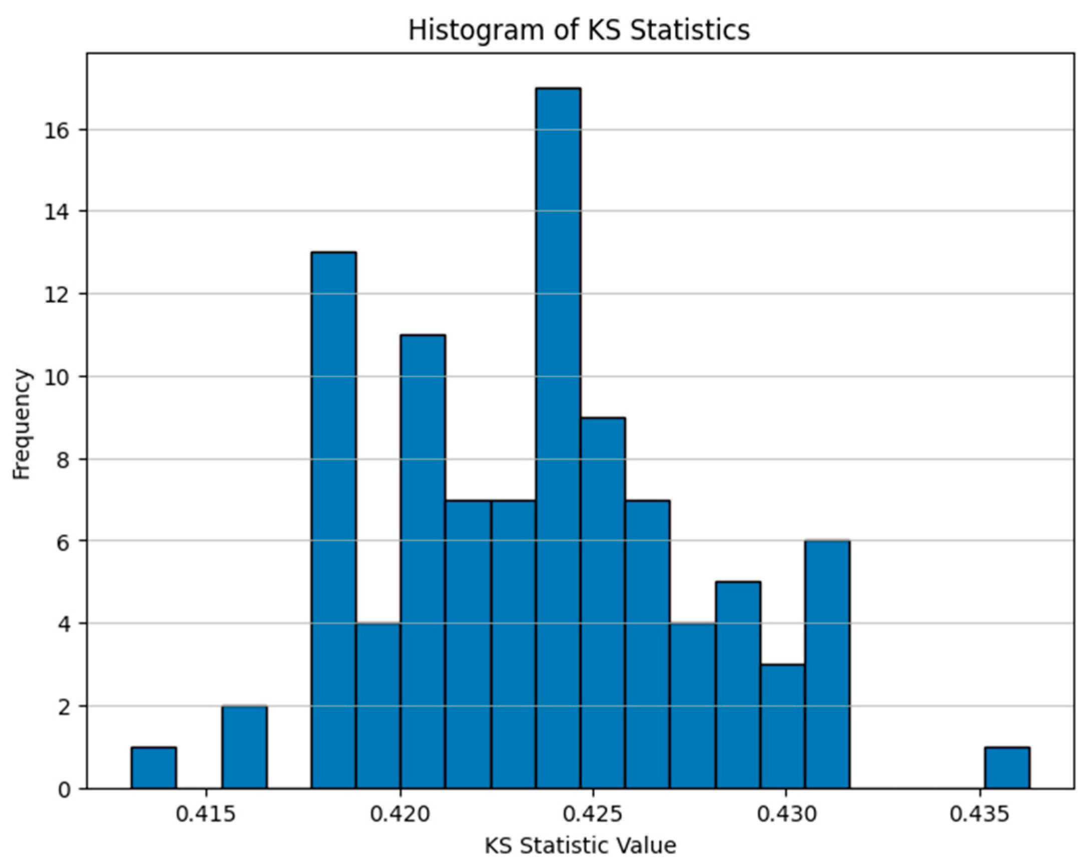
The Kolmogorov–Smirnov (KS) values across the 100 independently trained XGBoost models demonstrate strong and consistent discriminatory performance. As shown in Figure 2, KS values range from 41.31% to 43.63%, with a median of 42.37%. The narrow range indicates that different random seed initializations have minimal impact on model discrimination ability, confirming that all models exhibit comparable predictive strength.

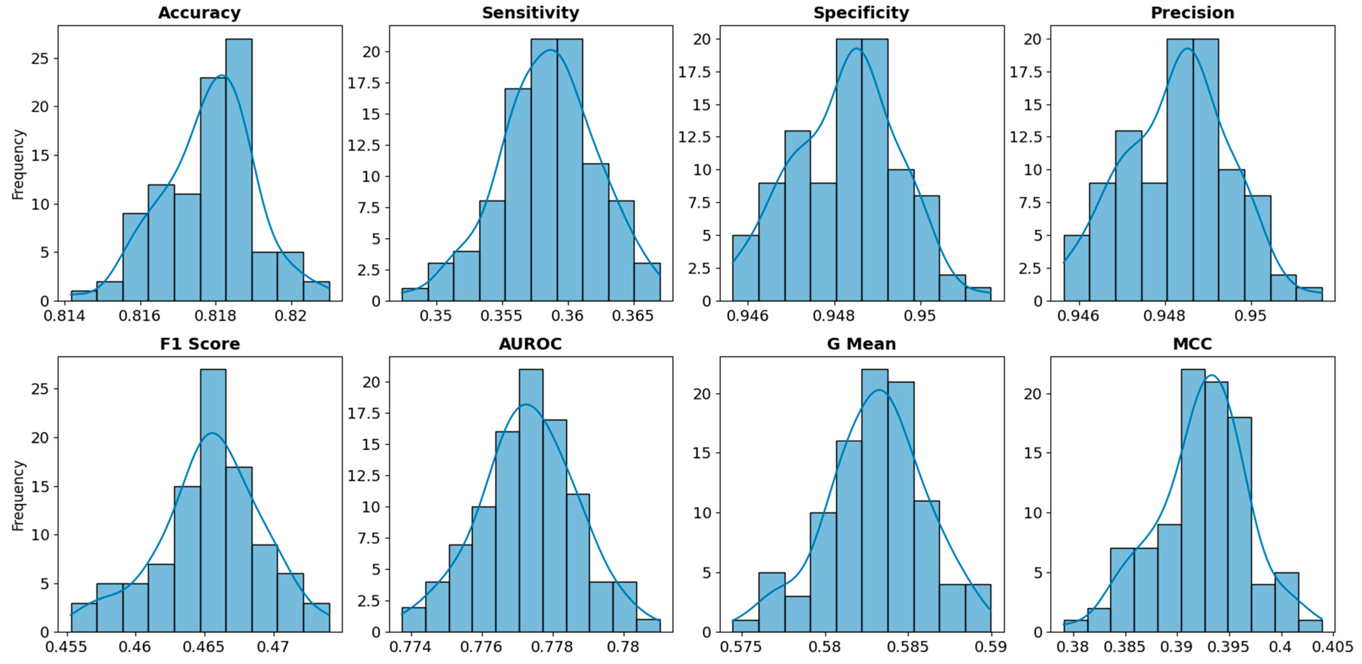
Figure 3 below presents the distribution of confusion matrix derived metrics across the 100 trained XGBoost models, while

Table 3. Confusion Matrix Median and 95% Confidence Interval (CI).

Metric	Median	Lower 95% CI	Upper 95% CI
Accuracy	79.53%	79.25%	79.77%
Sensitivity	53.73%	53.08%	54.26%
Specificity	86.86%	86.68%	87.01%
Precision	86.86%	86.68%	87.01%
F1 Score	53.73%	53.08%	54.26%
AUROC	77.73%	77.46%	78.00%
G Mean	68.32%	67.83%	68.71%
MCC	40.59%	39.76%	41.27%

shows the median values and the corresponding 95% confidence interval and median value for each metric. Similarly, the results show that model performance remains highly consistent across all models, confirming the limited effects of initial seeds randomization. The median accuracy of approximately 79.5% reflects strong predictive capability, comparable to benchmark findings reported in recent study (Bhandary and Ghosh 2025).

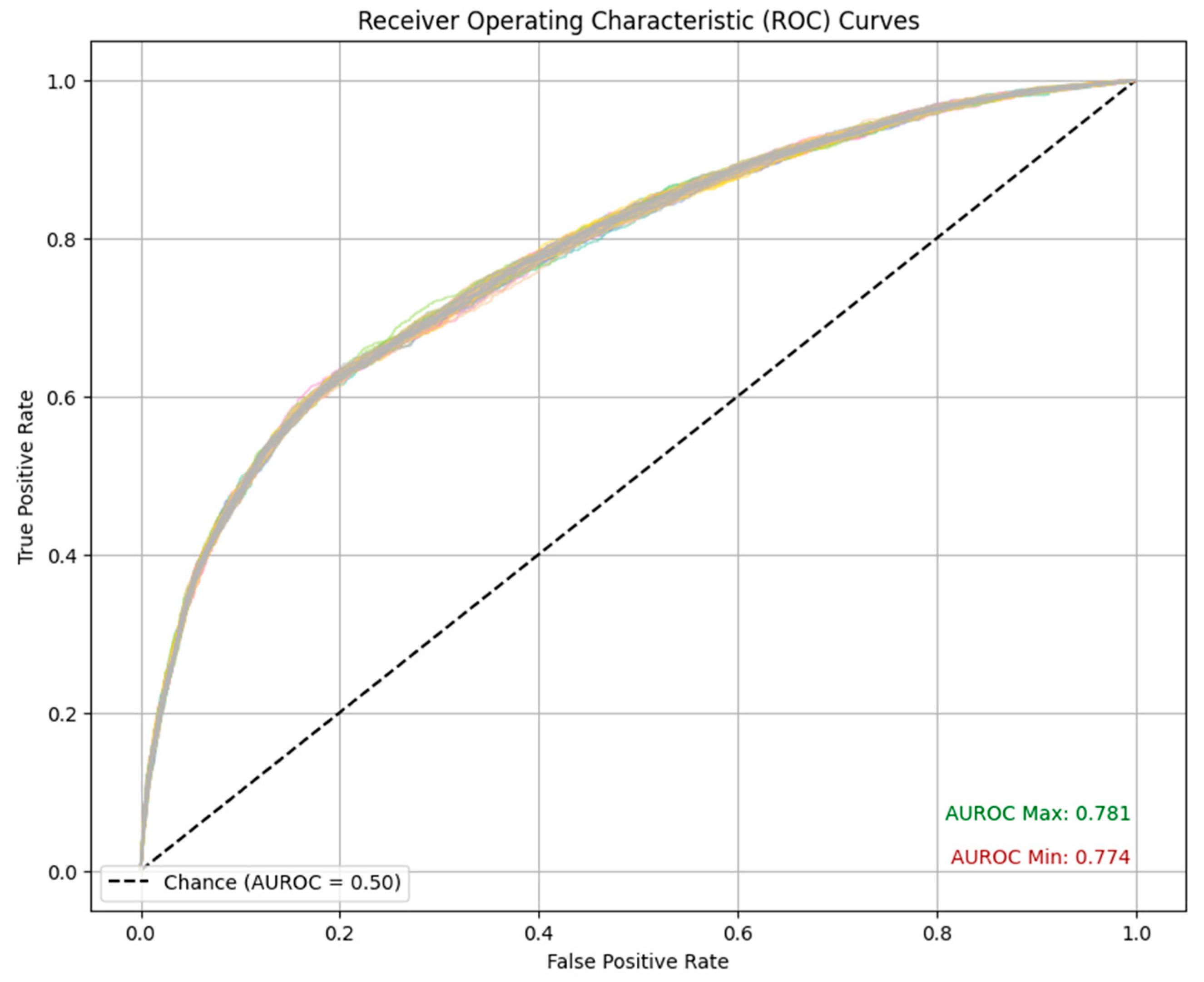
As illustrated in Figure 4, the ROC curves across all models are nearly indistinguishable, with AUROC values narrowly ranging between 0.774 and 0.781. This consistency highlights the stability of the models’ prediction power across different random seed initializations.

4.2. Global SHAP Evaluation

Having examined that all models exhibit consistent predictive performance, we can reasonably attribute any observed variation in SHAPs to differences in seed initialization rather than discrepancies in model accuracy. Hence, this section evaluates the global stability of SHAP-based feature importance across the 100 independently trained models.

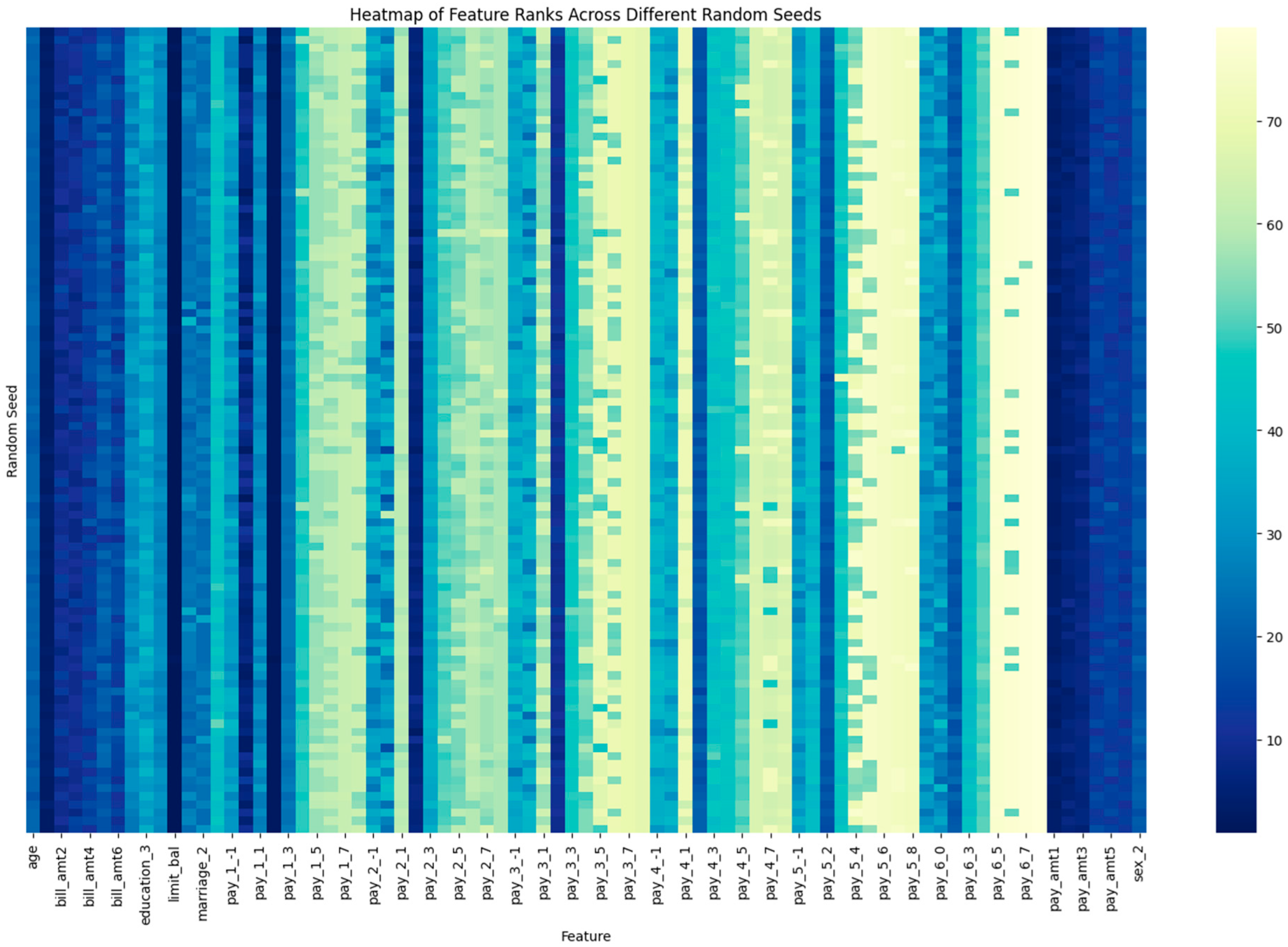
Figure 5 displays the heatmap of SHAP feature ranking across those models. Each cell represents the relative rank of a specific feature (X-axis) within a model (Y-axis), where darker color corresponds to higher feature importance. It reveals that features at the top and bottom of the ranking spectrum exhibit remarkable stability across models with different random seeds. In contrast, features in the middle range of importance show greater variability in the rankings, suggesting that moderate features are more sensitive to model initialization.

To further examine the stability pattern observed in the heatmap, we take a closer look at the features exhibiting the highest and lowest rank consistency across models.

Table 4. List of 5 Variables with highest SHAP mean rank.

Variable	Meaning	Rank	Frequence
Limit_bal	Amount of credit given in NT dollars (includes individual and family/supplementary credit	1	96
		2	4
pay_1_2	Repayment status in September 2005: Payment delay for two months	1	4
		2	93
		3	3
bill_amt1	Amount of bill statement in September 2005 (NT dollar)	3	56
		4	39
		5	5
pay_amt1	Amount of previous payment in September 2005 (NT dollar)	3	29
		4	49
		5	17
		6	3
		7	2
pay_amt2	Amount of previous payment in August 2005 (NT dollar)	4	5
		5	46
		6	25
		7	16
		8	7
		9	1

and

Table 5. List of 5 variables with the lowest SHAP mean rank.

Variable	Meaning	Rank	Frequence
pay_5_7	Repayment status in May 2005: Payment delay for seven months	50	1
		73	85
		75	14
pay_5_6	Repayment status in May 2005: Payment delay for six months	73	1
		74	99
pay_6_5	Repayment status in April 2005: Payment delay for five months	76	81
		77	19
pay_6_7	Repayment status in April 2005: Payment delay for seven months	54	1
		78	99
pay_6_8	Repayment status in April 2005: Payment delay for eight months	79	100

summarize the rank distributions for the five features with the highest and lowest mean SHAP ranks, respectively. For instance, feature limit_bal (the amount of given credit in New Taiwan dollars) ranked first in 96 out of 100 models, and second in the remaining four, demonstrating exceptional stability and dominant importance across all models. Similarly, features with consistently low predictive contributions, such as pay_6_8 (an indicator of eight-month payment delays as of April 2005), appear at the boom of the rankings across all models. These results confirm that both highly predictive and negligible variables maintain strong rank stability across different model initializations.

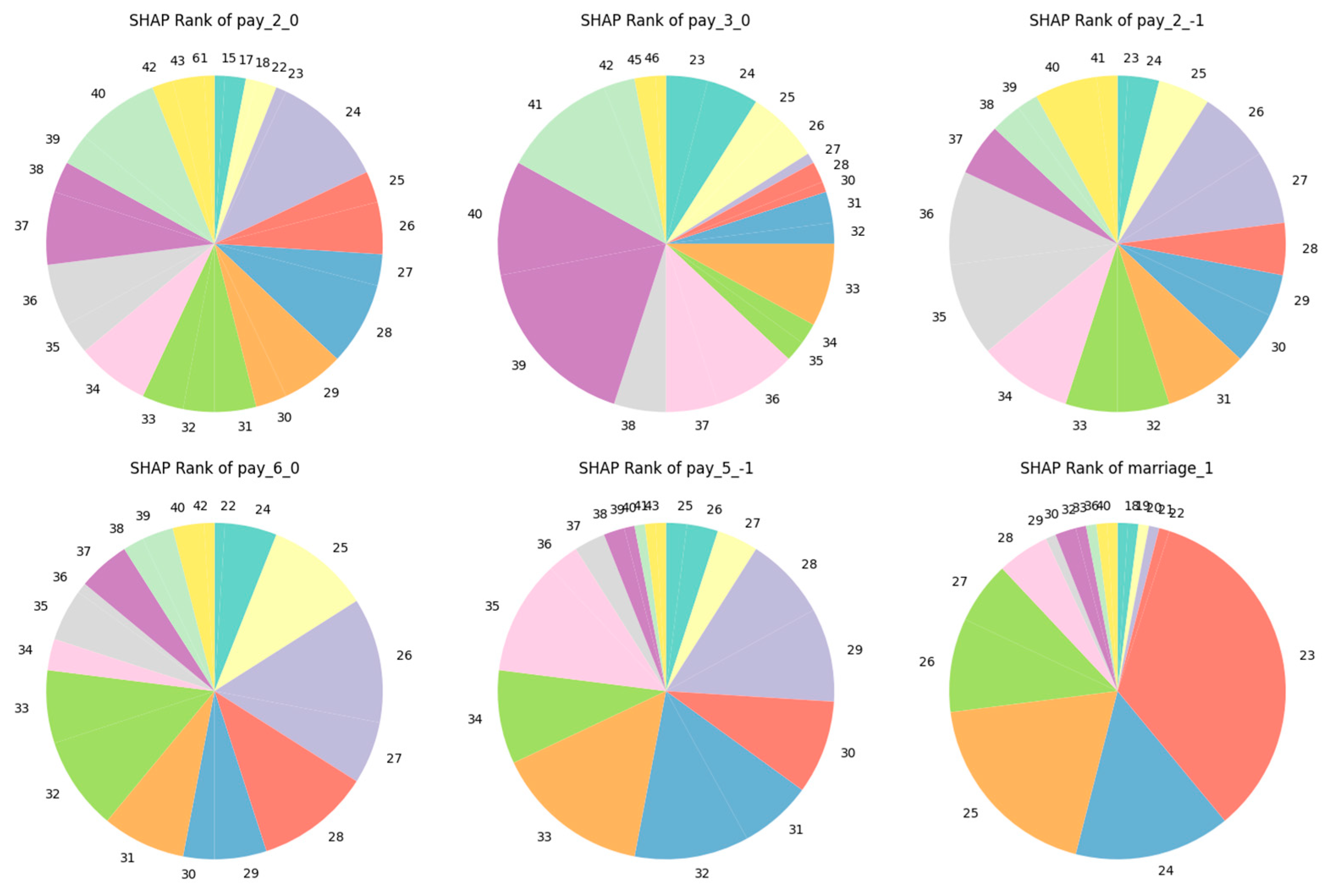
In contrast, features with moderate SHAP importance exhibit noticeably greater variability across models. Figure 6 displays the SHAP rank distributions for the six features with the greatest diversity in ranking among the 100 trained models. Notably, pay_2_0, which indicates the repayment in August 2006 is from the use of revolving credit, shows the highest variability. It has 25 distinct ranking positions, ranging from 15 to 61. The substantial fluctuation suggests that features with moderate predictive strength are more sensitive to random initialization factors, leading to more volatile SHAP-based interpretations.

To assess the ranking stability quantitively, we calculated the Kendall’s W statistic across all features and group of features. The overall Kendall’s W value across all features is 0.98, indicating a very high level of agreement in feature importance rankings. The associated chi-square test yielded a statistic of ${\chi }^2$ = 7626.93 with 78 degrees of freedom and a p-value less than 0.001. The low p-value confirmed that the observed consistency is statistically significant rather than due to chance.

For the top five features listed in Table 4, the Kendall’s W value is 0.93, corresponding to a chi-square statistics of ${\chi }^2$ = 371.94 with 4 degrees of freedom, indicating a high degree of stability in SHAP rankings. In contrast, for the six features shown in Figure 6, the value decreases to 0.34, with ${\chi }^2$ = 167.58 and 5 degrees of freedom, reflecting substantially lower concordance. This difference further supports that features with moderate predictive importance exhibit significant lower SHAP ranking stability compared with the top-ranked features.

5. Discussion and Implications

In this study, we explore how random seed initializations in XGBoost models affect the stability of SHAP-based feature rankings in credit risk modeling via a case study on the Default of Credit Risk dataset. Using 100 independently trained XGBoost classifiers with various random seeds, we observe clear and systematic differences in stability across features of varying importance. Features at both the high and low ends of the importance spectrum remain highly stable, exhibiting limited variation in ranking positions across different models. In contrast, features of moderate importance show considerably higher variability, indicating greater sensitivity to random seed initialization.

This pattern is further supported by Kendall’s W statistics and the corresponding chi-square tests. For the top five important features, Kendall’s W equals 0.93 (χ² = 371.94, degree of freedom = 4), reflecting strong alignment in SHAP rankings across models. Conversely, for the six moderately important features, Kendall’s W decreases sharply to 0.3352 (χ² = 167.58, degree of freedom = 5), highlighting a substantially lower level of concordance. These results collectively demonstrate that SHAP-based ranking stability I closely linked to the underlying feature importance level: dominant and negligible predictors exhibit consistent orderings, whereas mid-importance features account for most of the observed instability under random seed perturbations.

The observed patterns can be explained from a modeling perspective. By the nature of XGBoost algorithm, these dominant features may repeatedly appear in early splits of the decision trees, leading to stable SHAP rankings regardless of the random seed initialization. Similarly, features with very low predictive power contribute minimally to the model and therefore maintain consistently low SHAP rankings across models. In contrast, features of moderate predictive operate in a more competitive zone. A small change in initialization can alter the sequence of feature splits and thus the resulting SHAP attributions.

Our study extends existing research on the robustness of SHAP in credit risk modeling. Previous studies have primarily focused on SHAP stability under class imbalance, showing that the increasing imbalance ratios significantly reduced the consistency of SHAPs (Chen et al. 2024; Ballegeer et al. 2025). To the best of our knowledge, this is the first study to isolate and examine the effect of random seed initialization on SHAP stability. The results reveal that even under a fixed imbalance ratio, random initialization alone can also introduce variation in SHAP feature rankings, especially for features with moderate importance. This research provides novel empirical understanding of SHAP reliability in high-stakes financial applications.

6. Conclusions

While the study provides an empirical evaluation of SHAP stability under different random seed initializations, several limitations should be noted. First, the analysis is based on a case study, where a single public dataset is evaluated based on the XGBoost algorithm only. Although this setting allows for experiment simplicity and reproducibility, the findings may not fully generalize to other credit portfolios or to alternative ML model classes. Future research could extend the analysis to a wider range of datasets with diverse portfolio characteristics (e.g., mortgage, auto, or small-business lending) or to various model architectures (e.g., random forests or neural network). In addition, our evaluation replies on a specific set of assessment, which is to evaluate SHAP stability using models trained with varying random seeds. Other types of robustness tests, such as those examining the effects of data imbalance or alternative sampling schemes, are not explored. These alternative tests may reveal other patterns of SHAP variability that are not captured in the current study. Finally, the study is primarily empirical and does not provide a formal theoretical explanation for the mechanisms underlying SHAP instability. Further analytical studies are needed to establish a more rigorous understanding of the fundamental drivers of SHAP variability.

We also would like to provide some suggestions for both practitioners and regulators in credit risk based on the empirical results. First, model developers and validators should consider SHAP stability when assessing model interpretability. Aggregated SHAP-based importance ranking based on ensemble approach can be considered as a more robust and representative view of feature contributions, reducing the risk of biased interpretation results driven by individual model. In addition, special caution should be taken when using mid-importance features in adverse action reasoning. The high variability in SHAP rankings of those features could lead to inconsistent or misleading explanations for credit decision justify. Before adding them in customer-facing communications or compliance reports, institutions should perform additional test to verify the explanation stability. In general, we want to emphasize the need of explainable AI stability assessment in credit decision models to ensure fairness and reliability.

In summary, this study demonstrates that SHAP-based explanation ranking is affected by random seed initialization, particularly for features of moderate importance. These findings highlight the importance of incorporating stability assessment into feature explanations to ensure consistent and reliable interpretations in credit risk modeling.

References

1. Alonso, Andrés, and Jose Manuel Carbo. 2020. Machine Learning in Credit Risk: Measuring the Dilemma Between Prediction and Supervisory Cost. Banco de Espana Working Paper No. 2032. Available online: https://papers.ssrn.com/sol3/papers.cfm?abstract_id=3724374 (accessed on 3 October 2025).
2. Baesens, Bart, Tony Van Gestel, Stijn Viaene, Maria Stepanova, Johan Suykens, and Jan Vanthienen. 2003. Benchmarking State-of-the-Art Classification Algorithms for Credit Scoring. Journal of the Operational Research Society 54: 627–35. [Google Scholar] [CrossRef]
3. Ballegeer, Matteo, Matthias Bogaert, and Dries F. Benoit. 2025. Evaluating the Stability of Model Explanations in Instance-Dependent Cost-Sensitive Credit Scoring. European Journal of Operational Research 326: 630–40. [Google Scholar] [CrossRef]
4. Bhandary, Rakshith, and Bidyut Kumar Ghosh. 2025. Credit Card Default Prediction: An Empirical Analysis on Predictive Performance Using Statistical and Machine Learning Methods. Journal of Risk and Financial Management 18: 23. [Google Scholar] [CrossRef]
5. Board of Governors of the Federal Reserve System. 2011. Supervisory Guidance on Model Risk Management (SR 11-7); Washington, DC: Federal Reserve and Office of the Comptroller of the Currency. Available online: https://www.federalreserve.gov/supervisionreg/srletters/sr1107.htm (accessed on 16 May 2025).
6. Bolton, Christine. 2009. Logistic Regression and Its Application in Credit Scoring. Available online: https://www.proquest.com/openview/134cf4372fbb2bc5b6f9cbda4c559337/1?pq-origsite=gscholar&cbl=2026366&diss=y (accessed on 10 June 2025).
7. Boser, Bernhard E., Isabelle M. Guyon, and Vladimir N. Vapnik. 1992. A Training Algorithm for Optimal Margin Classifiers. Paper presented at Fifth Annual Workshop on Computational Learning Theory, Pittsburgh, PA, USA, July 27–29; pp. 144–52. [Google Scholar]
8. Breiman, Leo. 2001. Random Forests. Machine Learning 45: 5–32. [Google Scholar] [CrossRef]
9. Bussmann, Niklas, Paolo Giudici, Dimitri Marinelli, and Jochen Papenbrock. 2021. Explainable Machine Learning in Credit Risk Management. Computational Economics 57: 203–16. [Google Scholar] [CrossRef]
10. Castelvecchi, Davide. 2016. Can We Open the Black Box of AI? News Feature. Nature News 538: 20. [Google Scholar] [CrossRef]
11. Chen, Tianqi, and Carlos Guestrin. 2016. Xgboost: A Scalable Tree Boosting System. Paper presented at 22nd Acm Sigkdd International Conference on Knowledge Discovery and Data Mining, San Francisco, CA, USA, August 13–17; pp. 785–94. [Google Scholar]
12. Chen, Yujia, Raffaella Calabrese, and Belen Martin-Barragan. 2024. Interpretable Machine Learning for Imbalanced Credit Scoring Datasets. European Journal of Operational Research 312: 357–72. [Google Scholar] [CrossRef]
13. Consumer Financial Protection Bureau. 2022. Consumer Financial Protection Circular 2022-03: Adverse Action Notification Requirements in Connection with Credit Decisions Based on Complex Algorithms. June. Available online: https://www.govinfo.gov/content/pkg/FR-2022-06-14/pdf/2022-12729.pdf (accessed on 16 May 2025).
14. Consumer Financial Protection Bureau. 2023. The Consumer Credit Card Market Report, 2023; Washington, DC: Consumer Financial Protection Bureau. Available online: https://www.federalregister.gov/documents/2023/11/02/2023-24132/consumer-credit-card-market-report-2023 (accessed on 16 May 2025).
15. Černevičienė, Jurgita, and Audrius Kabašinskas. 2024. Explainable Artificial Intelligence (XAI) in Finance: A Systematic Literature Review. Artificial Intelligence Review 57: 216. [Google Scholar] [CrossRef]
16. Dwivedi, Rudresh, Devam Dave, Het Naik, Smiti Singhal, Rana Omer, Pankesh Patel, Bin Qian, Zhenyu Wen, Tejal Shah, Graham Morgan, and et al. 2023. Explainable AI (XAI): Core Ideas, Techniques, and Solutions. ACM Computing Surveys 55: 1–33. [Google Scholar] [CrossRef]
17. Equal Credit Opportunity Act. 2024. Available online: https://www.ftc.gov/legal-library/browse/statutes/equal-credit-opportunity-act (accessed on 14 July 2025).
18. Fair Credit Reporting Act. 2023. Available online: https://www.ftc.gov/system/files/ftc_gov/pdf/fcra-may2023-508.pdf (accessed on 14 July 2025).
19. Friedman, Jerome H. 2001. Greedy Function Approximation: A Gradient Boosting Machine. Annals of Statistics 29: 1189–232. [Google Scholar] [CrossRef]
20. Géron, Aurélien. 2022. Hands-On Machine Learning with Scikit-Learn, Keras, and TensorFlow. Sebastopol: O’Reilly Media, Inc. [Google Scholar]
21. Gupta, Nikhil. 2025. Explainable AI for Regulatory Compliance in Financial and Healthcare Sectors: A Comprehensive Review. International Journal of Advances in Engineering and Management 7: 489–94. [Google Scholar] [CrossRef]
22. Hand, David J., and William E. Henley. 1997. Statistical Classification Methods in Consumer Credit Scoring: A Review. Journal of the Royal Statistical Society: Series A (Statistics in Society) 160: 523–41. [Google Scholar] [CrossRef]
23. Hlongwane, Rivalani, Kutlwano Ramabao, and Wilson Mongwe. 2024. A Novel Framework for Enhancing Transparency in Credit Scoring: Leveraging Shapley Values for Interpretable Credit Scorecards. PLoS ONE 19: e0308718. [Google Scholar] [CrossRef]
24. International Financial Reportings Standard 9 Financial Instruments. 2019. Available online: https://www.ifrs.org/content/dam/ifrs/publications/pdf-standards/english/2022/issued/part-a/ifrs-9-financial-instruments.pdf?bypass=on (accessed on 14 July 2025).
25. Kendall, Maurice G., and B. Babington Smith. 1939. The Problem of m Rankings. The Annals of Mathematical Statistics 10: 275–87. [Google Scholar] [CrossRef]
26. Kuhn, Max, and Kjell Johnson. 2013. Applied Predictive Modeling. Berlin and Heidelberg: Springer. [Google Scholar]
27. Lessmann, Stefan, Bart Baesens, Hsin-Vonn Seow, and Lyn C. Thomas. 2015. Benchmarking State-of-the-Art Classification Algorithms for Credit Scoring: An Update of Research. European Journal of Operational Research 247: 124–36. [Google Scholar] [CrossRef]
28. Liu, Mingxuan, Yilin Ning, Han Yuan, Marcus Eng Hock Ong, and Nan Liu. 2022. Balanced Background and Explanation Data Are Needed in Explaining Deep Learning Models with SHAP: An Empirical Study on Clinical Decision Making. arXiv arXiv:2206.04050. [Google Scholar] [CrossRef]
29. Lundberg, Scott M., and Su-In Lee. 2017. A Unified Approach to Interpreting Model Predictions. Advances in Neural Information Processing Systems 30: 4768–77. [Google Scholar] [CrossRef]
30. Misheva, Branka Hadji, Joerg Osterrieder, Ali Hirsa, Onkar Kulkarni, and Stephen Fung Lin. 2021. Explainable AI in Credit Risk Management. arXiv arXiv:2103.00949. [Google Scholar] [CrossRef]
31. Molnar, Christoph. 2019. Interpretable Machine Learning. Available online: https://www.google.com/books?hl=en&lr=&id=jBm3DwAAQBAJ&oi=fnd&pg=PP1&dq=Molnar,+Christoph.+2019.+Interpretable+Machine+Learning.&ots=EhxTUnJEQ1&sig=d3rIDzBa22-dd92ObB6D1LqI340 (accessed on 15 July 2025).
32. Montevechi, André Aoun, Rafael De Carvalho Miranda, André Luiz Medeiros, and José Arnaldo Barra Montevechi. 2024. Advancing Credit Risk Modelling with Machine Learning: A Comprehensive Review of the State-of-the-Art. Engineering Applications of Artificial Intelligence 137: 109082. [Google Scholar] [CrossRef]
33. Mvula Chijoriga, Marcellina. 2011. Application of Multiple Discriminant Analysis (MDA) as a Credit Scoring and Risk Assessment Model. International Journal of Emerging Markets 6: 132–47. [Google Scholar] [CrossRef]
34. Mylonakis, John, and George Diacogiannis. 2010. Evaluating the Likelihood of Using Linear Discriminant Analysis as A Commercial Bank Card Owners Credit Scoring Model. International Business Research 3: 9. [Google Scholar] [CrossRef]
35. Nielsen, Didrik. 2016. Tree Boosting with Xgboost-Why Does Xgboost Win” Every” Machine Learning Competition? Master’s thesis, NTNU, Trondheim, Norway. [Google Scholar]
36. Pérez-Cruz, Fernando, Jermy Prenio, Fernando Restoy, and Jeffery Yong. 2025. Managing Explanations: How Regulators Can Address AI Explainability. Available online: https://www.fiduciacorp.com/s/BIS-Mangaing-AI-Expectations.pdf (accessed on 15 July 2025).
37. Ribeiro, Marco Tulio, Sameer Singh, and Carlos Guestrin. 2016. ‘Why Should I Trust You?’: Explaining the Predictions of Any Classifier. arXiv arXiv:1602.04938. [Google Scholar] [CrossRef]
38. Rudin, Cynthia. 2019. Stop Explaining Black Box Machine Learning Models for High Stakes Decisions and Use Interpretable Models Instead. Nature Machine Intelligence 1: 206–15. [Google Scholar] [CrossRef]
39. Scott Lundberg. 2025. SHAP (SHapley Additive exPlanations) Documentation. Available online: https://shap.readthedocs.io/en/latest/index.html (accessed on 20 April 2025).
40. Shukla, Deepa. 2024. A Survey of Machine Learning Algorithms in Credit Risk Assessment. Journal of Electrical Systems 20: 6290–97. [Google Scholar] [CrossRef]
41. Siddiqi, Naeem. 2012. Credit Risk Scorecards: Developing and Implementing Intelligent Credit Scoring. Hoboken: John Wiley & Sons. [Google Scholar]
42. Suhadolnik, Nicolas, Jo Ueyama, and Sergio Da Silva. 2023. Machine Learning for Enhanced Credit Risk Assessment: An Empirical Approach. Journal of Risk and Financial Management 16: 496. [Google Scholar] [CrossRef]
43. Supervision, Banking. 2011. Basel Committee on Banking Supervision. Principles for Sound Liquidity Risk Management and Supervision (September 2008). Available online: https://www.academia.edu/download/45696423/bcbs213.pdf (accessed on 12 June 2025).
44. Thomas, Lyn C., David B. Edelman, and Jonathan N. Crook. 2002. Credit Scoring and Its Applications. Philadelphia: SIAM. [Google Scholar]
45. Weber, Patrick, K. Valerie Carl, and Oliver Hinz. 2024. Applications of Explainable Artificial Intelligence in Finance—Traditional statistical approaches Systematic Review of Finance, Information Systems, and Computer Science Literature. Management Review Quarterly 74: 867–907. [Google Scholar] [CrossRef]
46. Xgboost 3.1.1. 2025. Available online: https://xgboost.readthedocs.io/en/stable/tutorials/feature_interaction_constraint.html?utm_source=chatgpt.com (accessed on 5 April 2025).
47. Yeh, I-Cheng. 2009. Default of Credit Card Clients. Irvine: UCI Machine Learning Repository. [Google Scholar] [CrossRef]
48. Yeo, Wei Jie, Wihan Van Der Heever, Rui Mao, Erik Cambria, Ranjan Satapathy, and Gianmarco Mengaldo. 2025. A Comprehensive Review on Financial Explainable AI. Artificial Intelligence Review 58: 189. [Google Scholar] [CrossRef]
Figure 1. Experiment Design Flowchart.
Risks 13 00238 g001
Figure 2. KS Performance.
Risks 13 00238 g002
Figure 3. Confusion Metric Distribution Plots.
Risks 13 00238 g003
Figure 4. ROC Curve.
Risks 13 00238 g004
Figure 5. Heatmap of SHAP rank for each variable among models.
Risks 13 00238 g005
Figure 6. Unique SHAP Rank Counts of variables.
Risks 13 00238 g006