Article

Volatility Spillovers and Market Decoupling: Evidence from BRICS and China’s Green Sector

by
Darko B. Vuković
1,2,*,
Dmitrii Leonidovich Fefelov
1,
Michael Frömmel
3 and
Elena Moiseevna Rogova
1
1
Research Center for Market Efficiency and Applied Finance, Graduate School of Management, St. Petersburg State University, 1-3 Volkhovsky Pereulok, 199004 St. Petersburg, Russia
2
Geographical Institute “Jovan Cvijic” SASA, Djure Jaksica 9, 11000 Belgrade, Serbia
3
Department of Economics, Ghent University, Sint-Pietersplein 5, 9000 Gent, Belgium
*
Author to whom correspondence should be addressed.
Risks 2025, 13(11), 222; https://doi.org/10.3390/risks13110222
Submission received: 19 September 2025 / Revised: 14 October 2025 / Accepted: 20 October 2025 / Published: 6 November 2025

Abstract

The global economic importance of green tech is rising. Yet the role of the green financial sector in the propagation of volatility is still unclear. Although the existing literature often characterizes green assets as stable, the new risks, particularly US–China trade tensions that target the green sector directly, may uncover potential vulnerabilities. As China’s green sector has attained global leadership, its interconnections with other major economies require a closer examination, especially within the BRICS block. Applying the Bayesian VAR with Minnesota Ridge prior and a TVP-VAR model-based connectedness approach on a dataset of 1880 observations spanning from 2016 to 2025, we identified that volatility in China’s green sector peaked during the COVID-19 pandemic and resurged in early 2025 amid trade tensions. Uniquely, this study also finds that, despite the intensification of political and economic relations between BRICS members, the interconnectedness of their financial markets has been weakening, suggesting their long-term decoupling and regionalization. From 2016 to 2024, green indices remained historically peripheral, with limited, stable ties to the Nasdaq and SSE. In 2025, short shock-driven transmitter episodes have emerged and indicate an incipient integration rather than a permanent regime change.

1. Introduction

The growing environmental concerns over the last decade have led to a significant surge of investments prioritizing sustainable development (Chițimiea et al. 2021), with a particular focus on its green component (OECD 2024). This trend is supported by the view that green innovative industries, such as clean and renewable energy, electric vehicles (EVs), batteries, etc., are essential for addressing the global challenges outlined in the UN’s sustainable development goals (SDGs) (The United Nations 2015). Since the adoption of the 17 SDGs in 2015 and a number of global agreements to promote a more sustainable and equitable future, green investments have moved beyond a niche interest to become an important element of risk-management and investment strategies. According to BloombergNEF, the global investment in low-carbon energy reached USD 2.1 trillion, highlighting the scale and relevance of green assets in financial markets. The process demonstrates the relevance of green assets for investors. Green assets typically include green equities, bonds, loans, and securitized instruments like asset-backed securities, all aimed at financing environmentally beneficial purposes (Ding and Liu 2023).
Investor interest in sustainable development grows under tighter rules and vocal stakeholders. In China, policy sets clear targets for a green transition across industry, services, and finance (Yue and Nedopil 2025). Ministries set goals, regulators craft legal standards, and fiscal tools steer capital through incentives (Yue and Nedopil 2025). Firms scale up. This mixture of policies and market incentives led China to become one of the leaders in the production of renewable energies, batteries, electric vehicles, and other niches that represent the green sector (Chan 2025). Rising volumes cut unit costs, so Chinese products compete in terms of price in global markets. The numbers frame the shift: in 2024, the green technology sector topped 10 percent of the GDP, with sales and investment near USD 1.9 trillion (Myllyvirta et al. 2025). Finance feels the change, as investor preferences reshape risk premiums and their term structures, which brings green assets to the center of current research (Siddique et al. 2024). Cross-market links add another layer, since volatility spillovers transmit news and policy shocks across assets and regions (Mensi et al. 2021). Researchers test models that price these links and track trend breaks.
The financial literature often describes green investments as relatively stable and less risky than traditional assets, with some studies suggesting that they may even outperform in returns and volatility (Liu et al. 2023; Siddique et al. 2024). However, these assets are not invulnerable. Their volatility can be influenced by money market conditions, climate change risks, and environmental policies (Wang et al. 2024; Ha 2024). Recently, geopolitical tensions between major economies like the USA and China have introduced significant new uncertainties. Export controls on critical minerals and technology transfer restrictions are disrupting global supply chains (Handley et al. 2025), while shifts in climate policy and trade barriers are affecting the demand for green technologies (Dev 2025). These frictions have been linked to a wave of bankruptcies among Chinese solar and electric vehicle producers (Reuters 2025). Even though China’s direct exports of green innovations to the USA are limited (Myllyvirta et al. 2025), the impact is pronounced for emerging markets. BRICS nations like India and South Africa, which consume cheap Chinese EVs (Global Times 2024), and Brazil, a key lithium supplier, which is an important component for renewable batteries (Araújo 2025), now perceive trade tensions as a costly risk to their sustainable transformation and participation in global value chains.
Past recovery programs, including post-pandemic stimulus, lifted the green sector (World Economic Forum 2021). Geopolitically driven crises and trade restrictions now strain it, which sets the first objective of this study: to measure and test time-varying volatility spillovers in the green financial sector under trade wars. Prior research, such as that of Lundgren et al. (2018), focuses on developed markets, and evidence for emerging economies remains thin. The second objective examines bilateral and multilateral spillovers between China’s green indices and emerging market stock markets, with global benchmarks included to isolate external influence. Our study analyzes the following: Do China’s green indices act as net transmitters or net receivers relative to BRICS and a global benchmark on average?
To narrow our focus on emerging economies, our study utilizes data from the BRICS nations. These countries have deep economic ties with China, a leading supplier of green technologies and a major importer of raw materials (Myllyvirta et al. 2025; Global Times 2024), creating channels for financial shock transmission (Bhuyan et al. 2016).
We use daily time series with a ΔPrice and returns system for China’s green sector and BRICS equity markets, covering SSE Sustainable Industry and New Energy Vehicles for China, and the JSE, Bovespa, IMOEX, SSE Composite, and Nifty 50. The study estimates connectedness through a Bayesian vector autoregression and a time-varying parameter VAR to measure total interconnectedness, the direction and size of spillovers, and net as well as net pairwise effects (Antonakakis et al. 2019). A LASSO stage reduces redundant variables and sharpens the model selection. The contribution rests in three elements. First, the analysis moves the spillover debate from developed markets to a BRICS setting that centers on China’s green indices, where prior evidence remains thin (Lundgren et al. 2018). Second, the design combines BVAR and TVP VAR for a common daily sample to compare static network features with their time-varying counterparts, which addresses regime shifts tied to policy and trade frictions that recent reports link to green sector stress and recovery cycles (World Economic Forum 2021). Third, the LASSO filter separates thematic green transmission from broad market co-movement and yields a ranked map of bilateral and net effects that standard connectedness studies often leave implicit (Fefelov et al. 2025). The paper proceeds with the theoretical foundations, methodology, findings, and discussion.

2. Theoretical Foundations

2.1. The Mechanisms of Green Investments

Green investment dynamics follow how markets set prices. In the efficient view, prices absorb the available information (Fama 1970). Positive news tends to move prices faster than negative news, which often unwinds more slowly (Busse and Green 2002). Gaps in information and frictions tied to institutions create mispricing and room for arbitrage (Lin and Tan 2023). Securities respond to distinct mixes of internal and external drivers, and green assets carry a different mix from legacy sectors.
Policy and sentiment sit at the center of that mix. In China, public demand and ambitious national goals channel capital toward green industries, push traditional producers toward cleaner processes, and broaden the product set that can attract funds and meet rules (Shen et al. 2020). Banks issue bonds to finance green infrastructure, which signals investable pipelines and draws investors (Lin 2023). Prices respond in step with scale: the New Energy Vehicle index rose about fourfold from 2016 to 2022 (Wind Terminal 2025). Firms publish sustainability reports to inform markets, yet evidence on returns and risk remains mixed for green equities. Some studies find weak or negative links or short-lived effects, and greenwashing or data gaps can dull the signal of disclosure (Ding et al. 2024; Alsahlawi et al. 2021).
While Fama (1970) posits price efficiency, green asset volatility is often governed by regulatory and sentiment-driven factors. Risk pricing also tracks climate exposure and investor preferences. Some investors target sustainability outcomes as part of hedging, which can lift prices in upswings and set up sharp pullbacks when sentiment turns (Papathanasiou and Koutsokostas 2024). Rising climate risk raises green energy prices and reduces their volatility; links with oil weaken, and green assets hedge oil risk better than gold (Yuan et al. 2023). Innovation news and digital sentiment add force, as markets reward environmental R&D announcements and react to internet mood in the post-COVID period (Gao et al. 2022). News does not fully account for spillovers, so volatility work needs models that capture market links and time variation to track these shifts (Jiang et al. 2012).

2.2. Turbulence, Spillovers, and Global Interconnectedness

Crisis periods amplify volatility in green investments. System-wide shocks tighten links among green assets; in China, COVID-19 raised connectedness across green stocks, bonds, and carbon markets (Ye et al. 2025). Large shocks lift volatility and carry it across markets, and the type of crisis shapes whether spillovers intensify or ease (Vukovic et al. 2019). During pandemics, short horizon spillovers dominate, with green bonds acting as net transmitters in the short run and net recipients in the long run (Mensi et al. 2023). History also shows regime shifts: after 2008, asymmetries in spillovers fell in total and directional terms, and negative return shocks contributed more to volatility spillovers than positive ones (Baruník et al. 2016). Following Baruník et al. (2016), we examine asymmetries in spillovers, focusing on green assets as potential volatility receivers.
Roles within the green complex remain unclear and need verification. The shock origin matters as well: the US market often leads volatility; shocks spread outward, and bad news spillovers can rebound to US equities (Zhou et al. 2012). The literature diverges on propagation paths, with evidence that oil and gas initiate spillovers that then reach other sectors (He et al. 2025), and other work showing that, under high volatility, green firms can transmit risk (Zhou and Wang 2024). Green equities have sustained relatively well during COVID-19 and periods of geopolitical tension (Mensi et al. 2023; Yiming et al. 2024; Ha 2024).

3. Methodology

3.1. Materials and Methods

3.1.1. Markets and Variables (ΔPrice and Returns)

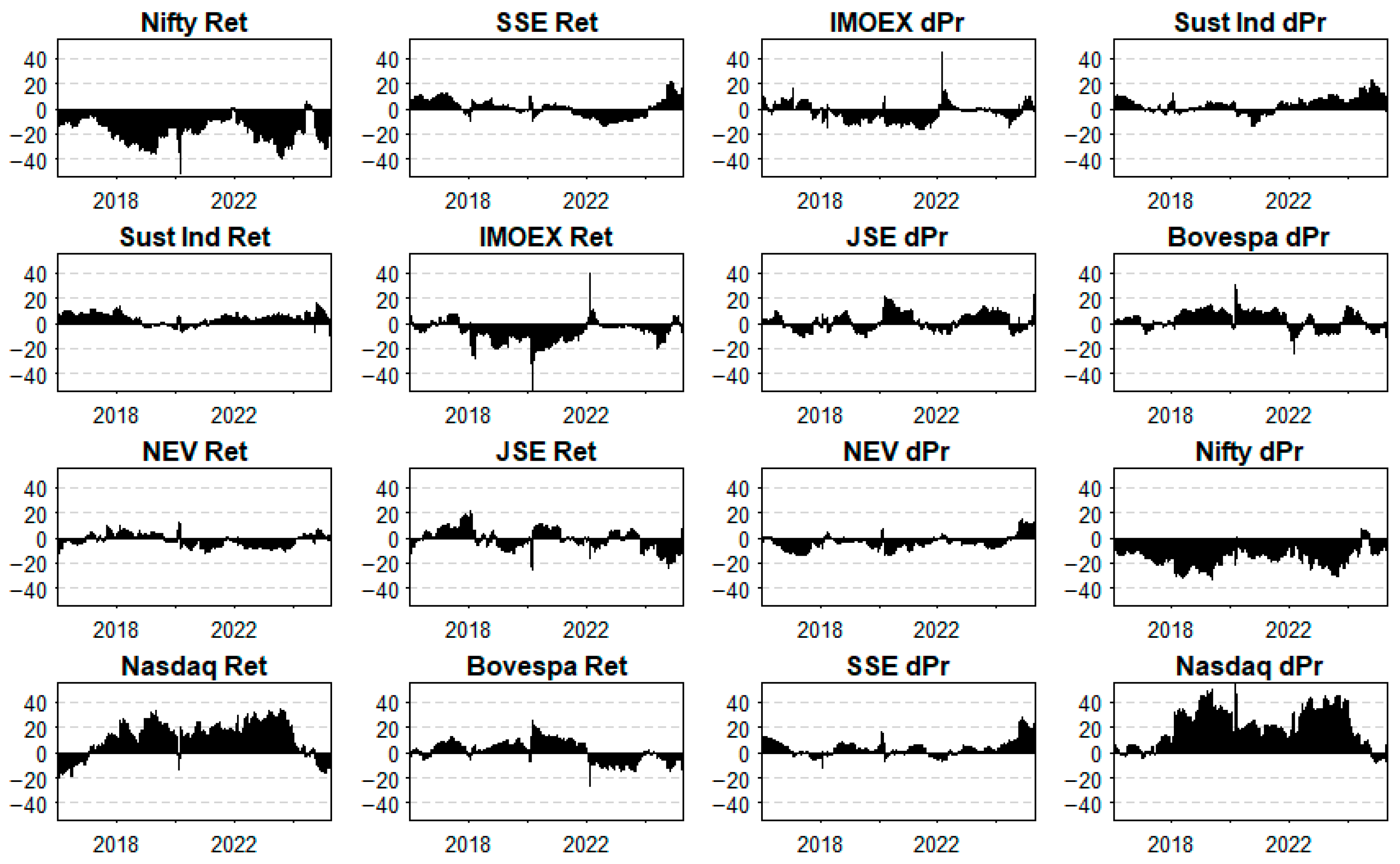
To study spillovers between green and traditional stock markets, the sample covers eight markets or indices, with two variables per asset: ΔPrice (first differences in price levels) and returns. The green segment includes three Chinese indices: SSE Sustainable Industry (Sust Ind), New Energy Vehicles (NEV), and New Energy. We do not include New Energy due to its high correlation with NEV. The BRICS set includes IMOEX for Russia, Nifty 50 for India, Bovespa for Brazil, JSE for South Africa, and the SSE Composite for China. We add the Nasdaq Composite as the global proxy. The Nasdaq skews toward technology and high growth, and investor sentiment toward green firms reacts to innovation signals. Evidence also shows strong links between the Nasdaq and the S&P 500, where using one or the other does not change results in a material way (Galbraith and Zernov 2009).
Table 1 lists the variables used in the model. For plotting clarity, the table reports abridged variable names and their descriptions. The dataset spans May 2016 to April 2025, which covers the major events of the last decade. Sources: Wind Terminal and Investing.com (Wind Terminal 2025; Investing.com 2025).

3.1.2. Summary Statistics and Stationarity Checks

To align the data with BVAR and TVP VAR requirements, we run diagnostics for stationarity and check for misspecification from heteroscedasticity and non-normality. VAR frameworks tolerate some deviations, yet clear diagnostics help set priors and ground the interpretation of results. We begin with stationarity and apply the Kwiatkowski–Phillips–Schmidt–Shin test, which evaluates stationarity around a deterministic trend, a common feature of financial series (see Table A1 in Appendix A).
The tests show unit roots in all price series and stationarity in all return series. After log-differencing, prices become trend stationary, denoted as ΔPrice. This pattern supports the ΔPrice + returns specification used in the study. We then report summary statistics for returns and stationary prices across the eight indices in Table 2.
Returns show a negative skewness: crashes occur more often or with larger magnitudes than rallies. Kurtosis is high across series, which signals fat tails, recurrent stress, and non-normality. IMOEX posts the highest kurtosis, consistent with Russia’s geopolitical instability. Nifty 50 shows a marked tilt toward sharp declines, whereas JSE and SSE look steadier. Bovespa and Nasdaq display wide swings and elevated volatility. Within the green set, China’s Sustainability and NEV indices have the lowest kurtosis; NEV is the only series with a positive skewness, so large moves skew toward gains. These distributional features motivate BVAR and TVP VAR specifications with priors and error terms that account for fat tails and asymmetry.

3.1.3. BVAR Model with Minnesota Ridge Prior

Research on volatility spillovers centers on several strands. Vector autoregression leads the field: Yilmaz (2010) uses a VAR framework to gauge contagion and interdependence across East Asian equities, and Diebold and Yilmaz (2012) formalize total and directional connectedness measures that roll through time. This stream now includes variants such as Bayesian and time-varying parameter setups that address parameter drift and regime shifts, and that identify net transmitters and receivers in a system (Vukovic et al. 2017).
A second strand relies on GARCH models to track second moment dynamics. Multivariate designs capture volatility transmission and time-varying correlations, which show how shocks pass across assets (McMillan and Speight 2010). A third strand uses wavelet methods to separate spillovers by investment horizon, distinguishing short, medium, and long horizons within one dataset (Khalfaoui et al. 2015).
We use a two-step design that links static and time-varying measures of connectedness. First, we implement the Diebold and Yilmaz framework on a stationary VAR(1). The system includes 16 series across 8 markets, with ΔPrice and returns for each. The moving average representation of infinite order yields generalized impulse response functions that do not depend on variable ordering. From these responses, we compute a generalized forecast error variance decomposition at a 10-day horizon and normalize it to a shares matrix. We aggregate off-diagonal shares to form the Total Connectedness Index and the directional indices TO, FROM, and NET for each series. To control overfitting, we place a Bayesian Minnesota prior on the VAR coefficients, and we use bootstrap procedures to form confidence intervals for the impulse responses and for structural breaks in the connectedness paths.
Next, we turn to a time-varying parameter, VAR, to capture evolution in the links without rolling windows. All coefficient matrices, B m ( t ) , change over time, and we derive time, t connectedness, directly from these coefficients. To test the stability of the dynamic links, we add a LASSO specification with an L1 penalty that selects informative predictors and limits multicollinearity, which improves precision and interpretation. As in the Bayesian VAR step, we run the TVP VAR on series that the KPSS tests classify as stationary. Formal expressions appear in Appendix A (Expressions (A1)–(A11)).

4. Results

4.1. Dynamic Interconnectedness Based on BVAR with Minnesota Ridge Prior

We implement a BVAR model on the stationary ΔPrice + returns system. Then, we conduct tests to assess the robustness of the model (Table 3).
Residual diagnostics, Ljung–Box, ARCH-M (lags 1, 5, 10), and distributional tests (Jarque–Bera) reflect the familiar features of daily financial data: conditional heteroskedasticity and non-Gaussian tails. Accordingly, inference in the study relies on GFEVD-based measures (Figure 1) and bootstrap procedures to construct TCI rather than strict normality assumptions.
The GFEVD matrix shows the portion of a variable’s own forecast error variance explained by shocks originating from every other variable in the system. The most isolated variable is the IMOEX return compared to the others, with 0.423 of variance explained by itself. IMOEX ΔPrice ranks second here. IMOEX’s isolation in FEVD suggests regional risk decoupling post-2022 sanctions. However, geographically Chinese markets seem to be the most isolated, as the percentage of FEVD explained by markets from other countries is close to zero. The Nasdaq, JSE, and Bovespa seem particularly to be the main volatility transmitters.
We assess system-wide connectedness with the Total Connectedness Index (TCI; Figure 2) and the NET, TO, and FROM measures (Table A2, Appendix A). We identify variance breaks and segments with a Minnesota Ridge prior set at gamma 0.1; Table A3 reports the predictive accuracy across a grid of gamma values. Over the full sample, TCI follows a declining path. A modest dip appears in 2017, then the index stabilizes near 68 percent in 2018. A large shock in 2020 interrupts this path, and smaller shocks arise again in 2017 and 2025. TCI spans 62.5 percent on 18 September 2023 to 81.4 percent on 15 May 2020, with a mean of 68.68 percent, which indicates a high level of cross-market linkage. The system reacts strongly to the economic and policy uncertainty around COVID-19 in 2020. After that break, TCI resumes a downward drift, with a rebound in April 2025 to 66.1 percent from the 2023 trough.

4.2. Variance Breakpoint and Impulse Response Function Analysis

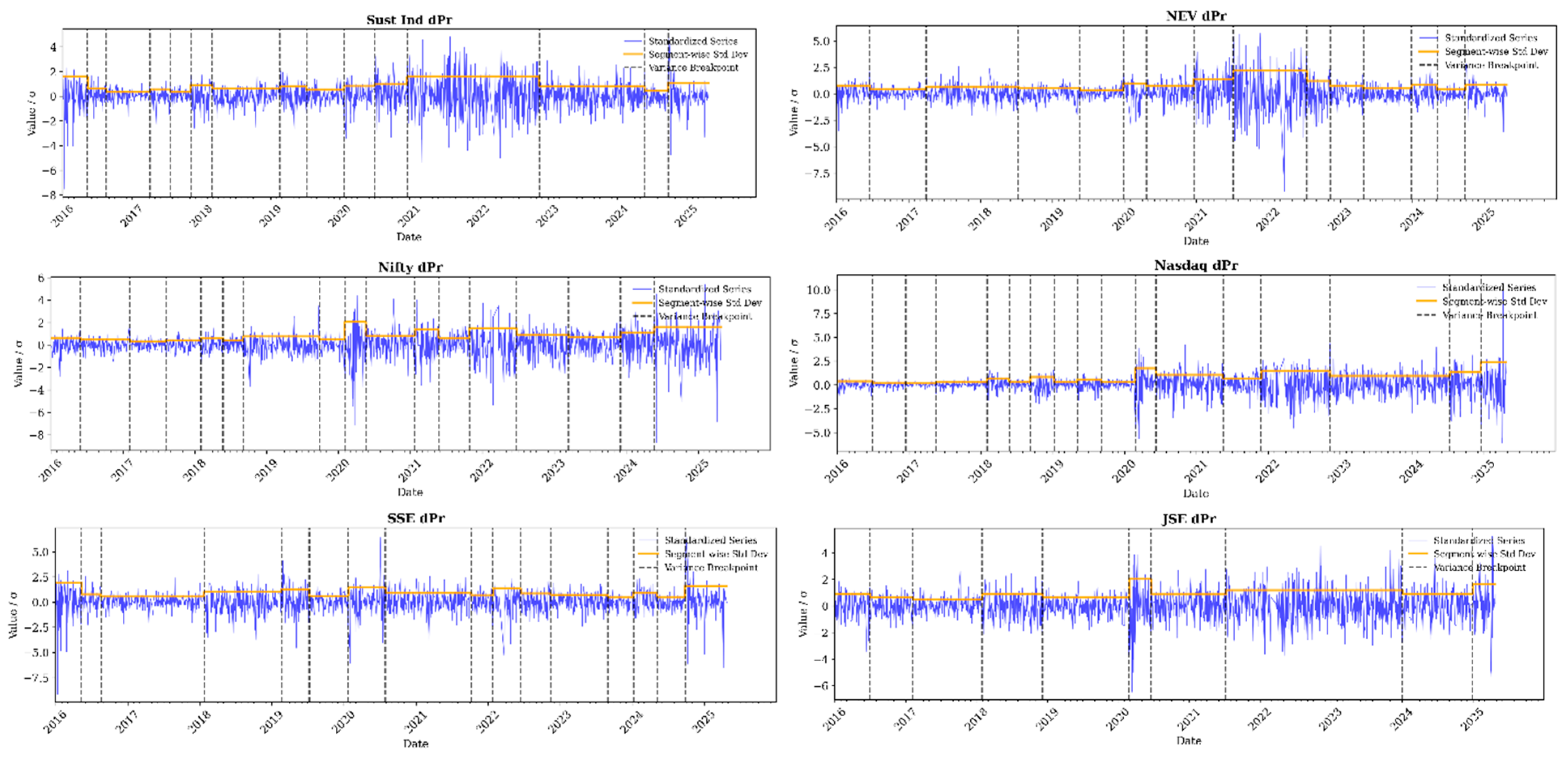
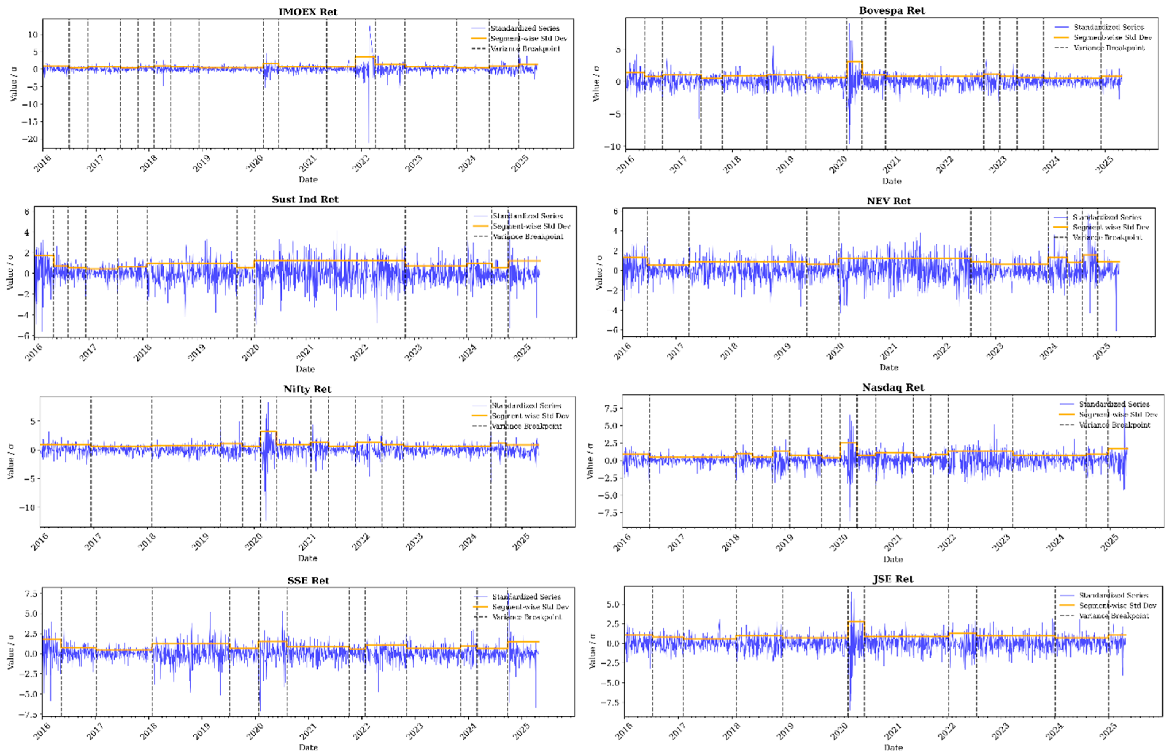
The analysis of variance breakpoints within individual indices shows that volatility patterns are influenced by different events for each market’s prices and returns (Figure 3 and Figure 4, where the blue line depicts standardized series, orange line—segment-wise standard deviation and dashed line—variance breakpoints), with pandemics being the most significant ones, affecting each index. Generally, the NEV indices exhibited a pronounced period of high volatility beginning in early 2019, which persisted through 2021. A major structural breakpoint in 2022 indicates a subsequent steady shift to a lower volatility regime, suggesting a maturation of the sector. Another visible volatility outburst occurred in early 2025 when NEV became the volatility recipient. Sustainable Industry indices demonstrated similar volatility patterns, though with a lesser magnitude. The returns of SSE show stable, low-volatility regimes within the period from 2016 to mid-2018 when the first clear breakpoint occurred, which is possibly tied to geopolitical tensions, such as the US–China trade war and synchronized COVID-19 shocks that caused extreme volatility across all markets later. Unlike the JSE, Nasdaq, and Nifty, SSE’s volatility has reverted to a lower level than the 2018–2020 period, suggesting a decoupling from the higher global volatility.
Nifty stays in a relatively calm, low-volatility state from 2016 to 2020; then, shocks from the pandemic break that pattern. The returns settle from the extreme peaks after 2020, yet ΔPrice records sharp spikes in 2024 and 2025. IMOEX tracks SSE in broad form, yet the 2022 shock hits far harder than in any other market in the sample. The following regime shows extreme volatility and a clear isolation from global finance. JSE holds a medium-to-high volatility state across the full sample, consistent with structural pressures and political uncertainty in South Africa.
Bovespa starts with relatively high volatility in early 2016 (returns), then shifts to a subdued regime through 2017 to 2019. A sharp variance break arrives at the turn of 2020, which matches the COVID-19 shock and the global dollar squeeze. The next regime stays higher, with bursts tied to the commodity rebound, domestic policy, and election headlines in 2021 to 2022. The Nasdaq shows a long stretch of low and falling volatility from 2016 to 2020, supported by tech strength and low rates. The pandemic triggers a clear break. After 2020, volatility settles at a level well above the pre-pandemic period and aligns with the new macro setting.
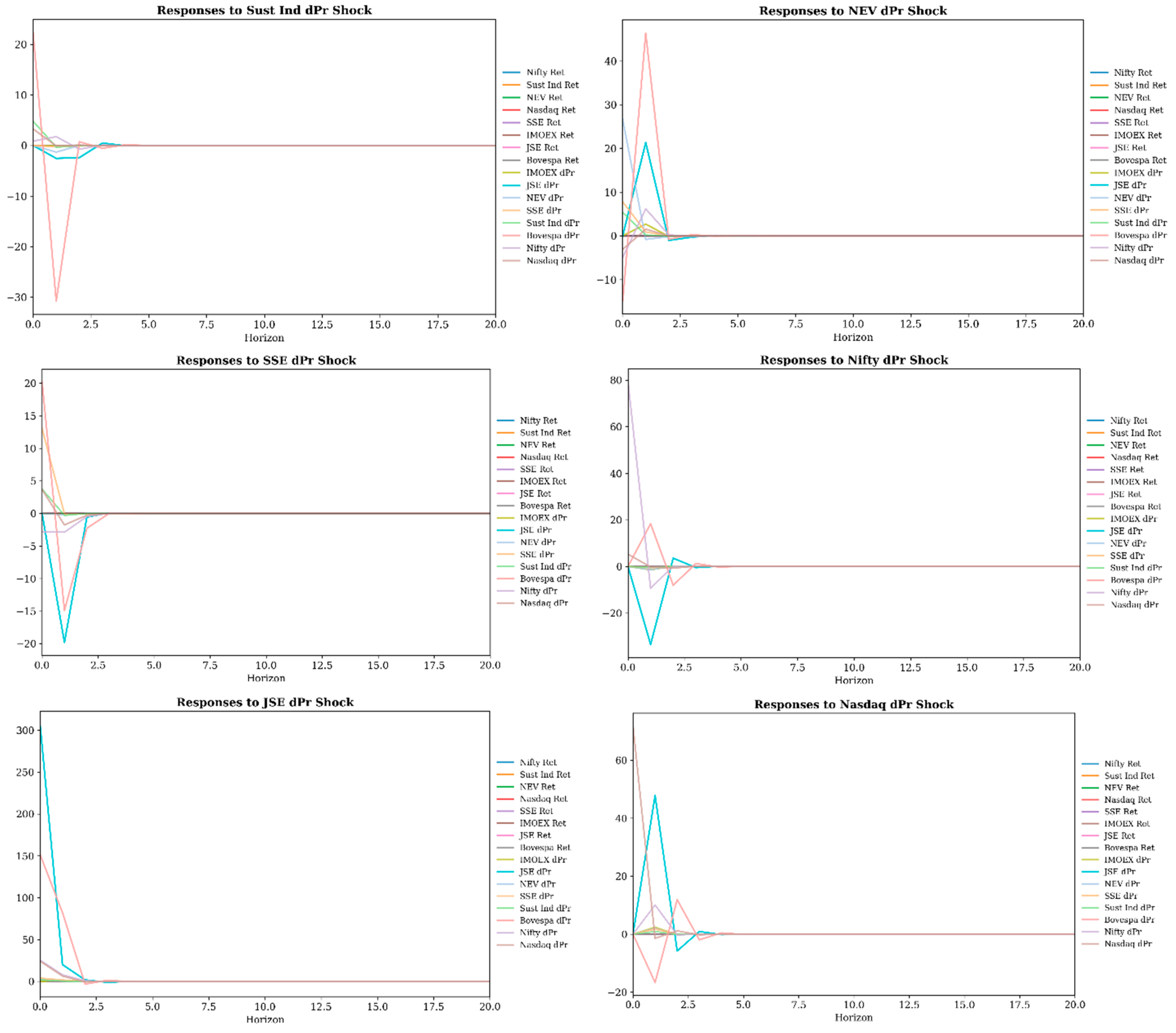
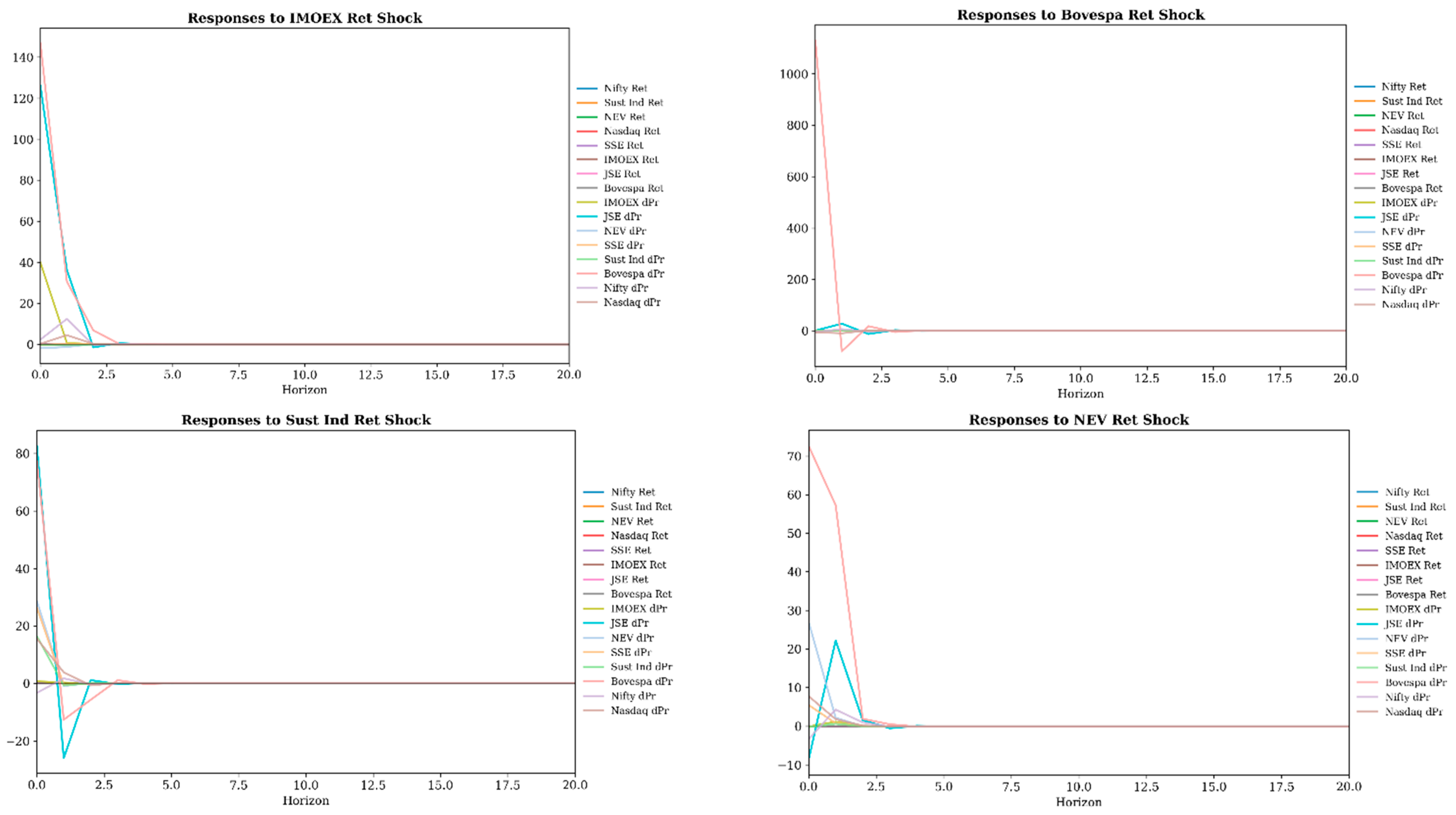
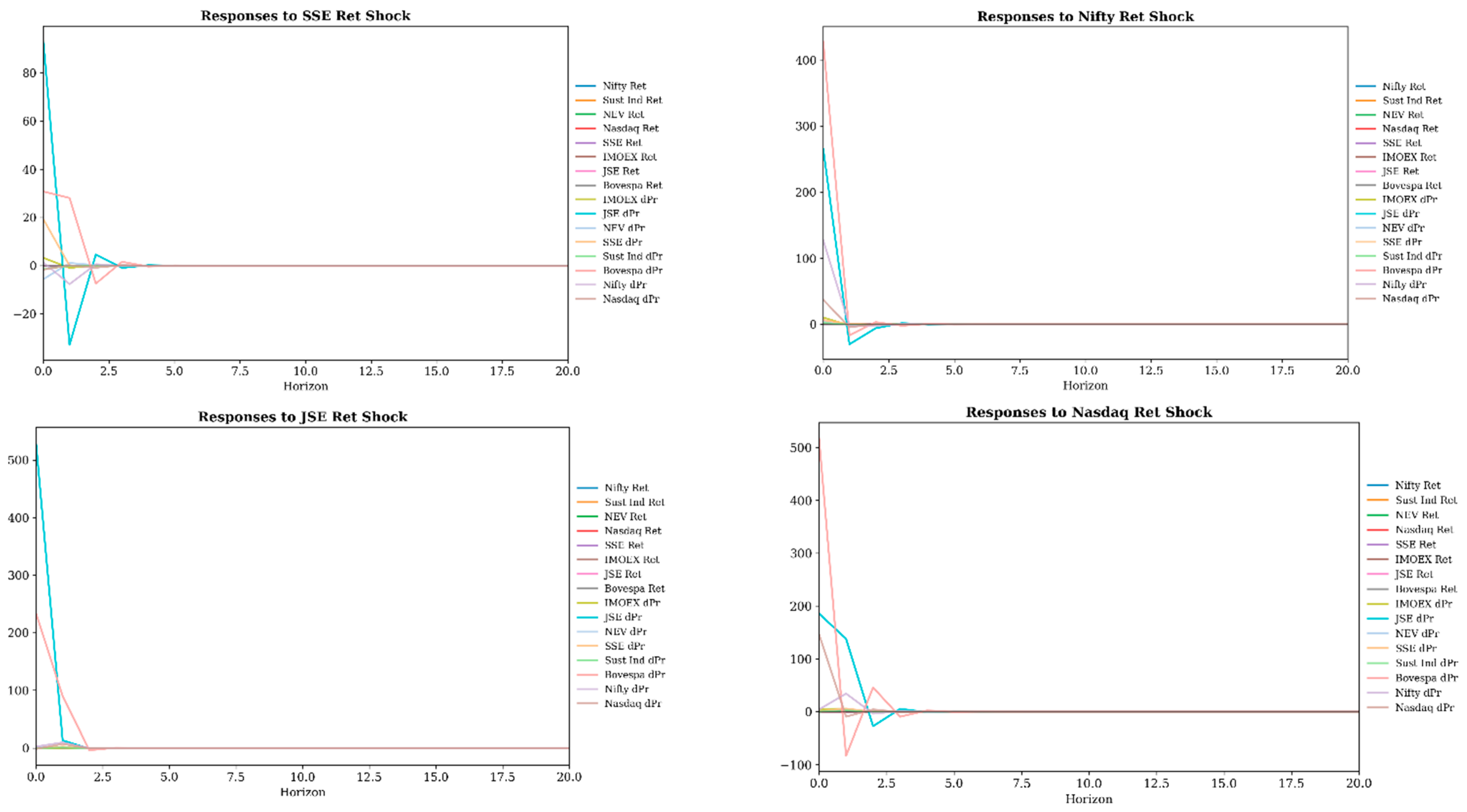
We plot impulse response functions in Figure 5 and Figure 6. The impulse responses show the following. Around 6 July 2018 (first tariff tranche), shocks from the Nasdaq and SSE to the NEV rise at impact and decay at a moderate pace, which fits trade policy transmission through technology supply chains. Around 16 March 2020 (global COVID-19 stress), shocks from the broad markets to the NEV revert faster, consistent with a temporary risk-off episode. Around 1 November 2022 (China reopening), shocks from SSE to NEV display a shorter half-life. During 2024–2025 (EV sector distress window with recalls and bankruptcy news), shocks from NEV to other markets decay slowly, which indicates persistent investor sensitivity to innovation and policy news rather than a transitory liquidity effect. Shocks from SSE ΔPrice transmit most clearly to regional partners. Nifty ΔPrice moves in close step, which signals China’s pull in Asian trade and finance. Effects on the Nasdaq appear with a delay and at smaller magnitudes. SSE return shocks rank second in size after the Nasdaq and push all return series higher, with the strongest responses in Nifty and Bovespa. SSE responses look large and persistent and decay slowly.
NEV and Sustainability index shocks travel mainly to the Nasdaq ΔPrice and returns, which points to green innovation as a leading signal for broader technology momentum. Spillovers to BRICS markets remain weak. The effects look sharp and persistent and need nearly the full horizon to revert to the mean, which fits investor focus on thematic growth. In this section, the slow decay of NEV responses signals a persistent sensitivity to innovation and policy news, whereas there were faster reversion points to short-lived liquidity or risk aversion.
JSE ΔPrice shocks act as a catalyst inside BRICS. Bovespa ΔPrice shows an immediate and strong positive response. Larger benchmarks such as Nifty and the Nasdaq respond positively but with smaller magnitudes, which places JSE in a second tier of influence within the global hierarchy. The initial impact shows a high persistence and fades gradually over a 20-period window. Other links stay small, and the impulse reverts to the mean within about 10 periods, which supports the view of JSE as a niche market, with South Africa-specific news not carrying lasting global effects. Risk tied to Russia transmits in a meaningful way to select markets, yet not across the full system.
IMOEX ΔPrice shocks hit commodity-focused markets first. The Bovespa ΔPrice jumps and JSE ΔPrice rises, while the Nasdaq ΔPrice moves only modestly. Russian news reprices Brazil and South Africa more than United States tech, so the first horizon sign agreement sits near 64 percent, consistent with partial segmentation rather than a system-wide factor. IMOEX returns confirm the near total isolation of the current regime. The impulse concentrates inside the MOEX complex, generating a large IMOEX ΔPrice response and no statistically significant effects on any other series at any horizon.
A Bovespa ΔPrice momentum shock triggers a strong sympathetic move in the JSE ΔPrice. The Nasdaq ΔPrice and Nifty ΔPrice respond with small positive shifts, and domestic returns rise. The pattern emerges quickly and then decays within five to seven periods, which suggests that markets trade Bovespa news aggressively and treat it as transient rather than as a signal of broader fundamentals.
The Indian momentum shock shows a dual profile: strong regional transmission with little global reach. JSE ΔPrice and Bovespa ΔPrice register immediate positive responses, and Nifty returns display the same behavior. Nifty returns also lift SSE returns in a modest yet clear way, which points to a competitive but linked relationship between the two large Asian markets.

4.3. Dynamic Connectedness with TVP-VAR Model

The TVP VAR and LASSO results corroborate the BVAR evidence on links between China’s green sector and BRICS markets. The Total Connectedness Index in Figure 7 stays high, yet the trend moves lower over time. In 2020, the first large shock was linked to the pandemic lift’s connectedness, from 76 percent in February to 83 percent in April. The series then resumes a downward path. Later global events leave a smaller mark, with one clear exception in April 2025: connectedness jumps by about 7 percent, likely tied to new United States tariffs and reports of overheating and bankruptcies in parts of China’s green technology sector.
The declining path points to weaker links among BRICS financial markets despite ambitions for closer political and economic coordination. Figure 8 charts the NET dynamic connectedness and clarifies who sends volatility and who absorbs it. The Nasdaq ranks as the largest transmitter, followed by Bovespa, JSE ΔPrice, Sustainable Industry, and SSE. Nifty returns and IMOEX returns stand out as the main recipients.
Sustainable Industry mostly transmits risk, though its role flips during the pandemic. NEV ΔPrice shifts into a transmitter role near the end of 2024, in step with the rising trade war risk in 2025, whereas NEV returns alternate between sending and receiving across the sample. Nifty consistently absorbs shocks across the horizon. The Nasdaq moves from a transmitter to a recipient in the later years for both ΔPrice and returns. JSE, especially ΔPrice, transmits sizable shares of volatility throughout. Bovespa prices and returns behave as transmitters for most of the sample, with returns switching to a recipient role in 2025. IMOEX prices and returns show brief transmission spells after 2022, yet for much of the period they absorb shocks. The SSE Composite shows a similar split: ΔPrice turns into a transmitter after 2020 and returns adopt that role in 2024.
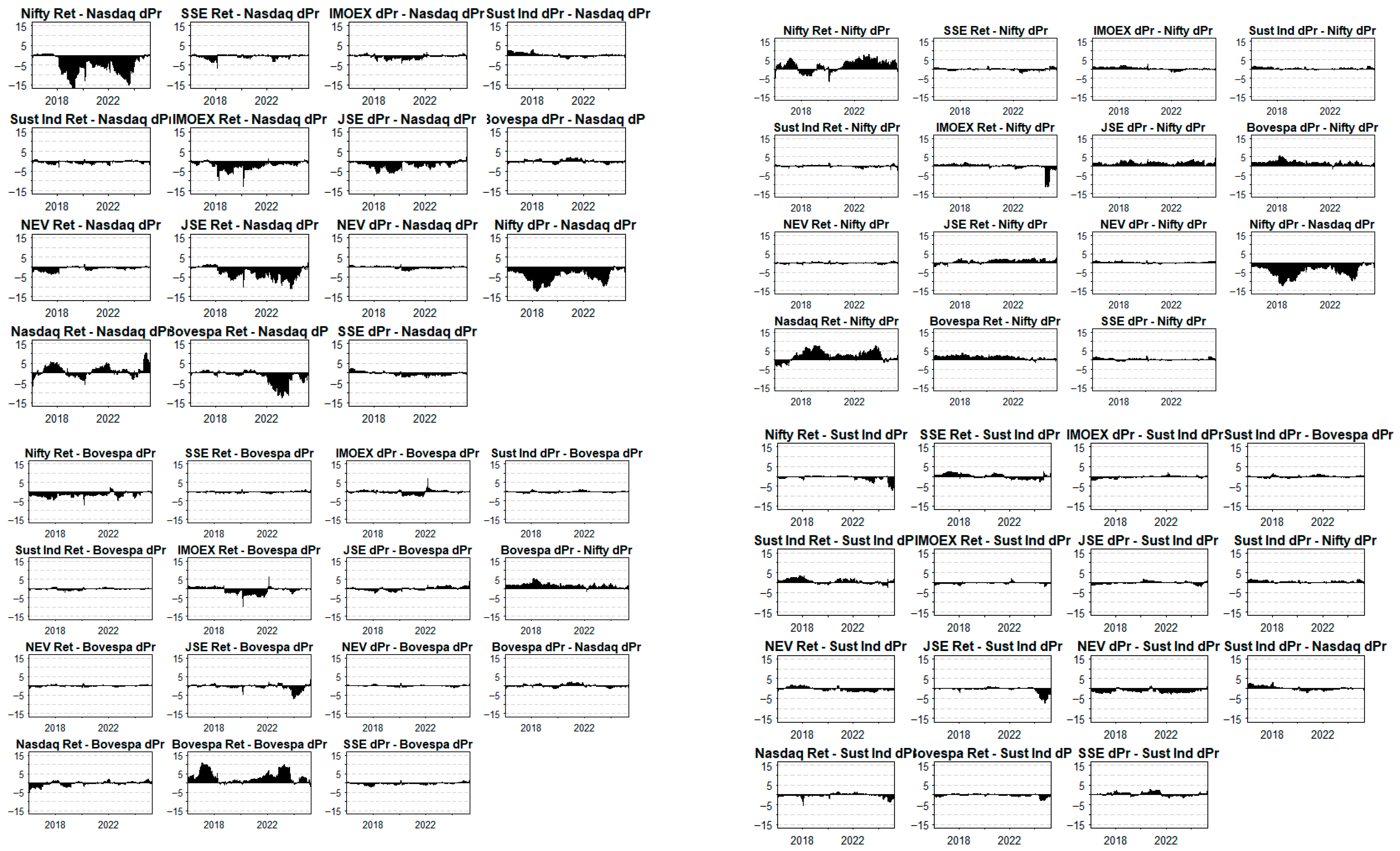
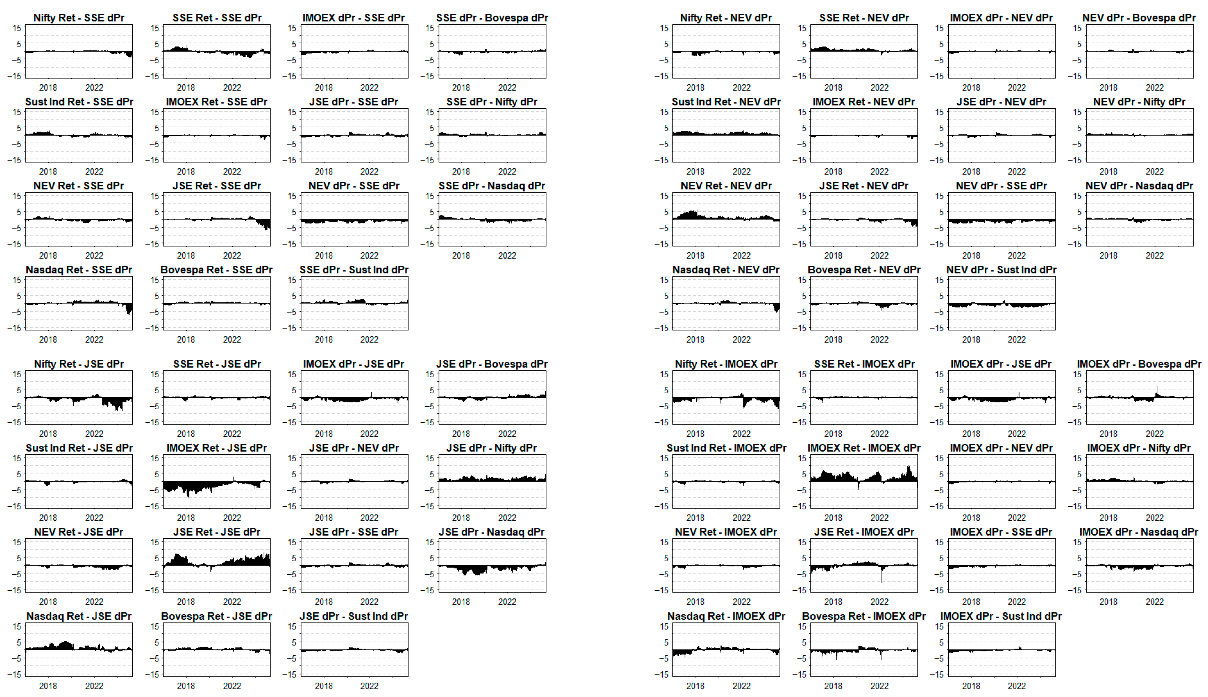
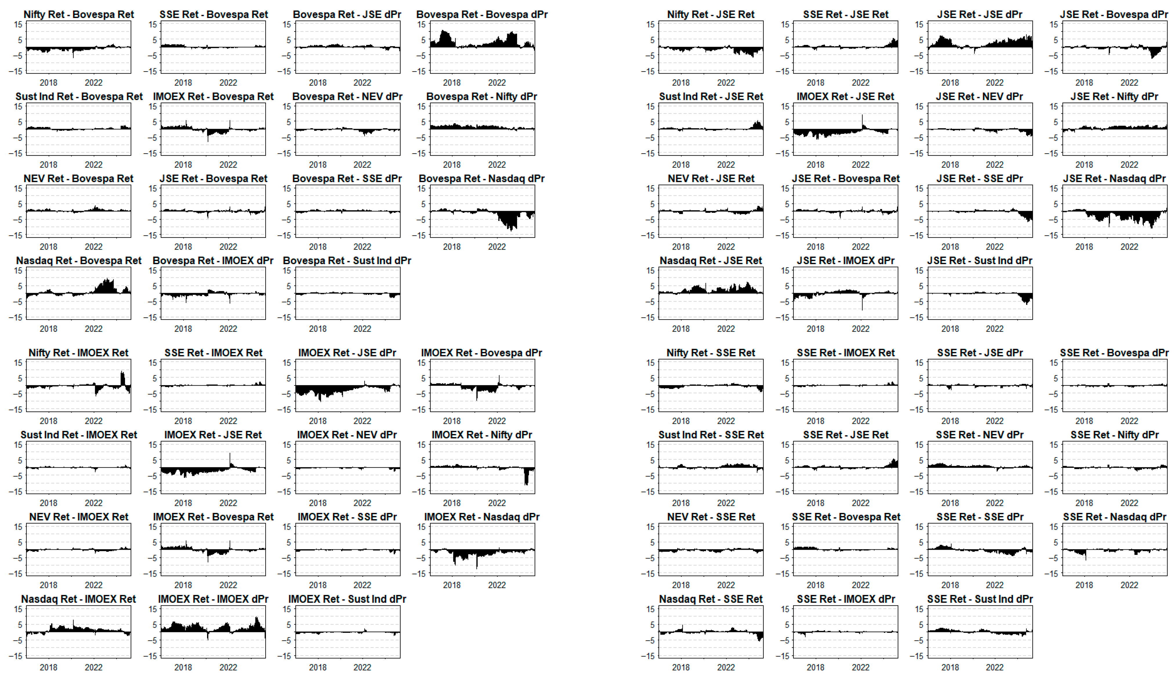
Figure A5, Figure A6, Figure A7 and Figure A8 in Appendix A plot pairwise dynamic interconnectedness across all variables. Nifty prices and returns appear among the most affected series, with the Nasdaq, Bovespa, JSE, and later IMOEX providing the largest inputs. SSE prices and returns contribute little to spillovers, and the green indices contribute the least within this set. IMOEX mostly receives shocks from Bovespa, JSE, Nasdaq prices, and China’s green sector, then passes part of that risk to Nifty, Nasdaq, and SSE. The green complex cycles through regimes with limited influence at first. NEV and Sustainable Industry, for both ΔPrice and returns, start to transmit risk from 2024 onward, which aligns with trade and election headlines in the run up to 2025 and shows most clearly in links with JSE, IMOEX, Bovespa, and Nifty. NEV’s later move into transmission likely stems from its narrower industry base compared with Sustainable Industry, which spans renewables, waste, utilities, and related activities. Spillover patterns in the green set after 2022 mirror the shocks that SSE sends or receives vis-a-vis other BRICS indices, and on a pairwise scale the green indices tend to receive shocks from SSE.
To reconcile the historical pattern with the late-sample shift, we define ‘niche’ as a lower time-average connectedness centrality, negative mean NET over 2016–2024, and narrow counterparties. In early–mid 2025, NEV registers brief net-transmitter spells coinciding with tariff and bankruptcy news. A change-in-mean test on NET(NEV) confirms that 2025 values differ from the 2016–2024 distribution, yet the spells cover a small share of total observations, so they indicate episodic integration rather than a full regime replacement.
To test for redundancy and sharpen inference, the study adds LASSO variable selection (Table 4) (Fefelov et al. 2025). LASSO applies an L1 penalty that shrinks weak coefficients toward zero, which improves prediction and clarifies the set of informative predictors (Tateishi et al. 2010).
The NET and NPT coefficients of the LASSO model are either positive or negative, significantly different from zero, which allows us to include all the variables into the model. The NET value represents the strength and direction of the relationship between each predictor variable. NPT (order of model entry) indicates the order in which the variable entered the model as the regularization penalty was relieved. A lower number means that it was considered important very early, while the value of zero means the lack of informativeness of the variable. The LASSO results confirm NEV and Sustainable Industry as late-entry volatility transmitters (NPT ranging from 10 to 13), underscoring the increasing systemic relevance of the green sector post-2024.

5. Discussion

The analysis yields multifaceted evidence on volatility spillovers in the BRICS–China green–Nasdaq system using ΔPrice and returns. Both models report an initially high level of connectedness that then declines through 2016–2025, interrupted by one large shock during COVID-19 and several smaller shocks across the sample (Table 5).
After the pandemic, the declining trend resumes, which points to a decoupling phase as economies prioritize domestic resilience, similar to the post-2013 period when emerging markets reduced their exposure to external shocks (Lòpez-Villavicencio and Pourroy 2022). BRICS members pursue foreign reserve accumulation and settle a larger share of payments in local currencies to reduce their dependence on Western markets. Evidence also shows a decoupling inside BRICS. As a group, BRICS has not achieved deep financial or policy integration. Local currency trade remains small, and the National Development Bank faces internal constraints tied to sanctions, limited capital, and China’s dominant position (Duggan et al. 2022). Risk management therefore is manifested in insulation not only from Western markets but also from partners in emerging markets.
Market roles separate clearly. JSE, Bovespa, and post-2022 Russia emerge as net transmitters of volatility, in line with variance breakpoints, although TVP VAR results show that IMOEX shocks eventually fade. Nifty acts as the main recipient, which signals a high sensitivity to external news. China’s green stocks display distinct high-volatility regimes steered by policy themes and climate sentiment, as during the pandemic period (Ye et al. 2025). The GFEVD matrix shows that these indices, ΔPrice and returns, sit among the most isolated in the sample, with links concentrated on the Nasdaq and SSE. Green assets therefore still trade as a financial niche despite their growth in scale and relevance, and China’s green stocks remain driven by domestic factors and national policy (Yiming et al. 2024). The SSE Composite also appears isolated from other BRICS markets, which fits the segmented market dynamics in China (Sher et al. 2024).
We also record a wave of moderate shocks and a jump in the BVAR-based TCI to 66.13 percent in April 2025. In principle, a rise of this sort might hint at a broadening role for green assets, yet prior evidence shows that disruptive news can lift connectedness temporarily and then retreat to prior, even more segmented states (Wang et al. 2024). The pattern calls for longer samples to confirm persistence.
Impulse responses add regional detail. SSE spillovers hit India the hardest, and the green sector channels influence almost exclusively to the Nasdaq, which supports a thematic rather than a global or geopolitical footprint. A regional core inside BRICS links JSE, Bovespa, and Nifty through strong two-way spillovers that align with shared commodity and macro risk factors (Bhuyan et al. 2016).
The declining TCI points to a weaker financial integration, which fits the divergent monetary policies, geopolitical frictions, and domestic reforms. Investor behavior does not mirror political narratives about a unified BRICS front. The setting echoes the 2012 solar industry crash, when an excess capacity and trade barriers disrupted renewable supply chains (Green and Newman 2017). Commodity-driven markets act as primary shock sources in our sample (Mensi et al. 2023; Fefelov et al. 2025). Alternative energy stocks mostly receive volatility rather than transmit it across the period studied.
Sustainable Industry shows a higher volatility and connectedness than NEV because the two indices differ in scope and exposure. Both indices are thematic, yet Sustainable Industry spans energy efficiency, sustainable materials, waste management, and green technology. This breadth expands exposure to policy shocks and shifts in sustainability sentiment across multiple channels. NEV concentrates on electric vehicles, batteries, and related supply chains. The segment faces intense competition, rapid technological turnover, and a heightened sensitivity to targeted geopolitical risks, including US–China trade measures on electric vehicles and critical minerals. NEV therefore acts as a net receiver of shocks through most samples. In late 2024, it turns into a net transmitter in both the TVP VAR and LASSO results, consistent with market pricing expected for trade conflicts and sector-wide repricing that sends volatility to adjacent assets.

6. Theoretical Contribution

Our study advances evidence on volatility spillovers in green and emerging markets. Crises often lift volatility across markets at the same time (Diebold and Yilmaz 2012), yet in this sample only the COVID-19 pandemic fits that pattern. Later shocks tied to geopolitics and trade stay more localized, which points to regionalization and segmentation consistent with asymmetric spillover evidence (Baruník et al. 2016). These results challenge strong form efficiency and support segmented market views and home bias among BRICS investors (Coudert et al. 2015). China’s green stocks shape domestic pricing more than BRICS linkages. Events that strike green policy or production (pandemics or targeted tariffs) carry farther and trigger sector-wide repricing, which raises the chance that the green complex becomes a source of volatility as global reliance on Chinese green technology grows. Green assets still hedge energy risk better than commodities such as gold, with a weaker correlation to oil in high-climate-risk states (Yuan et al. 2023).

7. Practical Contributions

Our study is useful for investors, financial analytics, and economists. Economic uncertainty, combined with crises and tensions, results in the decoupling of international financial markets from each other. Green assets, despite the increasing targeting by tariffs, remain an effective hedge strategy and can be used to form a risk-resilient portfolio. Investors from developed economies should monitor policies and event-specific news which can cause and propagate shocks. Given the event-sensitive transmitter spells in 2025, policy communication and tariff timing can amplify or dampen the sector’s system impact. Sustained transmitter status should be reassessed as new data accrues.

8. Conclusions

Evidence points to a historically peripheral role of green indices between 2016 and 2024. Since mid-2025, event-linked transmitter episodes appear (mostly for NEV) and suggest early integration rather than a settled reclassification of the sector’s network role. The results show a secular decline in the Total Connectedness Index, a pattern consistent with market segmentation and a weaker cross-market transmission. China’s green indices retain a niche profile in global finance, yet episodes tied to policy and trade shift their footprint and lift their influence on technology benchmarks. Evidence on asymmetric responses and short-lived spikes around major shocks points to a transmission that depends on policy cycles, trade measures, and climate related news. Future work can extend this framework with finer sector splits, firm level disclosures, and a higher-frequency identification of structural breaks to test whether green assets continue to gain systemic relevance as trade frictions and green technology exports expand.

9. Limitations

China’s green sector ranks among the most developed, and the BRICS markets in this study include some of the largest economies, yet evidence from other settings remains necessary. The EU’s green sector may transmit more volatility given the recent energy crisis. Several results on the role of green assets need follow-up as trade conflicts evolve. The design relies on VAR models, which may understate volatility dynamics. Future work can apply multivariate GARCH families and wavelet methods to test robustness and to separate spillovers by horizon.

Author Contributions

Conceptualization, D.B.V. and D.L.F.; methodology, D.B.V. and D.L.F.; software, D.L.F.; validation, E.M.R. and D.B.V.; formal analysis, D.L.F. and D.B.V.; investigation, D.B.V., D.L.F. and M.F.; resources, E.M.R.; data curation, D.L.F.; writing—original draft preparation, D.B.V. and D.L.F.; writing—review and editing, M.F., E.M.R. and D.B.V.; visualization, D.L.F.; supervision, D.B.V.; project administration, E.M.R.; funding acquisition, D.B.V., D.L.F. and E.M.R. All authors have read and agreed to the published version of the manuscript.

Funding

The work of authors has been supported by the Russian Science Foundation grant for the project “Market efficiency in turmoil: an arbitrage opportunity and a relative optimization in the long run”, project No. 24-28-00521.

Institutional Review Board Statement

This article does not contain any studies with human participants performed by any of the authors.

Data Availability Statement

To support transparency and replication, we share full lists of tickers, exact sampling windows, and the transformation scripts used to construct the analysis dataset, and we post all derived outputs. The underlying market series are sourced from licensed vendors (Wind Terminal and Investing.com). Our institutional agreements restrict redistribution of downloaded histories, even when prices are publicly observable on exchanges, so we cannot post the raw files. Qualified readers who have legitimate access to these sources can recreate the dataset using our materials.

Conflicts of Interest

The authors declare no conflicts of interest.

Appendix A

Formula (A1). VAR(1) baseline (stationary)
y t = c + A 1 y t 1 + ε t , ε t ~ ( 0 , Σ ε )
where y t is a (16 × 1) vector of endogenous variables (eight markets × {ΔPrice, Returns}) in the full sample window; c is a (16 × 1) intercept; A1 is a (16 × 16) lag-one coefficient matrix (p = 1); ε t is a (16 × 1) vector of innovations; and Σ ε is a (16 × 16) positive-definite innovation covariance matrix.
Formula (A2). Moving-average (∞) representation and Ψ recursion
y t = μ + h = 0 Ψ h   ε t h
Ψ 0 = I ,   Ψ h = A 1   Ψ h 1   ( h 1 )
where μ is the (n × 1) unconditional mean; Ψ0 = In and Ψ h (n × n) are the impulse-response matrices at horizon h; and the recursion with A1 links the innovations to future outcomes.
Formula (A3). Generalized impulse responses (GIRFs)
G I R F i j ( h ) = σ j j 1 / 2   ( e i   Ψ h   Σ ε   e j )
where G I R F i j ( h ) is the response of variable i at horizon h to a generalized unit shock in variable j; e i and e j are canonical selection vectors; Ψ h is the (n × n) impulse-response matrix; and Σ ε is the innovation covariance, with σ j j 1 / 2 on its diagonal.
Formula (A4). Generalized FEVD (H = 10) and row-normalization
θ i j ( 10 ) = σ j j 1   h = 0 9 ( e i   Ψ h   Σ ε   e j ) 2 h = 0 9 ( e i   Ψ h   Σ ε   Ψ h   e i )
~ θ i j ( 10 ) = θ i j ( 10 ) j = 1 N θ i j ( 10 ) ,   j = 1 N ~ θ i j ( 10 ) = 1
where θ i j ( 10 ) is the H = 10 generalized FEVD share from shocks in j to the forecast error variance of i; and ~ θ i j ( 10 ) row-normalizes these contributions so that they sum to one across j for each i.
Formula (A5). System-wide and directional connectedness (N = 16, H = 10)
T C I ( 10 ) = 100 · 1 16 · i = 1 16 j i ~ θ i j ( 10 )
C i · ( 10 ) = 100 · ~ θ i j ( 10 ) ,   j i
C i · ( 10 ) = 100 · ~ θ j i ( 10 ) ,   j i
C i n e t ( 10 ) = C i · ( 10 ) C i · ( 10 )
where TCI(10) is the average off-diagonal share (in %) across the 16-variable system; C i · ( 10 ) (from) aggregates contributions received by i; C i · ( 10 ) (to) aggregates contributions transmitted by i; and C i n e t ( 10 ) = to − from identifies net transmitters and recipients. Empirically, the ΔPrice+Returns specification yields economically large TCI values, with distinct regime variation and stable NET rankings across windows.
Formula (A6). Bootstrap confidence intervals for IRFs (H = 20)
C I i j ( 20 ) = [ G I R F i j ( 20 ) ( q α / 2 ) , G I R F i j ( 20 ) ( q 1 α / 2 ) ]
where C I i j ( 20 ) is the equal-tailed percentile interval for GIRFs at horizon 0–20 based on bootstrap quantiles q k . Such an approach accommodates non-Gaussian residual features typical of daily data and anchors uncertainty around the generalized responses.
Formula (A7). Structural-break dating and uncertainty
C I τ   b = [ q α / 2 ( τ b * ) , q 1 α / 2 ( τ b * ) ]
where τ b denotes a break date identified by binary segmentation under a BIC criterion and τ b * are bootstrap estimates from moving-block resamples; and C I τ   b is the equal-tailed interval based on the empirical distribution of τ b * . Our procedure is applied to the TCI mean and series-level variances, linking regime changes to volatility spikes observed in rolling connectedness.
Formula (A8). Bayesian Ridge/Minnesota prior
E [ a i i , 1 ] = 1 ,   E [ a i j , l ] = 0   ( i j   \   o r   \   l 2 ) V a r ( a i j , l ) = γ 2 · σ i 2 σ j 2 · 1 l 2
where a i i , 1 is the coefficient of variable j at lag l in equation i; E [ a i i , 1 ] = 1 and other coefficients have zero mean; and V a r ( a i j , l ) scales with γ2 (overall tightness), the variance ratio σ i 2 σ j 2 , and 1 l 2 lag decay. We tune γ ∈ {0.05, 0.10, 0.20, 0.50, 1.00, 2.00, 5.00} via out-of-sample log scores; γ = 5.00 is optimal in both windows, stabilizing estimates while preserving spillover rankings relative to the unrestricted VAR. Additionally, we conducted diagnostic checks to confirm VAR stability and standard daily data features (Table 3).
The evolving dynamic connectedness between variables m and n at any given time t within the TVP-VAR model can be mathematically expressed as follows:
Formula (A9). TVP-VAR-based Dynamic Connectedness Approach
D m n , t = 1 1 + l = 1 q B m n , l ( t )
where D m n , t signifies the dynamic connectedness between variables m and n at time t, the summation over l captures the cumulative influence of the time-varying coefficients on the connectedness measure, and the absolute values of the coefficients, denoted by B m n , l ( t ) , represent the strength of the influence between variables at lag order l.
Formula (A10). TVP-VAR model
Z t = m = 1 q B m t Z t m + v t ,  
B m t = B m t 1 + θ m t ,
where the vector of variables at time t is denoted by Z t , time-varying coefficient matrices are represented by B m t , the error term at time t is denoted by v t , and the parameters are updated based on stochastic shocks, represented by noise terms θ m t .
Formula (A11). LASSO model
ζ t = α + m = 1 q B m Z t m + Λ m = 1 q β m ,  
where ζ t denotes the predicted value of the vector of variables at time t, α is the intercept term, β m represents the coefficients for the lagged values of the variables, Z t m denotes the vector of variables at lag m, λ is the regularization parameter that controls the degree of shrinkage applied to the coefficients β m , and the term m = 1 q β m is the L1 norm, which imposes a penalty proportional to the absolute values of the coefficients, encouraging sparsity. According to the last, the LASSO model aims to minimize the residual sum of squares subject to the L1 norm penalty, formulated as follows:
m i n α , β t 1 T Z t α m = 1 q B m Z t m 2 + Λ m = 1 q β m ,
where T is the total number of time periods in the dataset.
Table A1. Stationarity checks (KPSS).
SeriesPricep-Value (Price)KPSS (Returns)p-Value (Returns)KPSS Stat (ΔPrice)p-Value (ΔPrice)
Nifty19.2120.010.0591640.10.105530.1
Sust Ind8.17150.010.219240.10.184320.1
NEV3.8790.010.247130.10.186010.1
Nasdaq18.3560.010.0347780.10.0503480.1
SSE2.26270.010.0485190.10.0346460.1
IMOEX8.52170.010.104450.10.0728010.1
JSE17.540.010.0524210.10.0679090.1
Bovespa17.4750.010.293880.10.0490650.1
Table A2. TO, FROM, and NET connectedness coefficients.
SeriesFROMTONET
Nasdaq Ret62.984268.70365.7195
Sust Ind Ret75.263480.7575.4936
JSE Ret68.531673.30464.773
JSE ΔPr68.484672.9424.4574
Nasdaq ΔPr61.34265.49184.1498
Bovespa ΔPr64.798468.88954.0912
SSE Ret75.113579.15734.0439
SSE ΔPr74.897278.4283.5308
Bovespa Ret64.147965.87451.7266
Sust Ind ΔPr73.981875.06041.0786
NEV Ret72.953772.3506−0.6031
IMOEX ΔPr57.777953.1984−4.5796
IMOEX Ret57.662752.7991−4.8636
Nifty Ret63.184655.6447−7.5399
Nifty ΔPr62.217651.8665−10.3511
NEV ΔPr68.980957.8538−11.1271
Table A3. Bayesian VAR prior tightness (γ) grid and predictive performance.
GammaAverage Log ScoreEvaluations
5−23.4133940
2−23.4128940
1−23.4126940
0.5−23.4132940
0.2−23.4196940
0.1−23.4338940
Figure A1. Variance breakpoints and segmentations (ΔPrices).
Risks 13 00222 g0a1aRisks 13 00222 g0a1b
Figure A2. Variance breakpoints and segmentations (returns).
Risks 13 00222 g0a2
Figure A3. Impulse response plots (ΔPrices).
Risks 13 00222 g0a3aRisks 13 00222 g0a3b
Figure A4. Impulse response plots (returns).
Risks 13 00222 g0a4aRisks 13 00222 g0a4b
Figure A5. Net pairwise dynamic connectedness plot (1).
Risks 13 00222 g0a5
Figure A6. Net pairwise dynamic connectedness plot (2).
Risks 13 00222 g0a6
Figure A7. Net pairwise dynamic connectedness plot (3).
Risks 13 00222 g0a7
Figure A8. Net pairwise dynamic connectedness plot (4).
Risks 13 00222 g0a8

References

  1. Alsahlawi, Abdulaziz Mohammed, Kaouther Chebbi, and Mohammed Abdullah Ammer. 2021. The impact of environmental sustainability disclosure on stock return of Saudi listed firms: The moderating role of financial constraints. International Journal of Financial Studies 9: 4. [Google Scholar] [CrossRef]
  2. Antonakakis, Nikolaos, David Gabauer, and Rangan Gupta. 2019. International monetary policy spillovers: Evidence from a time-varying parameter vector autoregression. International Review of Financial Analysis 65: 101382. [Google Scholar] [CrossRef]
  3. Araújo, Deborah. 2025. Brazil and China Sign Billion-Dollar Deals to Explore Lithium and Rare Earths in South America, Challenging U.S. Dominance in the Energy Transition. CPG. Available online: https://en.clickpetroleoegas.com.br/Brazil-and-China-sign-billion-dollar-agreements-to-explore-lithium-and-rare-earths-in-South-America-and-challenge-US-dominance-in-the-energy-transition-dsca00/ (accessed on 19 October 2025).
  4. Baruník, Jozef, Evžen Kočenda, and Lukáš Vácha. 2016. Volatility spillovers across petroleum markets. The Energy Journal 37: 136–58. [Google Scholar] [CrossRef]
  5. Bhuyan, Rafiqul, Mohammad G. Robbani, Bakhtear Talukdar, and Ajeet Jain. 2016. Information transmission and dynamics of stock price movements: An empirical analysis of BRICS and US stock markets. International Review of Economics & Finance 46: 180–95. [Google Scholar] [CrossRef]
  6. Busse, Jeffrey A., and T. Clifton Green. 2002. Market efficiency in real time. Journal of Financial Economics 65: 415–37. [Google Scholar] [CrossRef]
  7. Chan, Bonnie Y. 2025. How China is Helping Power the World’s Green Transition. World Economic Forum. Available online: https://www.weforum.org/stories/2025/01/why-china-matters-to-the-worlds-green-transition/ (accessed on 9 June 2025).
  8. Chițimiea, Andreea, Mihaela Minciu, Andreea-Mariana Manta, Carmen Nadia Ciocoiu, and Cristina Veith. 2021. The drivers of green investment: A bibliometric and systematic review. Sustainability 13: 3507. [Google Scholar] [CrossRef]
  9. Coudert, Virginie, Karine Hervé, and Pierre Mabille. 2015. Internationalization versus regionalization in the emerging stock markets. International Journal of Finance & Economics 20: 16–27. [Google Scholar]
  10. Dev, Rhea. 2025. Trump’s Paris agreement withdrawal risks global crisis. Green Left 1423: 12. [Google Scholar]
  11. Diebold, Francis X., and Kamil Yilmaz. 2012. Better to give than to receive: Predictive directional measurement of volatility spillovers. International Journal of Forecasting 28: 57–66. [Google Scholar] [CrossRef]
  12. Ding, Xiaowei, Darko B. Vuković, Boris I. Sokolov, Natalia Vukovic, and Yali Liu. 2024. Enhancing ESG performance through digital transformation: Insights from China’s manufacturing sector. Technology in Society 79: 102753. [Google Scholar] [CrossRef]
  13. Ding, Xiuying, and Xuemei Liu. 2023. Renewable energy development and transportation infrastructure matters for green economic growth? Empirical evidence from China. Economic Analysis and Policy 79: 634–46. [Google Scholar] [CrossRef]
  14. Duggan, Niall, Juan Carlos Ladines Azalia, and Marek Rewizorski. 2022. The structural power of the BRICS (Brazil, Russia, India, China and South Africa) in multilateral development finance: A case study of the New Development Bank. International Political Science Review 43: 495–511. [Google Scholar] [CrossRef]
  15. Fama, Eugene F. 1970. Efficient capital markets: A review of theory and empirical work. The Journal of Finance 25: 383–417. [Google Scholar] [CrossRef]
  16. Fefelov, Dmitrii, Elena Rogova, and Darko Vukovic. 2025. Assessing the financial interconnectedness between China and Russia: A dynamic approach. Journal of the New Economic Association 67: 110–37. [Google Scholar] [CrossRef]
  17. Galbraith, John W., and Serguei Zernov. 2009. Extreme dependence in the NASDAQ and S&P 500 composite indexes. Applied Financial Economics 19: 1019–28. [Google Scholar]
  18. Gao, Yang, Chengjie Zhao, Bianxia Sun, and Wandi Zhao. 2022. Effects of investor sentiment on stock volatility: New evidences from multi-source data in China’s green stock markets. Financial Innovation 8: 77. [Google Scholar] [CrossRef] [PubMed]
  19. Global Times. 2024. GT Voice: BRICS’ Green Devt Offers New Path for Global Energy Transition. Global Times. Available online: https://www.globaltimes.cn/page/202410/1321691.shtml (accessed on 5 June 2025).
  20. Green, Jemma, and Peter Newman. 2017. Disruptive innovation, stranded assets and forecasting: The rise and rise of renewable energy. Journal of Sustainable Finance & Investment 7: 169–87. [Google Scholar]
  21. Ha, Le Thanh. 2024. A wavelet analysis of dynamic connectedness between geopolitical risk and renewable energy volatility during the COVID-19 pandemic and Ukraine-Russia conflicts. Environmental Science and Pollution Research 31: 17994–8009. [Google Scholar] [CrossRef]
  22. Handley, Kyle, Fariha Kamal, and Ryan Monarch. 2025. Rising import tariffs, falling exports: When modern supply chains meet old-style protectionism. American Economic Journal: Applied Economics 17: 208–38. [Google Scholar] [CrossRef]
  23. He, Zheng, Zhengkai Liu, Congzhi Zhang, and Yuanjun Zhao. 2025. How do carbon pricing spillover effects impact green asset price volatility? An empirical study based on the TVP-VAR-DY model. Economic Analysis and Policy 85: 2162–79. [Google Scholar] [CrossRef]
  24. Investing.com. 2025. Investing.com. Available online: https://www.investing.com/ (accessed on 5 June 2025).
  25. Jiang, George J., Eirini Konstantinidi, and George Skiadopoulos. 2012. Volatility spillovers and the effect of news announcements. Journal of Banking & Finance 36: 2260–73. [Google Scholar] [CrossRef]
  26. Khalfaoui, Rabeh, Mohamed Boutahar, and Heni Boubaker. 2015. Analyzing volatility spillovers and hedging between oil and stock markets: Evidence from wavelet analysis. Energy Economics 49: 540–49. [Google Scholar] [CrossRef]
  27. Lin, Boqiang, and Zhizhou Tan. 2023. Exploring arbitrage opportunities between China’s carbon markets based on statistical arbitrage pairs trading strategy. Environmental Impact Assessment Review 99: 107041. [Google Scholar] [CrossRef]
  28. Lin, Jiun-Da. 2023. Explaining the quality of green bonds in China. Journal of Cleaner Production 406: 136893. [Google Scholar] [CrossRef]
  29. Liu, Min, Tongji Guo, Weiying Ping, and Liangqing Luo. 2023. Sustainability and stability: Will ESG investment reduce the return and volatility spillover effects across the Chinese financial market? Energy Economics 121: 106674. [Google Scholar] [CrossRef]
  30. Lòpez-Villavicencio, Antonia, and Marc Pourroy. 2022. Fed’s policy changes and inflation in emerging markets: Lessons from the taper tantrum. Journal of Money, Credit and Banking 54: 1099–121. [Google Scholar] [CrossRef]
  31. Lundgren, Amanda Ivarsson, Adriana Milicevic, Gazi Salah Uddin, and Sang Hoon Kang. 2018. Connectedness network and dependence structure mechanism in green investments. Energy Economics 72: 145–53. [Google Scholar] [CrossRef]
  32. McMillan, David G., and Alan EH Speight. 2010. Return and volatility spillovers in three euro exchange rates. Journal of Economics and Business 62: 79–93. [Google Scholar] [CrossRef]
  33. Mensi, Walid, Muhammad Shafiullah, Xuan Vinh Vo, and Sang Hoon Kang. 2021. Volatility spillovers between strategic commodity futures and stock markets and portfolio implications: Evidence from developed and emerging economies. Resources Policy 71: 102002. [Google Scholar] [CrossRef]
  34. Mensi, Walid, Xuan Vinh Vo, Hee-Un Ko, and Sang Hoon Kang. 2023. Frequency spillovers between green bonds, global factors and stock market before and during COVID-19 crisis. Economic Analysis and Policy 77: 558–80. [Google Scholar] [CrossRef] [PubMed]
  35. Myllyvirta, Lauri, Qi Qin, and Chengcheng Qiu. 2025. Analysis: Clean Energy Contributed a Record 10% of China’s GΔPRGΔPR in 2024. Centre of Research on Energy and Clean Air. Available online: https://energyandcleanair.org/analysis-clean-energy-contributed-a-record-10-of-chinas-gdp-in-2024/ (accessed on 19 October 2025).
  36. OECD. 2024. Climate Adaptation Investment Framework. Green Finance and Investment. Paris: OECD Publishing. [Google Scholar] [CrossRef]
  37. Papathanasiou, Spyros, and Drosos Koutsokostas. 2024. A trade-off between sustainability ratings and volatility in portfolio hedging strategies. International Journal of Banking, Accounting and Finance 14: 370–406. [Google Scholar] [CrossRef]
  38. Reuters. 2025. Chinese EV Maker Hozon Enters Bankruptcy Proceedings, State Media Reports. Reuters. Available online: https://www.reuters.com/legal/litigation/chinese-ev-maker-hozon-enters-bankruptcy-proceedings-state-media-reports-2025-06-20/ (accessed on 19 October 2025).
  39. Shen, Chen, Shenglan Li, Xiaopeng Wang, and Zhongju Liao. 2020. The effect of environmental policy tools on regional green innovation: Evidence from China. Journal of Cleaner Production 254: 120122. [Google Scholar] [CrossRef]
  40. Sher, Azmat, An Haizhong, Muhammad Kaleem Khan, and Judit Sági. 2024. Chinese stock market integration with developed world: A portfolio diversification analysis. Heliyon 10: e29413. [Google Scholar] [CrossRef]
  41. Siddique, Md Abubakar, Haitham Nobanee, Md Bokhtiar Hasan, Gazi Salah Uddin, and Md Nahiduzzaman. 2024. Is investing in green assets costlier? Green vs. non-green financial assets. International Review of Economics & Finance 92: 1460–81. [Google Scholar] [CrossRef]
  42. Tateishi, Shohei, Hidetoshi Matsui, and Sadanori Konishi. 2010. Nonlinear regression modeling via the lasso-type regularization. Journal of statistical planning and inference 140: 1125–34. [Google Scholar] [CrossRef]
  43. The United Nations. 2015. Transforming our World: The 2030 Agenda for Sustainable Development. Available online: https://sdgs.un.org/2030agenda (accessed on 20 October 2024).
  44. Vukovic, Darko, Kseniya A. Lapshina, and Moinak Maiti. 2019. European Monetary Union bond market dynamics: Pre & post crisis. Research in International Business and Finance 50: 369–80. [Google Scholar] [CrossRef]
  45. Vukovic, Darko B., Edin Hanic, and Hasan Hanic. 2017. Financial integration in the European Union-the impact of the crisis on the bond market. Equilibrium. Quarterly Journal of Economics and Economic Policy 12: 195–210. [Google Scholar] [CrossRef]
  46. Wang, Jialu, Shekhar Mishra, Arshian Sharif, and Huangen Chen. 2024. Dynamic spillover connectedness among green finance and policy uncertainty: Evidence from QVAR network approach. Energy Economics 131: 107330. [Google Scholar] [CrossRef]
  47. Wind Terminal. 2025. Wind Terminal. Available online: https://www.wind.com.cn/mobile/WFT/en.html (accessed on 10 February 2025).
  48. World Economic Forum. 2021. These Countries Are Leading the Way on a Post-Pandemic Green Recovery. World Economic Forum. Available online: https://www.weforum.org/stories/2021/04/countries-leading-post-pandemic-green-recovery/ (accessed on 10 September 2025).
  49. Ye, Siya, Haomin Zhang, and Qiao Lou. 2025. Dynamic Volatility Spillovers among Green Bonds, Green Stocks and Carbon Markets under the COVID-19: Evidence from China. American Journal of Industrial and Business Management 15: 41–70. [Google Scholar] [CrossRef]
  50. Yilmaz, Kamil. 2010. Return and volatility spillovers among the East Asian equity markets. Journal of Asian Economics 21: 304–13. [Google Scholar] [CrossRef]
  51. Yiming, Wang, Liu Xun, Muhammad Umair, and Assilova Aizhan. 2024. COVID-19 and the transformation of emerging economies: Financialization, green bonds, and stock market volatility. Resources Policy 92: 104963. [Google Scholar] [CrossRef]
  52. Yuan, Xi, Meng Qin, Yifan Zhong, and Moldovan Nicoleta-Claudia. 2023. Financial roles in green investment based on the quantile connectedness. Energy Economics 117: 106481. [Google Scholar] [CrossRef]
  53. Yue, Mengdi, and Christoph Nedopil. 2025. China Green Finance Status and Trends 2024–2025. Brisbane: Griffith Asia Institute, Griffith University. Shanghai: Green Finance & Development Center, FISF Fudan University. [Google Scholar]
  54. Zhou, En, and Xinyu Wang. 2024. Who are the receivers and transmitters of volatility spillovers: Oil, clean energy, and green and non-green cryptocurrency markets. Environmental Science and Pollution Research 31: 5735–61. [Google Scholar] [CrossRef] [PubMed]
  55. Zhou, Xiangyi, Weijin Zhang, and Jie Zhang. 2012. Volatility spillovers between the Chinese and world equity markets. Pacific-Basin Finance Journal 20: 247–70. [Google Scholar] [CrossRef]
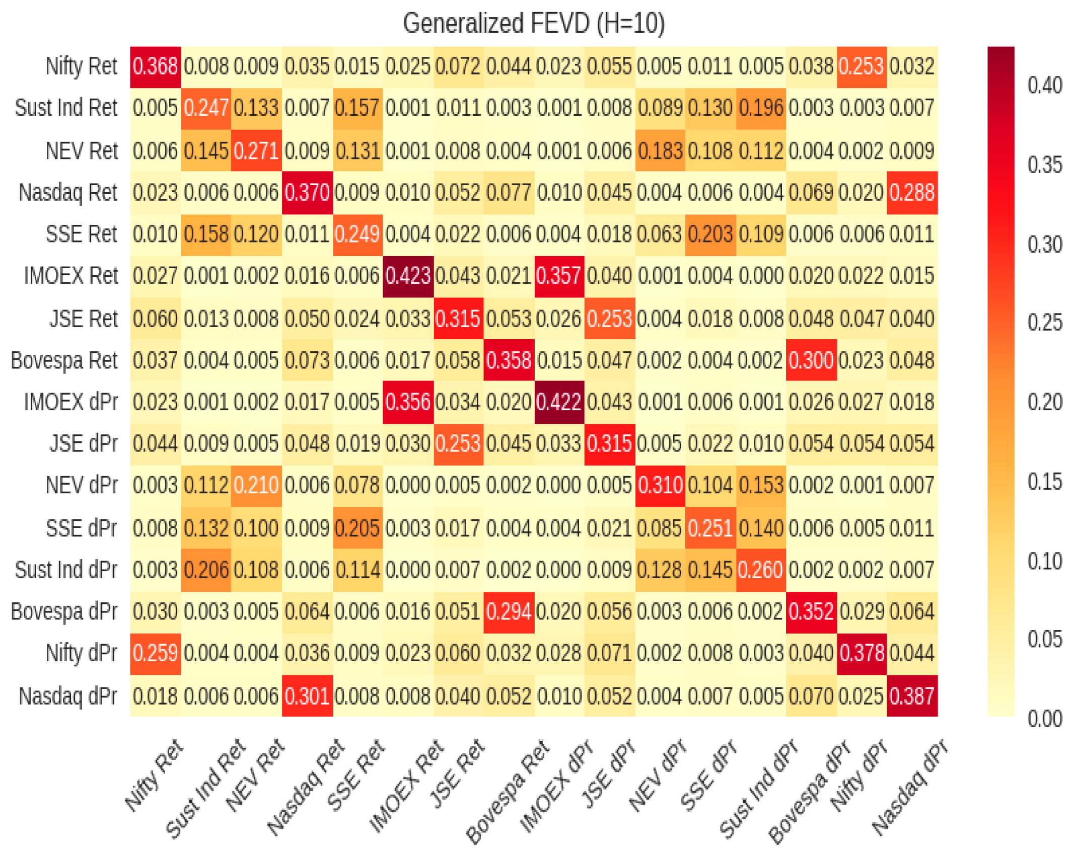
Figure 1. GFEVD matrix.
Risks 13 00222 g001
Figure 2. TCI with structural breaks; BVAR with Minnesota Prior (γ* = 0.1).
Risks 13 00222 g002
Figure 3. Variance breakpoints and segmentations (ΔPrices) (see complete version in Appendix A).
Risks 13 00222 g003
Figure 4. Variance breakpoints and segmentations (returns) (see complete version in Appendix A).
Risks 13 00222 g004aRisks 13 00222 g004b
Figure 5. Impulse response plots (ΔPrices) (see complete version in Appendix A). Note: Event key (referenced in text): 6 July 2018, trade policy shock; 16 March 2020, COVID-19 stress window; 9 November 2020, vaccine news; 24 February 2022, Russia and Ukraine escalation; 7 October 2022, US chip export controls; January 2023, China reopening; 2024–2025, EV sector distress.
Risks 13 00222 g005aRisks 13 00222 g005b
Figure 6. Impulse response plots (returns) (see complete version in Appendix A). Note: Event key (referenced in text): 6 July 2018, trade policy shock; 16 March 2020, COVID-19 stress window; 9 November 2020, vaccine news; 24 February 2022, Russia and Ukraine escalation; 7 October 2022, US chip export controls; January 2023, China reopening; 2024–2025, EV sector distress.
Risks 13 00222 g006aRisks 13 00222 g006b
Figure 7. TCI plot.
Figure 7. TCI plot.
Risks 13 00222 g007
Figure 8. NET (net transmission strength) connectedness plot.
Risks 13 00222 g008
Table 1. Variable description.
Variable NameDescription
Nifty ΔPrNifty 50 Index (ΔPrice)
Nifty RetNifty 50 Index (Returns)
Sust Ind ΔPrSSE Sustainable Industry Index (ΔPrice)
Sust Ind RetSSE Sustainable Industry Index (Returns)
NEV ΔPrSSE New Energy Vehicles Index (ΔPrice)
NEV RetSSE New Energy Vehicles Index (Returns)
Nasdaq ΔPrNasdaq Composite (ΔPrice)
Nasdaq RetNasdaq Composite (Returns)
SSE ΔPrSSE Composite (ΔPrice)
SSE RetSSE Composite (Returns)
IMOEX ΔPrIMOEX Index (ΔPrice)
IMOEX RetIMOEX Index (Returns)
JSE ΔPrFTSE/JSE South Africa Comprehensive (ΔPrice)
JSE RetFTSE/JSE South Africa Comprehensive (Returns)
Bovespa ΔPrBovespa Index (ΔPrice)
Bovespa RetBovespa Index (Returns)
Table 2. Summary statistics and test results.
TestsMeanVarianceSkewnessEx. Kurtosis
Nifty ΔPr8.63425,521.015−0.8498.942
Nifty Ret0.0010.000−1.11221.399
Bovespa ΔPr49.3762,216,707.735−0.86510.643
Bovespa Ret0.0010.000−0.49715.278
IMOEX ΔPr0.6862165.954−5.904132.587
IMOEX Ret0.0000.000−4.137121.413
JSE ΔPr22.162549,543.809−0.2023.573
JSE Ret0.0000.000−0.4167.781
SSE ΔPr−0.0051428.392−0.8269.87
SSE Ret0.0000.000−0.4077.852
Nasdaq ΔPr6.62829,922.818−0.03810.77
Nasdaq Ret0.0010.000−0.1379.795
Sust Ind ΔPr−0.053351.658−0.3385.124
Sust Ind Ret0.0000.000−0.2143.398
NEV ΔPr−0.0372368.14−0.158.698
NEV Ret0.0000.0000.1092.646
Table 3. VAR(1) diagnostics test results.
ModelLag JB Test (p-Value)Ljung–Box Test (p-Value)ARCH-LM Test (p-Value)
ΔPr + Ret 2016–2025100.7206190
500.05470
1000.01420
Table 4. Coefficients of LASSO model.
Variable NETNPT
Nifty ΔPr−8.0715.00
Nifty Ret−8.091.00
Sust Ind ΔPr 3.8712.00
Sust Ind Ret3.9713.00
NEV ΔPr−1.9110.00
NEV Ret−1.6611.00
Nasdaq ΔPr−0.142.00
Nasdaq Ret−2.682.00
SSE ΔPr5.5515.00
SSE Ret5.4314.00
IMOEX ΔPr−1.927.00
IMOEX Ret−2.844.00
Bovespa ΔPr0.565.00
Bovespa Ret−0.695.00
JSE ΔPr6.409.00
JSE Ret2.258.00
Table 5. Chronology of volatility regimes.
Period Important Breaks/TrendsEvents and Causes
2016–2017Overall interconnectedness starts a long-term gradual decrease. A steady downward move in total interconnectedness in 2017.A period of relative stabilization after local crises. Commodity market downsizing. Recession and political instability in Brazil and South Africa. The early anticipation of trade wars.
2018End of a stable regime for Chinese stocks. Interconnectedness stabilizes around 68% after prolapse in 2017.Geopolitical tensions caused by the escalation of the US–China trade wars.
2020A huge, synchronized shock to all the markets. Sharp variance breaks detected across all the indices. TCI peaks at 81.4%.The massive economic and policy uncertainty caused by the global pandemics and associated lockdowns. Coincided with the global dollar squeeze.
2020–2022Post-shock, volatility stabilizes at a significantly higher level than the pre-pandemic period for most markets (Nasdaq, Bovespa).Persistent high volatility due to ongoing pandemic, supply chain disruptions, and shifting economic policies. The regime shift in 2022 coincides with Chinese industrial policy recalibration and U.S. tariff announcements.
2022 Shift to a lower volatility regime for NEV; spillover patterns from Sustainable Industry index change directions. Market maturation, policy changes, and potential reassessment of green sector’s growth valuations after a boom period.
2023Total interconnectedness reaches its lowest point (62.5%).Market divergency due to divergent economic and political policies.
2024–2025A moderate upward move.Geopolitical and climate uncertainty.
Disclaimer/Publisher’s Note: The statements, opinions and data contained in all publications are solely those of the individual author(s) and contributor(s) and not of MDPI and/or the editor(s). MDPI and/or the editor(s) disclaim responsibility for any injury to people or property resulting from any ideas, methods, instructions or products referred to in the content.