Abstract
In this paper, we provide empirical evidence of the market price of risk for delivery periods (MPDP) of electricity swap contracts. The MPDP enables an accurate pricing of such contracts in the presence of the delivery period such that the typical approximations can be avoided. In our empirical study, we focus on term-structure effects and identify the resulting MPDP. In presence of the Samuelson effect, we find the most pronounced MPDP close to maturity, while the MPDP disappears proportional to the Samuelson effect far away from maturity. Thus, our theory improves the pricing accuracy close to maturity.
Keywords:
electricity swaps; delivery period; MPDP for diffusion risk; mean reversion; Samuelson effect JEL Classification:
G130; Q400
1. Introduction
The recent geopolitical tensions make it clear how important adequate risk management of electricity price risk is. Basic risk management tools are futures and options on the futures. Indeed, a large proportion of electricity is traded via future (or swap) contracts, that deliver the electricity over a specified period like a month, a quarter, or a year.1 The delivery period has to be incorporated into the pricing model. In the geometric case, this can induce technical difficulties, and approximations have to be made. The theory of the market price of risk for delivery periods (MPDP), introduced by Kemper et al. (2022) and Kemper and Schmeck (2023), constitutes an elegant method of exact pricing. This paper provides empirical evidence for the existence of the MPDP, constituting a precise pricing framework for futures and options on electricity.
One may say that the starting point of our analysis is the existence of the delivery period in electricity markets. The futures, that are traded, e.g., at the European Electricity Exchange (EEX), typically deliver the underlying electricity over a period of time, in exchange for a fixed futures price. In this paper, we refer to these contracts with delivery periods as swaps. In contrast, we refer to contracts with one time delivery as futures. These contracts are not traded at the exchanges, but are nevertheless useful for constructive purposes: the electricity swap price can be defined as the average with respect to the delivery time of an instantaneous stream of (artificial) futures. This approach is in the spirit of the Heath–Jarrow–Morton approach (see Heath et al. 1990) and has been applied to energy markets by, e.g., Clewlow and Strickland (1999) and Bjerksund et al. (2010).
The problems with the delivery period in geometric models start when averaging arithmetically over the delivery period. The resulting swap price dynamic is neither geometric nor Markovian, due to a complex expression of the volatility term, and therefore of very limited use for further analysis. For a detailed description of the problem, we refer to Kemper et al. (2022) and the references therein. A solution to the problem is the approximation of the swaps volatility coefficient by the average of the futures volatility coefficient, as suggested by Bjerksund et al. (2010). This results in a geometric, Markovian dynamic. It is clear that any approximation always gives rise to an approximation error. Kemper et al. (2022) and Kemper and Schmeck (2023) offer a tractable framework to avoid such approximation errors and allow for precise pricing. They suggest using geometric averaging instead of arithmetic averaging. In a geometric price model as we consider it here, this corresponds to an arithmetic averaging of the drift and volatility coefficients. Indeed, the dynamics are again geometric as well as Markovian. Kemper and Schmeck (2023) discuss the similarities and differences between the approaches of Bjerksund et al. (2010) and Kemper et al. (2022) and introduce a numéraire caused by the different averaging techniques.
Kemper et al. (2022) start with a stream of instantaneous futures contracts that are martingales under some pricing measure . Incorporating the delivery period by geometric averaging does not maintain the martingale property. Therefore, they define the market price of risk for delivery periods that lead to an equivalent measure , that is a martingale measure for the geometrically averaged swap price dynamics.
The new pricing measure will differ from if the volatility of the futures exhibits delivery-dependent effects as, e.g., the Samuelson effect (see Samuelson 1965). The Samuelson effect is typically observed in energy and commodity markets (see, e.g., Benth and Paraschiv 2016; Jaeck and Lautier 2016) and states that there will be an exponential increase in volatility if we come close to the maturity of the contract. In the empirical study presented herein, we focus on the MPDP that is induced by the Samuelson effect.
An additional property of the electricity swap market is the mean-reverting behavior observed under the physical measure . As mentioned by Latini et al. (2019) and Kleisinger-Yu et al. (2020), among others, mean reversion is an important property of electricity swap prices. Koekebakker and Ollmar (2005) empirically validate that the short-term price varies around the long-term price, which confirms mean-reverting behavior. As Benth et al. (2019), we face the problem of changing from the risk-neutral measure to a mean-reverting process of the Ornstein–Uhlenbeck type. We adjust their measure change to our multi-dimensional geometric setting. Figure 1 gives an overview over the measure changes that are involved in our analysis.

Figure 1.
Measure changes between the artificial risk-neutral measure , the swap’s pricing measure , and the physical measure , as well as their connections with the MPDP and the true market price of risk .
In our empirical analysis, we investigate twelve swap contracts with monthly delivery from January to December 2019 traded at the European Electricity Exchange (EEX). That is, here we concentrate on monthly delivering swap contracts exclusively and refer to Kemper et al. (2022) and Piccirilli et al. (2021) for further insights on overlapping swap contracts such as quarterly or yearly swaps.
We put our focus on the analysis of the forthcoming swap contract only, for two reasons. In electricity futures markets, the forthcoming futures is the most liquid one that is traded the most. Furthermore, we concentrate on delivery-dependent effects such as the Samuelson effect, that comes into play when approaching the beginning of the delivery period. Taking these two important aspects together, we have decided to focus on the time horizon of one month for each contract. This could be seen as a relatively short period. Nevertheless, it is only during this short period of time where it is possible to observe the effects that we are looking for. A longer time period does not necessarily improve the quality of the results that we have in mind, that is the MPDP induced by the Samuelson effect.
We fit a model indicating mean-reversion and term-structure effects in the volatility coefficient. The parameters are estimated by maximum likelihood estimation (MLE). The objective of our analysis is to provide evidence for the MPDP, but not to perform an exhaustive empirical study of swap price modeling. Note that we do not perform a term-structure fit by estimating all swap prices occurring at a fixed day since the presence of parallel contracts is limited.
In addition to mean-reversion and term-structure effects, delivery-dependent seasonal effects are observed in electricity markets. Fanelli and Schmeck (2019) empirically identify seasonalities in the swap’s delivery period by considering implied volatilities of electricity options. This feature has an effect on the MPDP as well, which is investigated by Kemper et al. (2022). To analyze the seasonality effects on the MPDP requires, however, a large set of available time series over several years. For this reason, we focus on the influence of the Samuelson term-structure effect on the MPDP exclusively.
Our main contribution to the literature is to show that our geometric averaging approach, leading to the market price of risk for delivery periods, is indeed of importance in practice. That is, we aim at showing empirically that the market price of risk for delivery periods is present in our dataset. For this, we first have to specify our model of Kemper et al. (2022) and Kemper and Schmeck (2023) in a multi-dimensional setting, as we fit several swap price dynamics simultaneously.
The paper is organized as follows: Section 2 presents the geometric averaging approach under the artificial risk-neutral measure applied to the multi-dimensional futures curve. In addition, it presents the MPDP of diffusion risk in order to adjust to the swap’s true risk-neutral measure. Moreover, we introduce the model under the physical measure as a preparation for our empirical study. The estimation procedure and the empirical findings are presented in Section 3. Finally, Section 4 concludes our main findings.
2. The Model and the MPDP
In electricity markets, typically several swap contracts are tradable at the same time, endowed with different delivery periods. For example, at the EEX, the next 9 months, 11 quarters, and 6 years are available. For the scope of this paper, we concentrate on monthly delivering swap contracts.
Let us consider a market with M available swap contracts. The swap contract delivers 1 MWh of electricity during the agreed delivery month, embracing the period from until for . At a trading day before the contract expires, we denote the swap price by , settled such that the contract is entered at no cost. It can be interpreted as an average price of instantaneous delivery. Trading takes place until .
We consider M artificial futures contracts with an —dimensional price . Each component , stands for instantaneous delivery at time . Note that such a contract does not exist on the market but it turns out to be useful for modeling purposes when considering delivery periods (see, e.g., Benth et al. (2019) and Kemper et al. (2022)).
Consider a filtered probability space , where the filtration satisfies the usual conditions. At time , let the price of the artificial futures contracts follow a geometric diffusion process evolving as
where each component of can be characterized by the dynamics of a representative futures price given by
with initial conditions and where W is an —dimensional Brownian motion under with independent components . Furthermore, we assume that is zero if and also if . In this way, we freeze contract m if the time has reached the period of potential delivery and if a point of delivery is considered that is not in the delivery period of contract m.
Remark 1.
In the empirical analysis to come, we concentrate on the last trading month before maturity. Moreover, we focus on monthly contracts that do not overlap. Therefore, each contracting period is characterized by an individual Brownian motion.
We assume that the future price volatility, , depends on both trading time t and delivery time . This enables us to include the Samuelson effect as follows,
such that the futures price volatility is described by a deterministic exponential function with exponential damping factor and a final volatility value that is reached in the end of maturity. This effect goes back to Samuelson (1965) and was implemented in commodity markets, for example, by Schneider and Tavin (2018) and Ladokhin et al. (2024). In addition, it is a typical feature of the electricity market, involving a more pronounced volatility closer to the end of the maturity. Benth and Paraschiv (2016) and Jaeck and Lautier (2016) provide empirical evidence for the Samuelson effect in the volatility term structure of electricity swaps. It can also be observed in the implied volatilities of electricity options, especially far out and in the money (see Kiesel et al. 2009).
Lemma 1
(The Artificial Futures Price under ). The artificial futures price is a -martingale. The unique solution to Equation (2) is given by
Proof.
We know that the volatility from Equation (3) is positive and deterministic as for all m so that suitable integrability and measurability conditions are satisfied. Hence, following Øksendal and Sulem (2007) (cf. Theorem 1.19) there exists a unique solution to Equation (2) given by Equation (4), which follows from the usual procedure. Moreover, from Øksendal and Sulem (2007) (cf. Theorem 1.17), it follows that is a true martingale under . □
Following Heath et al. (1990), we derive the electricity swap price from the artificial futures price as a next step: In order to characterize the electricity swap price appropriately, the implementation of the delivery period plays a crucial role. In particular, the swap price results from averaging an instantaneous stream of artificial futures with respect to the delivery period using a general weight function: where is the corresponding settlement function at . We will follow the most popular example given by a constant settlement type for all such that
This corresponds to a one-time settlement that is independent of the instantaneous settlement time . For a characterization of a continuous settlement, we refer the interested reader to Benth et al. (2008).
To simplify notation, we use the following representation whenever we average over the delivery period:
for some function f and a random variable being uniformly distributed over the delivery period. Furthermore, denotes the variance of a random variable X.
Traditionally, arithmetic weighted averaging is implemented to price swaps in electricity markets (see, e.g., Benth et al. (2008), Bjerksund et al. (2010), and Benth et al. (2019)). However, since the arithmetic average is tailored for arithmetic models, it requires an approximation whenever it is applied to geometric models and whenever we are seeking for explicit solutions. The approximation was first introduced by Bjerksund et al. (2010) in the setting of the electricity market. In order to distinguish between the averaging methods, Kemper and Schmeck (2023) call it the approximated average, leading to a swap price that we denote by . Hence, a representative swap price based on the approximated averaging procedure is defined by
In order to avoid any kind of approximations, Kemper et al. (2022) suggest the use of the geometric average customized for geometric models (see also Kemna and Vorst 1990). The swap price based on geometric averaging will be denoted by F. Hence, a representative swap price based on the geometric averaging procedure is defined by
In a next step, we characterize both versions of representative electricity swaps in Equations (6) and (7), in order to investigate the consequences of the often-used approximation procedure.
Lemma 2.
Under the artificial pricing measure , the dynamics of a representative swap price based on approximated averaging procedure are given by
Proof.
Since the volatility is deterministic, measurable, and , we can show that
so that we can apply the stochastic Fubini Theorem (see Protter (2005), cf. Theorem 65, Chapter IV. 6), which gives Equation (8). □
Definition 1
(Swap Price Volatility). We define the swap price volatility by
which is the average futures price volatility over the delivery period with density .
Remark 2.
Note that the swap price volatility simplifies to
for a constant parameter such that the swap price volatility still preserves the Samuelson effect until maturity .
Note that actually depends on the length of the delivery period as it is precisely denoted in Kemper et al. (2022) (by choosing the notation ). For simplicity we skip this dependence as we consider only monthly delivery periods in the empirical analysis to come.
In contrast, geometric averaging originates from the arithmetic average of logarithmic returns without any need for approximations. Hence, in line with Kemper et al. (2022), we define the swap price originating from geometric averaging as follows.
Lemma 3
(Swap under ). Under the artificial pricing measure , the dynamics of a representative swap price based on the geometric averaging procedure is given by
where U denotes the random delivery variable with density and .
Proof.
We summarize all swap prices that are available during the trading horizon as an —dimensional process given by
where is an —dimensional Brownian motion and is an —dimensional deterministic drift vector.
Although the futures prices and the approximated swaps are martingales under the pricing measure , the swap price F is not a -martingale: It turns out, that the resulting swap price dynamics is a geometric process endowed with the same swap price volatility as in Lemma 2. However, note that in general the swap price dynamics in Equations (8) and (12) do not coincide, due to a non-zero drift term arising in Equation (12). More precisely, the swap price process F under has a negative drift term characterized by the swap’s variance.
Remark 3
(Swap Price Drift under ). We can simplify the drift term of the representative swap price to
for a constant parameter such that the swap’s drift also preserves a squared Samuelson effect until maturity . Note that again depends on the length of the delivery period, which will be skipped for notational convenience.
Hence, using geometric averaging leads to a new interpretation of risk related to the delivery period going along with an adjustment of the swap’s risk-neutral measure that we denote by .
As introduced by Kemper et al. (2022), the gap between the classical risk-neutral measure and the swap’s true risk-neutral measure is characterized by the MPDP, which we define in the following:
Definition 2
(The MPDP). At time , the market price of diffusion risk for delivery periods associated with all equidistant delivery periods for is defined by , where
Remark 4.
Using the notation above, the MPDP for a representative swap contract simplifies to
such that the MPDP preserves the Samuelson effect until maturity .
In particular, refers to the additional diffusion risk associated with each available swap contract. Note that the MPDP of diffusion risk, , is negative. Hence, the geometric averaging technique induces less risk than the application of the approximated arithmetic average, for which we need to pay a cost of approximation risk. Vice versa, using the geometric average induces less risk than the approximated arithmetic one such that the overall risk is lowered. Consequently, risk is reduced whenever the correct, and thus non-approximated, averaging procedure is implemented. It can be interpreted as the trade-off between the weighted average variance of a stream of futures, on the one hand, and the variance of the swap, on the other hand. Note that the MPDP of a representative swap, , is in line with the MPDP for diffusion risk found in Kemper et al. (2022), where a stochastic volatility scenario is considered.
In Equation (17), we can clearly observe that the MPDP preserves the term-structure effect: The MPDP splits into a negative constant, characterized by the Samuelson parameter and the length of the delivery period , and the deterministic exponential term-structure effect. Hence, the MPDP becomes more pronounced closer to the end of maturity.
Note, if in the exceptional case that the future price volatility is independent of the delivery time, then both swap prices in Lemmas 2 and 3 directly coincide. Moreover, they are martingales under since the MPDP in Equation (16) is zero whenever delivery dependence fails to appear.
We define a new pricing measure such that the —dimensional swap price processes are martingales. Following Øksendal and Sulem (2007), define the Radon–Nikodym density through
Assume that is a martingale for the entire trading time. We then define the new measure through the Radon–Nikodym density
which clearly depends on all delivery periods .
Hence, a straightforward valuation leads to the following result.
Proposition 1
(Swap under ). The swap price process , defined in (14), is a martingale under . The corresponding dynamics are given by
where is an —dimensional Brownian motion under , defined through
during the trading horizon .
Proof.
We know by definition that is a continuous deterministic process that is square-integrable since
Hence, all processes are adapted. Following Øksendal and Sulem (2007) (cf. Theorem 1.35), we need to show that , defined in Equation (18), is a true martingale. Since are independent of each other, it is enough to show, that
for are true martingales. We can prove Novikov’s condition (see, e.g., Protter 2005, cf. Theorem 41, Chapter III.8) as satisfies
Hence, for all m, and so , are true martingales. Hence, we can apply Girsanov’s Theorem (see, e.g., Øksendal and Sulem 2007, cf. Theorem 1.35) and the assertion follows. □
In order to investigate the model empirically, we introduce the model under its physical measure . A typical drift feature is the mean-reverting behavior (see, e.g., Benth et al. (2008) and Benth et al. (2019)), which we implement at the swap’s rate level following Kemper and Schmeck (2023).
Lemma 4
(Swap under ). Under the physical measure , the representative swap price process, , evolves as
We find that are independent Brownian motions under the physical measure , characterized by
where the true market price of risk, , is defined through
Proof.
Analogous to Kemper and Schmeck (2023) (Section 2.2 and Appendix B) and to Benth et al. (2019) (Theorem 3.5 and Appendix B), where both references are dealing with one-dimensional swap price dynamics, either with jumps and stochastic volatility or jumps exclusively. The proof in the multi-dimensional setting can be found in Appendix A. □
Remark 5.
- (i)
- The logarithmic price of a representative swap contract evolves asThe solution is given byHence, we observe that the mean-reverting behavior enters as a modified second term-structure effect. The Samuelson effect is exclusively present in the volatility term and strengthens the speed of mean reversion.
- (ii)
- Note, that the swap’s logarithmic returns are based on logarithmic future price returns defined by
In order to discretize the model of Lemma 4 under the physical measure , we follow the Euler-type discretization procedure with step size . The discretized logarithmic price of the swap from Equation (27) is denoted by , with , and is given by the following Lemma.
Lemma 5.
The discretized logarithmic price of a representative swap price
for and is a standard normal-distributed random variable. Moreover, the coefficients to be estimated are , where , and , with and where we denote as the length of the time series with delivery during .
Hence, the likelihood of our discretized model in Lemma 5 can be expressed in terms of the conditional probability density function
where is the set of parameters, and determines the conditional probability density function for contract m at data point j. In particular, such that the conditional probability density function is given by
where the set of parameter values is subject to , and .
We recalibrate the parameters to characterize , and accordingly:
Remark 6.
By construction, the contracts are independent of each other. We justify this assumption since we only fit the last—most liquid—trading month of the contracts and the contracts do not overlap.
3. Empirical Analysis
In this section, we provide empirical evidence for the MPDP of monthly electricity swap contracts. We base our analysis on the discretized model introduced in Lemma 5 and estimate the model’s parameter values by maximum likelihood estimation (MLE) with respect to the dataset that is presented in Section 3.1. The results of our empirical analysis are presented in Section 3.2. You can find a discussion on the empirically identified MPDP in Section 3.4.
3.1. Description of the Dataset
We consider twelve electricity swap contracts with monthly delivery periods in 2019 traded at EEX. In particular, we work with the time series of the Phelix Base Monthly Energy Futures2 from 3 December 2018 to 29 November 2019, covering the last trading month before maturity that does not overlap with other contracts. We use weekday prices to exclude weekend effects so that we investigate on average about 21 data points before the contract expires. This might not seem to be a large sample; nevertheless, remember that we focus on delivery-dependent effects that appear only a short time before the delivery of the contract. A larger sample with more data points far away from delivery would not necessarily improve the quality of the results.
We provide an overview over the general characteristics of each electricity swap contract in Table 1, including the start and maturity of the considered time series, the range of the considered trading time, the amount of investigated data points, the minimum, maximum, average prices, and the average standard deviation. The average number of trading days within the last trading month is around 21 days. The average prices are highest in January and February. The standard deviations computed over all monthly contracts range from 0.83576 to 3.0682, appearing highest in the first quarter of the year and in May. The May swap contract, however, has to be treated carefully since the time series is not completely available to us as the last data point already lies in the middle of April, and thus it covers 10 available data points only.

Table 1.
General characteristics of the Phelix Base Monthly Energy Futures dataset.
Figure 2 depicts the time series of prices and logarithmic returns for each swap contract with respect to time to maturity measured in days. The prices in Figure 2a can be categorized at a high level, around 60 €/MWh—for January and February—and a lower level, between 35.38 and 47.38 €/MWh, for the remaining contracts. On average, the prices turn slightly downwards until the end of maturity is reached. The logarithmic returns in Figure 2b are usually located between values of −0.04 and 0.04, with some outliers that are largest close to the end of maturity.
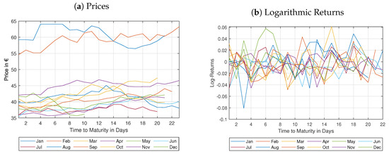
Figure 2.
Time series for prices and logarithmic returns of all monthly electricity swap contracts maturing in 2019 plotted with respect to time to maturity during the last trading month.
For this reason, we formally test the swap’s logarithmic returns on normality using Matlab’s Jarque–Bera test jbtest for the considered time horizon. The test returns a decision for the null hypothesis that the data come from a normal distribution with significant p-values for most of the contracts. We summarize our test results in Table 2, where 0 indicates a failure to reject the null hypothesis of normally distributed logarithmic returns at a significance level of 0.05. It turns out that all swap contracts accept the normal hypothesis. This validates our assumption that jumps are absent during the last trading month or smoothed out in a swap contract by averaging over the delivery period.
Table 2.
Test results for normality and mean reversion at a significance level of 0.05. (Jarque-Bera test h = 1 indicates rejection of normal distribution. adftest h = 1 indicates an AR(1) model with drift coefficient.) Note that the adftest returns minimum (0.001) or maximum (0.999) p-values if the test statistics are outside the tabulated critical values, where *** indicates a significance level below 0.1%, ** a significance level below 1%, and * below 5%.
In order to verify our model choice, we additionally test the mean-reverting behavior using the augmented Dickey–Fuller (ADF) test adftest for autocorrelation. The ADF test is designed to detect the presence of a unit root, rather than serial correlation. The null hypothesis of the ADF test is the presence of a unit root. The value 1 indicates mean-reverting effects appearing whenever the p-value is below the significance level 0.05. Indeed, except for May, all swap contracts reject the null hypothesis so that mean-reverting behavior is clearly present. As mentioned before, the May contract has to be treated carefully due to the short available trading horizon within the last trading month. Thus, this “May effect” could be a data-related issue. Hence, our results might also confirm our choice of mean-reverting logarithmic returns. Nevertheless, we double check the presence of mean-reverting effects by evaluating the goodness of fit at the end of the next subsection. First of all, however, we move on to the results of the estimation procedure.
3.2. Empirical Results
We now present the results of the empirical analysis of the swap price data considered in Section 3.1. We fit the logarithmic prices using the MLE technique to obtain the parameter estimates by maximizing the likelihood in Equation (31) with respect to the parameter set . The optimization procedure is implemented in Matlab using the simulannealbnd function based on simulated annealing (see Goffe et al. (1994), also used by Schneider and Tavin (2018)). For each contract, we fit the logarithmic swap prices by maximizing the likelihood in (31). According to Equation (32), we recalibrate the parameter estimates and summarize the transformed parameter values in Table 3. Note that even if the data might be not Gaussian, the use of the maximum likelihood estimator can still be justified as a quasi-maximum likelihood estimator. Following White (1982), the variance–covariance matrix of the estimators needs to be adjusted in such a case.
Table 3.
Recalibrated model parameter estimates with corresponding p-values, where *** indicates a significance level below 0.1%, ** a significance level below 1%, and * below 5%.
In Table 3, we list the recalibrated model parameters per contract and their corresponding coefficients according to the transformation in (32). The transformation leads to a mean-reversion level that is—except for January, May, July, and August—negative: It is the smallest in March at −2.8479 and on average around −0.41989, as we have already observed in Figure 2. The highest values can be found in January, May, July, and August, with values between 1.121 in January and 4.3179 in May. One possible explanation for this observation might be the uncertainty regarding the availability of electricity, especially for seasons with a high electricity intensity due to heating or air conditioning. We observe that the speed of mean reversion is very high, so that the half life lies within one day. The p-values of the parameter estimates are significant for most of the contracts. We remark that the data in May are to be treated with care as some data are missing.
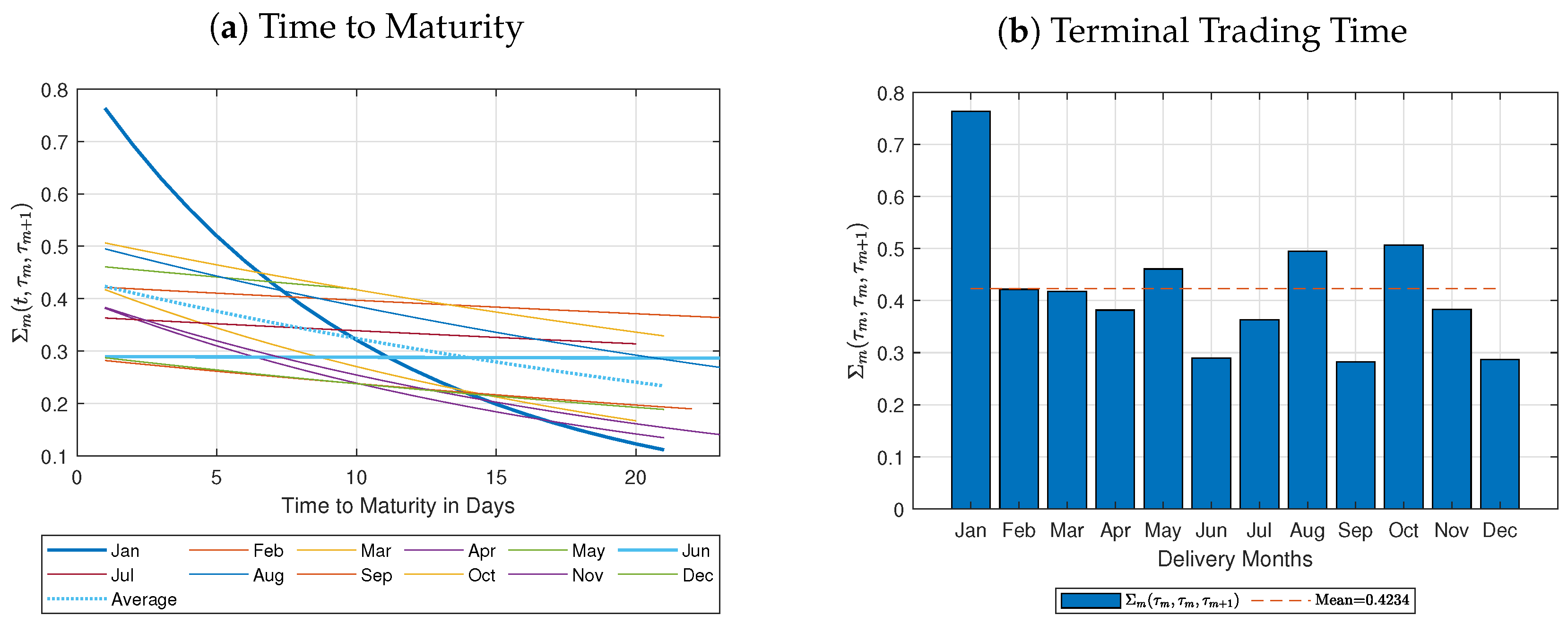
Moreover, we observe that the average volatility is around 0.43617, ranging from around 0.28958 in June to 0.84019 in January. The average volatility is dampened by the Samuelson effect. Note that the Samuelson parameter is smallest in June and highest in January, connected with a relatively low and very high average volatility, respectively. This combination leads to a very pronounced Samuelson effect in January, visualized in Figure 3a, highlighted with a bold blue. The contrary happens for the smallest Samuelson parameter, in June, for which the volatility appears to be a straight line, in bold light blue.

Figure 3.
Volatility function with Samuelson effect. (a) Volatility over time to maturity. (b) Volatility at terminal trading time.
More precisely, the swaps volatility is visualized in Figure 3 for each contract over the considered time to maturity. As mentioned before, the most pronounced effect can be found in January and the least pronounced effect appears in June. In most of the contracts, we clearly observe the term-structure effect induced by the swaps volatility (see Definition 1): The closer we reach to the end of the maturity, the more effect the volatility has. The average Samuelson effect is highlighted by a dotted line for a time horizon of 21 days before maturity, which is the average number of trading days within the last trading month (see also Table 1). The average Samuelson effect starts at 0.2336 and reaches 0.4234 at the end of the maturity, driven by the average Samuelson parameter 7.4944 (see Table 3). For comparative reasons, we depict the terminal values of the swaps volatility in Figure 3b for each contract. The average terminal value is around 0.4234; it is exceeded by the swap contracts maturing in January, May, August, and October.
3.3. On the Goodness of Fit
In Section 3.1, we have already tested the presence of mean reversion. Except for the swap contract in May, all time series indicate mean-reverting behavior. To double check this feature, we compare our investigated model to the case without mean reversion by choosing for all . We particularly consider the relative and absolute goodness of fit of our model in Lemma 5 with and without mean reversion. For this comparison, we rely on a procedure applied, e.g., by Zucchini et al. (2021) and Schneider and Tavin (2018).
For the relative goodness of fit, we consider the models’ logarithmic likelihoods (LLHs), their Akaike information criteria (AICs), and the Bayesian information criteria (BICs), described in Table 4. We aim to maximize the likelihood. Hence, the higher the LLH, the better. We observe a higher LLH for the model with mean reversion. Moreover, the best model ideally induces the smallest AIC and BIC, such that a high LLH stands in an adequate relation to the number of parameters. Again, the mean-reverting effects lead to a better result. Hence, the Samuelson model inducing mean-reverting behavior fits better in all criteria.
Table 4.
Relative and absolute goodness of fit.
For the absolute goodness of fit, we consider the deviance and the likelihood ratio test (LRT) described in Table 4. The deviance is zero for the model with the highest likelihood. Consequently, the combination of the Samuelson effect and mean reversion induces a deviance that is zero. The closer the deviance for the remaining model, the better the model. However, it is hard to verify whether the deviance of 12.294 is close or far away from zero for the model without mean reversion. As it is known that the deviance follows a distribution with three parameters in the seasonality-type model, we apply the LRT. The LRT returns the rejection decision and p-value for the hypothesis test conducted at a significance level of 0.05. We observe that the p-value is below this threshold. This indicates strong evidence suggesting that the model with the higher likelihood fits the data better than the model restricted to three parameters only. As a consequence, we can conclude that the combination of the Samuelson effect and mean reversion is the best for both considered models.
3.4. On the MPDP
In Definition 2, we analytically define the MPDP, that is expressed through a constant negative component, , and the continuous Samuelson effect, . Both components can be identified based on the estimated parameter values in Table 3 (see also the definition of in Definition 1 and for in Remark 3).
In Table 5, we provide the coefficients and , with which we can finally derive the constant component of the MPDP . We observe that the constant component is negative and varies between −0.0684 in January and in June. On average, the component is located around −0.01516. It is negative as we reduce risk whenever we avoid the approximation induced by approximated averaging. The closer we come to the end of the maturity, the greater the effect the constant MPDP component has since we multiply it with the continuous Samuelson effect. This continuous component, , has already been addressed in Section 3.2. Note that by Equation (11) we know that
Consequently, the Samuelson effect, and thus the continuous component, is found by rescaling the swaps’ volatility, which has been already visualized in Figure 3a.
Table 5.
Further model coefficients resulting from Table 3, where *** indicates a significance level below 0.1% and * below 5%.
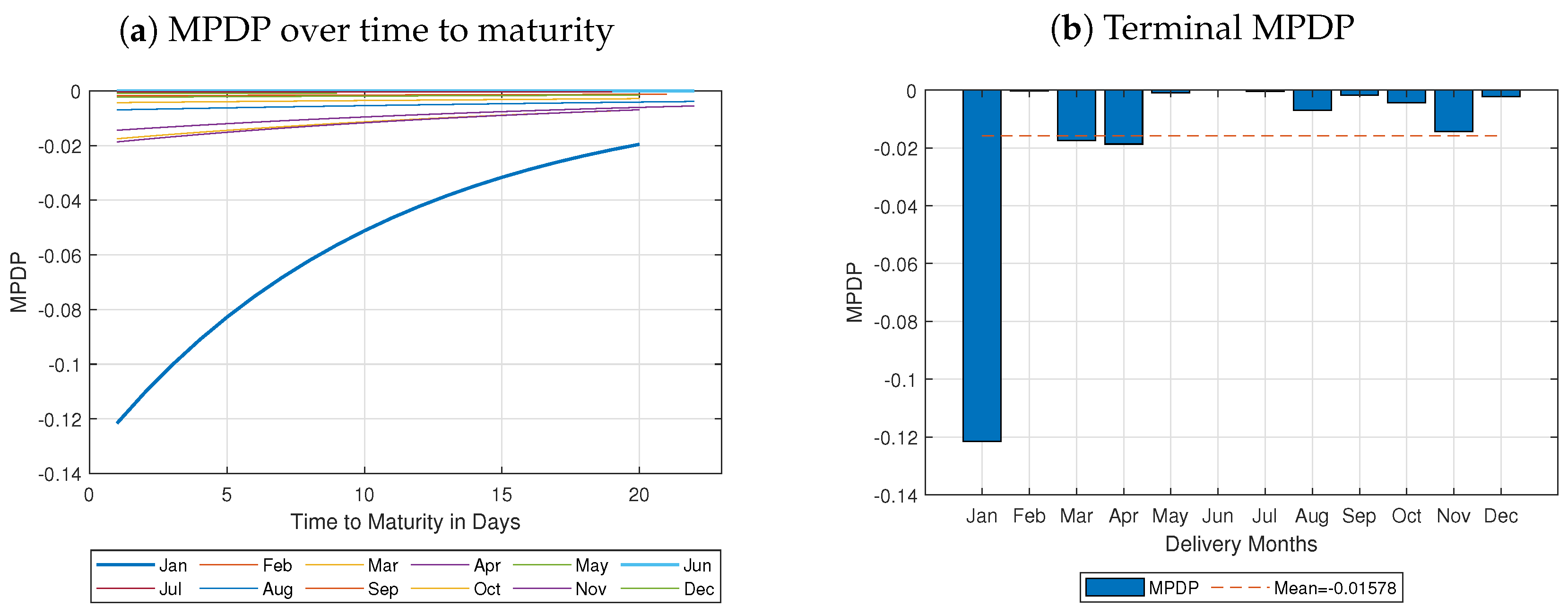
We calculate the MPDP derived in Definition 2 by multiplication of the constant and continuous component. Figure 4a depicts the MPDP for each contract over time to maturity. The MPDP is negative and decreases further the closer we come to the expiration date. Especially for January, the MPDP is highest in terms of the absolute value, up to −0.1216, at the terminal time. For the sake of comparison, we include a barplot of the terminal MPDP in Figure 4b. According to Figure 4b, a delivery dependence in terms of the Samuelson effect is especially visible in January, March, and April. At the terminal time, the average MPDP is found at −0.01578, shown as a dashed line. Since we consider a geometric model, the MPDP can be interpreted as a relative value. Consequently, with the MPDP we can reduce risk by on average.

Figure 4.
MPDP of diffusion risk for all contracts with mean reversion. (a) MPDP over time to maturity. (b) Terminal MPDP.
Note that the behavior of the term structure within the MPDP was first observed by Kemper et al. (2022) numerically using three types of Samuelson parameters complemented by a stochastic volatility setup. We here provide the empirical evidence for the shape of the MPDP, which is even more pronounced since the estimated Samuelson effect is around (see Table 3).
4. Conclusions
In this paper, we provide empirical evidence as well as analytical characteristics of the market price of risk for delivery periods (MPDP) driven by term-structure effects.
We adjust the model of Kemper et al. (2022) to a multi-dimensional model with deterministic volatility. In particular, the volatility includes a term-structure effect known as the Samuelson effect (see Samuelson 1965). This term structure is preserved in the swaps’ volatility. In addition, we compare swap prices resulting from geometric averaging with swaps based on approximated averaging in line with Kemper et al. (2022) and Bjerksund et al. (2010). We identify an approximation gap between swap contracts resulting from approximated and geometric averaging. The distance between their risk-neutral measures, and , characterizes a gap that is defined as the MPDP. As the MPDP leads to the true pricing measure, , the spread remediates the approximated swap price and adjusts it downwards to the correct price of the swap contract. Consequently, any pricing methodology based on approximated averaging can easily be turned to the “correct” risk-neutral measure by an application of our MPDP. In Definition 2, we determine the MPDP analytically. It turns out to be negative and decreasing with time to maturity. Moreover, it preserves the Samuelson effect, which is in line with the findings in Kemper et al. (2022).
In preparation for our empirical analysis, we investigate the model under the physical measure. In particular, we implement mean reversion in the logarithmic returns in the spirit of Benth et al. (2019). Moreover, we provide the resulting discretized swap price model. Empirically, we consider the last trading month of 12 monthly swap contracts delivering in 2019. We fit the discretized model to the logarithmic prices using the MLE procedure. Our empirical results confirm the presence of mean reversion and a short-term Samuelson effect. Based on the parameter estimates, we provide an empirical characterization of the MPDP: The term-structure dependence induces a decreasing behavior of the MPDP over time to maturity. Hence, the closer we come to the expiration date, the more pronounced the MPDP, and the larger the approximation gap. For instance, the MPDP at the terminal time amounts on average to −12.16% for a swap delivering in January 2019. Consequently, the MPDP reduces risk caused by approximated averaging, especially when the end of the maturity approaches.
Indeed, another important feature of the market is seasonalities in the delivery period: Fanelli and Schmeck (2019) empirically identify those seasonalities by considering implied volatilities of electricity options. Moreover, Kemper et al. (2022) investigate the MPDP analytically regarding seasonalities in the delivery period. Varying weather conditions over the seasons of a year might cause even stronger delivery-dependent behavior when the share of renewables is growing. In this case, we even expect a growing MPDP caused by a rising market share of renewable energy since they strongly depend on the weather conditions of the season. Consequently, this increases the importance of the MPDP, which has to be taken into account to ensure an accurate pricing procedure. It might be very interesting to investigate this phenomenon and the MPDP driven by seasonalities empirically. This, however, is a question for future research.
Author Contributions
Conceptualization, M.D.S.; Methodology, A.K. and M.D.S.; Formal analysis, A.K.; Investigation, A.K.; Data curation, A.K.; Writing—original draft, A.K. and M.D.S.; Supervision, M.D.S.; Writing—review and editing, A.K. and M.D.S. All authors have read and agreed to the published version of the manuscript.
Funding
This research was funded by Deutsche Forschungsgemeinschaft (DFG, German Research Foundation) grant number SFB 1283/2 2021-317210226.
Data Availability Statement
The data that support the findings of this study are available from the corresponding author, A. Kemper, upon reasonable request. The data are not publicly available due to privacy restrictions.
Conflicts of Interest
No potential competing interest was reported by the authors.
Appendix A. Proof of Lemma 4
Following Øksendal and Sulem (2007), we define the Radon–Nikodym density through
where the market price of risk, , is defined in Equation (26). Inspired by Benth et al. (2019), we prove that and adjust their Theorem 3.5 to our multi-dimensional geometric jump-free setting with independent Brownian motions. Moreover, instead of turning from the physical measure to the risk-neutral measure, we start from the swaps’ true martingale measure .
We proceed in the following steps using the notation :
- Derivation of a new physical measure through a stopping time .
- Proof that is lower-bounded by .
- Proof that there exists an upper boundary for for all contracts .
1. Derivation of . Similar to Benth et al. (2019), we define the adapted compensator of by , where . Note that this multi-dimensional setting covers an —dimensional market price of risk for all independent random parts .
Now, let us define a sequence of stopping times depending on the random part of the market price of risk:
Observe that for every , the stopped process is bounded. Hence, by Lépingle and Mémin (1978) (cf. Theorem III.1), we know that for , and so is a uniformly integrable martingale such that we can define the probability measure by
2. Proof of lower boundary of . First, is a positive local martingale. Hence, it is a supermartingale, so that we know the upper boundary for :
Next, we consider the lower boundary, following Benth et al. (2019):
where the last equality follows from the change of measure defined in step 1 (see (A4)). By definition of the stopping time (see (A3)), we deduce
where the last inequality follows from Markov’s inequality. If we show that the expectations on the right-hand side have upper boundaries that are independent of , then , which is addressed in the third step.
3. Proof of upper boundaries. In order to identify upper boundaries under the measure defined in (A4), we need to derive the dynamics of a representative logarithmic swap price under . We therefore apply Girsanov’s theorem (see Øksendal and Sulem 2007, cf. Theorem 1.35), leading to
where are independent Brownian motions under .
Next, we show that is uniformly integrable:
The first equality represents the integral version of Y under . Inequality results from the Cauchy–Schwartz inequality to the sum and an application of the triangle inequality. We apply Doob’s inequality to all expectations in Inequality as well as the upper boundary of the swap’s volatility in Equation (11). In Inequality , we apply the Cauchy–Schwartz inequality to the first three integrals. We finish with Itô–Lévy isometry (see Øksendal and Sulem 2007, cf. Theorem 1.17) to the last summand and an application of the stochastic Fubini theorem to the fourth summand while making the integrand even bigger. By the choice of , an application of Gronwall’s inequality yields , where , such that is indeed a true martingale.
Notes
| 1 | See, e.g., the EEX Group Volume Report from September 2024 at www.eex.com/de/newsroom/detail?tx_news_pi1%5Baction%5D=detail&tx_news_pi1%5Bcontroller%5D=News&tx_news_pi1%5Bnews%5D=12850&cHash=09727e9d7cca9ca342be43788c2b174b (accessed date: 16 December 2024) for further details. |
| 2 | Note that the name Futures refers in our context to swap contracts. |
References
- Benth, Fred Espen, Jūratė Šaltytė Benth, and Steen Koekebakker. 2008. Stochastic Modelling of Electricity and Related Markets. Singapore: World Scientific Publishing Company, vol. 11. [Google Scholar]
- Benth, Fred Espen, and Florentina Paraschiv. 2016. A Structural Model for Electricity Forward Prices. Working Papers on Finance No. 2016/11. St. Gallen: University of St. Gallen. [Google Scholar]
- Benth, Fred Espen, Marco Piccirilli, and Tiziano Vargiolu. 2019. Mean-Reverting Additive Energy Forward Curves in a Heath-Jarrow-Morton Framework. Mathematics and Financial Economics 13: 543–77. [Google Scholar] [CrossRef]
- Bjerksund, Petter, Heine Rasmussen, and Gunnar Stensland. 2010. Valuation and Risk Management in the Norwegian Electricity Market. In Energy, Natural Resources and Environmental Economics. Edited by Endre Bjørndal, Mette Bjørnda, Panos M. Pardalos and Mikael Rönnqvist. Berlin and Heidelberg: Springer, pp. 167–85. [Google Scholar]
- Clewlow, Les, and Chris Strickland. 1999. Valuing Energy Options in a One Factor Model fitted to Forward Prices. Research Paper Series, No 10. Sydney: Quantitative Finance Research Centre, University of Technology. [Google Scholar]
- Fanelli, Viviana, and Maren Diane Schmeck. 2019. On the Seasonality in the Implied Volatility of Electricity Options. Quantitative Finance 19: 1321–37. [Google Scholar] [CrossRef]
- Goffe, William L., Gary D. Ferrier, and John Rogers. 1994. Global Optimization of Statistical Functions with Simulated Annealing. Journal of Econometrics 60: 65–99. [Google Scholar] [CrossRef]
- Heath, David, Robert Jarrow, and Andrew Morton. 1990. Bond Pricing and the Term Structure of Interest Rates: A New Methodology for Contingent Claims Valuation. Econometrica 60: 77–105. [Google Scholar] [CrossRef]
- Jaeck, Edouard, and Delphine Lautier. 2016. Volatility in Electricity Derivative Markets: The Samuelson Effect Revisited. Energy Economics 59: 300–13. [Google Scholar] [CrossRef]
- Kemna, Angelien G. Z., and Antonius Cornelis Franciscus Vorst. 1990. A Pricing Method for Options based on Average Asset Values. Journal of Banking and Finance 14: 113–29. [Google Scholar] [CrossRef]
- Kemper, Annika, Maren Diane Schmeck, and Anna Khripunova Balci. 2022. The Market Price of Risk for Delivery Periods: Pricing Swaps and Options in Electricity Markets. Energy Economics 113: 106221. [Google Scholar] [CrossRef]
- Kemper, Annika, and Maren Diane Schmeck. 2023. Pricing of Electricity Swaps with Geometric Averaging. arXiv arXiv:2303.12527. [Google Scholar]
- Kiesel, Rüdiger, Gero Schindlmayr, and Reik H. Börger. 2009. A Two-Factor Model for the Electricity Forward Market. Quantitative Finance 9: 279–87. [Google Scholar] [CrossRef]
- Kleisinger-Yu, Xi, Vlatka Komaric, Martin Larsson, and Markus Regez. 2020. A Multifactor Polynomial Framework for Long-Term Electricity Forwards with Delivery Period. SIAM Journal on Financial Mathematics 11: 928–57. [Google Scholar] [CrossRef]
- Koekebakker, Steen, and Fridthjof Ollmar. 2005. Forward Curve Dynamics in the Nordic Electricity Market. Managerial Finance 31: 73–94. [Google Scholar] [CrossRef]
- Ladokhin, Sergiy, Maren Diane Schmeck, and Svetlana Borovkova. 2024. From Calender Time to Business Time: The Case of Commodity Markets. International Journal of Theoretical and Applied Finance 27: 2450018. [Google Scholar] [CrossRef]
- Latini, Luca, Marco Piccirilli, and Tiziano Vargiolu. 2019. Mean-reverting No-arbitrage Additive Models for Forward Curves in Energy Markets. Energy Economics 79: 157–70. [Google Scholar] [CrossRef]
- Lépingle, Dominique, and Jean Mémin. 1978. Sur l’intégrabilité Uniforme des Martingales Exponentielles. Zeitschrift für Wahrscheinlichkeitstheorie und verwandte Gebiete 42: 175–203. [Google Scholar] [CrossRef]
- Øksendal, Bernt, and Agnès Sulem. 2007. Applied Stochastic Control of Jump Diffusions. Cham: Springer. [Google Scholar]
- Piccirilli, Marco, Maren Diane Schmeck, and Tiziano Vargiolu. 2021. Capturing the Power Options Smile by an Additive Two-factor Model for Overlapping Futures Prices. Energy Economics 95: 105006. [Google Scholar] [CrossRef]
- Protter, Philip E. 2005. Stochastic Differential Equations. In Stochastic Integration and Differential Equations. Stochastic Modelling and Applied Probability. Berlin/Heidelberg: Springer, vol. 21. [Google Scholar]
- Samuelson, Paul A. 1965. Proof that Properly Anticipated Prices Fluctuate Randomly. Industrial Management Review 6: 41–49. [Google Scholar]
- Schneider, Lorenz, and Bertrand Tavin. 2018. From the Samuelson Volatility Effect to a Samuelson Correlation Effect: An Analysis of Crude Oil Calendar Spread Options. Journal of Banking and Finance 95: 185–202. [Google Scholar] [CrossRef]
- White, Halbert. 1982. Maximum Likelihood Estimation of Misspecified Models. Econometrica 50: 1–25. [Google Scholar] [CrossRef]
- Zucchini, Walter, Ian L. MacDonald, and Roland Langrock. 2021. Hidden Markov Models for Time Series: An Introduction Using R, 2nd ed. New York: Chapman and Hall. [Google Scholar]


Disclaimer/Publisher’s Note: The statements, opinions and data contained in all publications are solely those of the individual author(s) and contributor(s) and not of MDPI and/or the editor(s). MDPI and/or the editor(s) disclaim responsibility for any injury to people or property resulting from any ideas, methods, instructions or products referred to in the content. |
© 2025 by the authors. Licensee MDPI, Basel, Switzerland. This article is an open access article distributed under the terms and conditions of the Creative Commons Attribution (CC BY) license (https://creativecommons.org/licenses/by/4.0/).