A Note on a Modified Parisian Ruin Concept

Abstract

Traditionally, Parisian ruin is said to occur when the insurer’s surplus process has stayed below level zero continuously for a certain grace period. Inspired by this concept, in this paper we propose a modification by assuming that once a grace period has been granted when the surplus becomes negative, the surplus level will not be monitored continuously in the interim, but instead it will be checked at the end of the grace period to see whether the business has recovered. Under an Erlang distributed grace period, a computationally tractable formula for the Gerber–Shiu expected discounted penalty function is derived. Numerical examples regarding the modified Parisian ruin probability are also provided.

1. Introduction

In this paper, the evolution of the insurer’s surplus is modeled by the compound Poisson risk process with dynamics

$$U\left(t\right)=u+ct-\sum _{i=1}^{N\left(t\right)}{Y}_i,t\ge 0,$$

where $u=U\left(0\right)\ge 0$ is the initial surplus, $c>0$ is the premium rate per unit time, ${\left\{N\left(t\right)\right\}}_{t\ge 0}$ is a Poisson process with the rate $\lambda >0$, and ${\left\{Y_i\right\}}_{i=1}^{\infty }$ form a sequence of independent and identically distributed (i.i.d.) claim amounts independent of ${\left\{N\left(t\right)\right\}}_{t\ge 0}$. It is further assumed that $Y_1$ is a positive continuous random variable with density $f_Y$ and Laplace transform ${\tilde{f}}_Y$. The positive security loading (or net profit) condition of the model is $c>\lambda \mathbb{E}\left[Y_1\right]$. In the rest of the paper, we shall use ${\mathbb{P}}_u$ and ${\mathbb{E}}_u$, respectively, to denote the probability and expectation taken under the initial condition $U\left(0\right)=u$.

While the classical ruin time ${\tau }_{\mathrm{CL}}=inf\{t\ge 0:U\left(t\right)<0\}$ (with the convention $inf\varnothing =+\infty$) is defined to be the first time the surplus process falls below zero, the resulting deficit at ruin $\left|U\right({\tau }_{\mathrm{CL}}\left)\right|$ may not be large, and one may argue that it is still worthwhile for the insurer to continue its business as long as it is profitable in the long ruin (so that it will recover with probability one). In the compound Poisson model, Dassios and Wu (2008a, 2008b) first proposed that the Parisian ruin time is defined as the first time when the surplus process has continuously remained negative for a prescribed period $d>0$ granted by the regulator. They derived the exact Laplace transform of the Parisian ruin time for exponential claims and the asymptotic ruin probability for light-tailed claims, and further results in the same model were subsequently obtained by, e.g., Czarna et al. (2017) and Landriault et al. (2019, Section 3.3). The concept of Parisian ruin was indeed motivated by Parisian options in finance (e.g., Chesney et al. (1997) and Schröder (2003)), where an option is knocked in (or out) if the stock price has stayed above or below a certain level for a prescribed amount of time. Parisian ruin is indeed a more consistent representation of bankruptcy and liquidation as described by Chapters 7 and 11 of the US Bankruptcy Code in corporate finance. In essence, instead of immediate liquidation, a business may remain operational even if it is unable to fulfill its obligations in the midst of a crisis, during which it is given a chance by the regulator for debt restructuring. Detailed motivation and justification can be found in Li et al. (2014, 2020), particularly in a ruin theory context. Parisian ruin problems have also been analyzed by, e.g., Czarna and Palmowski (2011), Loeffen et al. (2013, 2018), Czarna (2016), and Lkabous et al. (2017) in Lévy insurance risk processes and by Wong and Cheung (2015) in a renewal risk model with exponential claims. In order to obtain mathematically tractable results, some researchers have replaced the deterministic grace period by a sequence of i.i.d. stochastic grace periods. For example, Landriault et al. (2014), Baurdoux et al. (2016) and Bladt et al. (2019) considered mixed Erlang, exponential and phase-type distributions, respectively, for the grace period. In particular, the case of an Erlang grace period is of great importance due to its usefulness in approximating a deterministic time horizon. This Erlangization technique, first proposed by, e.g., Carr (1998) and Kyprianou and Pistorius (2003) in option pricing, has been gaining popularity in insurance risk processes in the analyses of finite-time ruin probabilities (e.g., Asmussen et al. (2002), Stanford et al. (2005) and Ramaswami et al. (2008)) and periodic dividend decisions (e.g., Albrecher et al. (2011a) and Zhang and Cheung (2016)). In risk models with Parisian implementation delays (e.g., Landriault et al. (2014) and Cheung and Wong (2017)), this amounts to replacing the deterministic grace period $d>0$ by an Erlang$\left(n\right)$ random variable with rate parameter $\gamma >0$. By fixing the mean $n/\gamma =d$ and letting $n\to \infty$, it is known that the Erlang variable converges in distribution to a probability mass at d. The aforementioned references have demonstrated the excellent performance of Erlangization. On the other hand, the case of exponential Parisian ruin coincides with the following two models:

(i)

A model where the event of ruin is only checked periodically (Albrecher et al. 2013) by a Poissonian observer with nice identities known from Albrecher and Ivanovs (2013, 2017) and Albrecher et al. (2016) and exotic ruin quantities from Landriault et al. (2019, Section 3.2) and Li and Zhou (2022);

(ii)

A model where the insurer declares bankruptcy at a constant rate (that is the reciprocal of the mean of the exponential grace period) as in Albrecher et al. (2011b), Gerber et al. (2012) and Albrecher and Lautscham (2013).

In the study of Parisian ruin problems in the literature, it is implicitly assumed that the insurance business is monitored continuously during the grace period so that the event of Parisian ruin can be checked. However, as mentioned in, e.g., Broadie et al. (2007, footnote 14), the rehabilitation process lasts for 2.5 years on average as the business undergoes reorganization. In view of this, we believe the assumption that information in relation to solvency is accessible at a granular level over such a long period is rather unrealistic. Even access to such information could be feasible from the insurer’s perspective, this is rarely the case when it comes to the regulator’s point of view. In general, regulators likely require financial reports on a regular basis such that snapshots of the aggregated financial status can be acquired exclusively at specific time points depending on the regulations. In order to partially capture the above feature, in this paper we suggest a modification to the definition of Parisian ruin as follows. While it is still assumed that a grace period is granted when the surplus falls below zero, we propose that the surplus process will not be inspected until the end of the grace period. In other words, the surplus level at the end of the grace period alone is required and utilized for determining whether the business returns to a good shape: if the surplus is non-negative, then business resumes as normal, but if the surplus is negative, then ruin is declared. If the surplus level becomes negative again after the resumption of normal business, then another grace period is granted again and the procedure repeats. While one would argue that it is more reasonable to have multiple inspection points within a grace period, such a mathematically complex situation lies somewhere between (i) the usual assumption of continuous monitoring; and (ii) our proposed model of a single inspection at the end of a grace period. Therefore, it is of theoretical interest to analyze the proposed model as a starting point. Li et al. (2020) pointed out that the descriptions of the rehabilitation feature are far from unified in global regulatory frameworks. Our focus is to study the effect (e.g., on the ruin probability) when one tweaks the definition of Parisian ruin and it is not our intention to claim that the proposed model is more suitable in practice. Moreover, the grace period in our model will be assumed to be Erlang distributed. On one hand, the Erlangization method is thus applicable to mimic a deterministic grace period. On the other hand, this also allows us to introduce randomness into the conversion from Chapter 11 (reorganization) to Chapter 7 (liquidation), as Antill and Grenadier (2019) argued that modeling such “conversion as exogenous and random is a reasonable approximation of reality”.

The rest of the paper is organized as follows. Section 2.1 is devoted to the mathematical construction of the modified Parisian ruin time and the definition of the key quantity of interest, namely the expected discounted penalty function proposed by Gerber and Shiu (1998). Section 2.2 provides some preliminary results from Albrecher et al. (2013) concerning the discounted distribution of the increment of the process within an Erlang time horizon. In Section 3, a general expression for the the Gerber–Shiu function is derived, and explicit formulas for the components involved are provided when the claims follow a combination of exponentials. Numerical examples are given in Section 4 to illustrate (i) the difference between the standard Parisian ruin probability and the ruin probability under our proposed model; and (ii) the effect of the claim distribution on the modified Parisian ruin probability. Section 5 ends the paper with some discussions on possible extensions.

2. Problem Formulation and Preliminaries

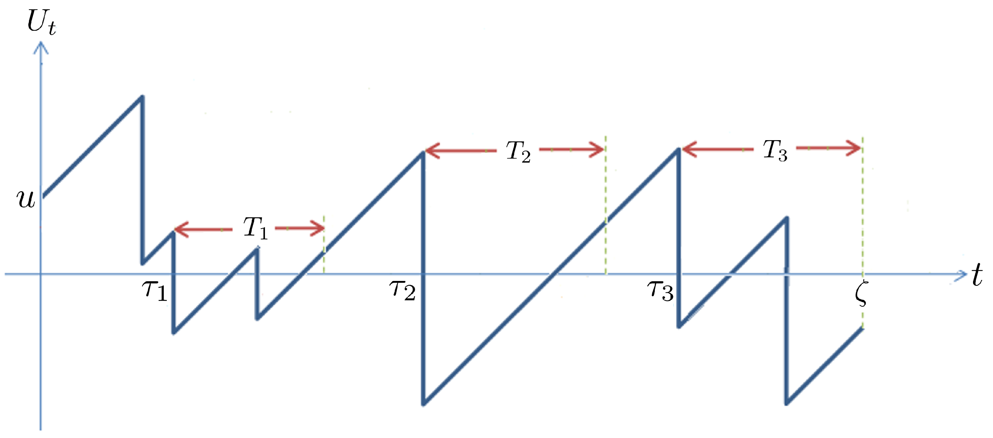
2.1. Modified Parisian Ruin Time and Gerber–Shiu Function

With Erlangization in mind, we let ${\left\{T_k\right\}}_{k=1}^{\infty }$ be an i.i.d. sequence of Erlang(n) random variables with common density

$$f_T\left(t\right)=\frac{{\gamma }^n{t}^{n-1}{e}^{-\gamma t}}{(n-1)!},t>0,$$

where $\gamma >0$ is the rate parameter. Here, $T_k$ refers to the k-th grace period accompanied by the k-th regulatory check. We construct a sequence of stopping times ${\left\{{\tau }_k\right\}}_{k=1}^{\infty }$ via

$${\tau }_k=\left\{\begin{array}{cc}inf\{t\ge 0:U(t)<0\},\hfill & k=1.\hfill \\ inf\{t\ge {\tau }_{k-1}+T_{k-1}:U\left(t\right)<0\},\hfill & k=2,3,4,\dots .\hfill \end{array}\right.$$

Clearly, ${\tau }_k$ marks the starting time of the k-th grace period, and in particular ${\tau }_1={\tau }_{\mathrm{CL}}$ is the classical ruin time. We further define $k^{*}=inf\{k\ge 1:U({\tau }_k+T_k)<0\}$, which keeps track of the first regulatory check where a negative surplus is observed at the end of the corresponding grace period. The modified Parisian ruin time is therefore $\zeta ={\tau }_{k^{*}}+T_{k^{*}}$. Figure 1 illustrates the random times defined above in relation to the modified Parisian ruin time for a particular sample path.

Recall that, under the classical ruin time ${\tau }_{\mathrm{CL}}$, the Gerber–Shiu expected discounted penalty function (Gerber and Shiu 1998) where the penalty only depends on the deficit is defined by

$${\varphi }_{\delta ,\mathrm{CL}}\left(u\right)={\mathbb{E}}_u[e^{-\delta {\tau }_{\mathrm{CL}}}w\left(\right|U\left({\tau }_{\mathrm{CL}}\right)\left|\right)1_{\{{\tau }_{\mathrm{CL}}<\infty \}}],u\ge 0.$$

(1)

Here, $\delta \ge 0$ can be regarded as the force of interest or the Laplace transform argument for ${\tau }_{\mathrm{CL}}$, and $w(·)$ is the “penalty function”. It is also known that ${\varphi }_{\delta ,\mathrm{CL}}\left(u\right)$ admits the representation

$${\varphi }_{\delta ,\mathrm{CL}}\left(u\right)={\int }_0^{\infty }w\left(y\right)h_{\delta ,\mathrm{CL}}\left(y\right|u)\mathrm{d}y,u\ge 0,$$

(2)

where the general formula for the discounted density $h_{\delta ,\mathrm{CL}}\left(y\right|u)$ of $\left|U\right({\tau }_{\mathrm{CL}}\left)\right|$ can be obtained by integrating out the first argument in Equation (2.40) of Gerber and Shiu (1998) concerning the discounted joint density of the surplus prior to ruin and the deficit at ruin.

To analyze the modified Parisian ruin time, we shall study the Gerber–Shiu function for which the penalty only depends on the deficit observed at such ruin time, namely

$${\varphi }_{\delta }\left(u\right)={\mathbb{E}}_u[e^{-\delta \zeta }w\left(\right|U\left(\zeta \right)\left|\right)1_{\{\zeta <\infty \}}],u\ge 0.$$

(3)

The discounted density of the associated deficit $\left|U\right(\zeta \left)\right|$ is defined by $h_{\delta }\left(y\right|u)$, which satisfies

$${\varphi }_{\delta }\left(u\right)={\int }_0^{\infty }w\left(y\right)h_{\delta }\left(y\right|u)\mathrm{d}y,u\ge 0.$$

(4)

If $\delta =0$ and $w(·)\equiv 1$, then ${\varphi }_{\delta }\left(u\right)$ reduces to the modified Parisian ruin probability $\psi \left(u\right)={\mathbb{P}}_u\{\zeta <\infty \}$.

2.2. Discounted Density of the Increment in a Grace Period

Note that when the surplus process downcrosses level zero at time ${\tau }_k$ (where $k=1,2,\dots$), a shortfall of magnitude $\left|U\right({\tau }_k\left)\right|$ is recorded. In order to tell whether ruin or recovery occurs at time ${\tau }_k+T_k$, we need to know the difference between the surplus levels at time ${\tau }_k$ and at time ${\tau }_k+T_k$. By virtue of spatial homogeneity, the change $U\left({\tau }_k\right)-U({\tau }_k+T_k)$ has the same distribution as ${\sum }_{i=1}^{N\left(T\right)}{Y}_i-cT$ (where T is a generic random variable with density $f_T(·)$). Due to the discount factor embedded in the Gerber–Shiu function, we have to keep track of the time T as well. From Section 3.2 of Albrecher et al. (2013), the joint Laplace transform of $(T,{\sum }_{i=1}^{N\left(T\right)}{Y}_i-cT)$ can be represented as

$$\mathbb{E}\left[e^{-\delta T-s({\sum }_{i=1}^{N\left(T\right)}{Y}_i-cT)}\right]={\int }_{-\infty }^{\infty }{e}^{-sy}{g}_{\delta }\left(y\right)\mathrm{d}y,$$

(5)

where $g_{\delta }\left(y\right)$ (for $-\infty <y<\infty$) is the discounted density of the increment ${\sum }_{i=1}^{N\left(T\right)}{Y}_i-cT$. It is convenient to decompose $g_{\delta }\left(y\right)$ as

$$g_{\delta }\left(y\right)=g_{\delta ,-}(-y)1_{\{y<0\}}+g_{\delta ,+}\left(y\right)1_{\{y>0\}}$$

(6)

so that $g_{\delta ,-}(·)$ (resp. $g_{\delta ,+}(·)$) represents the case where ${\sum }_{i=1}^{N\left(T\right)}{Y}_i-cT$ is negative (resp. positive) and there is a net gain (resp. net loss) during a grace period. While general expressions for $g_{\delta ,-}(·)$ and $g_{\delta ,+}(·)$ are available in Albrecher et al. (2013, Section 3.2), the key to the derivation of the Gerber–Shiu function in Section 3.1 relies on the “Erlang” form of the density $g_{\delta ,-}\left(y\right)$ in Equation (3.15), therein given by

$$g_{\delta ,-}\left(y\right)=\sum _{j=1}^n{A}_j\frac{y^{j-1}{e}^{-{\rho }_{\gamma +\delta }y}}{(j-1)!},y>0,$$

(7)

where $A_j$s are constants that do not depend on y, and ${\rho }_{\gamma +\delta }$ is a Lundberg root. Specifically, for $x\ge 0$, we define ${\rho }_x$ to be the unique non-negative root of the Lundberg-type equation

$$cs-(\lambda +x)+\lambda {\tilde{f}}_Y\left(s\right)=0.$$

(8)

Since $\gamma >0$ (and hence $\gamma +\delta >0$), it is known that ${\rho }_{\gamma +\delta }>0$. We shall delay the discussions about what $A_j$s and $g_{\delta ,+}(·)$ exactly are to the detailed example in Section 3.2 when claims are distributed as a combination of exponentials.

3. Main Results

3.1. General Expressions for Gerber–Shiu Function and Discounted Density of Deficit

We begin with the following theorem, which gives a general expression concerning the Gerber–Shiu function under our modified Parisian ruin time.

Theorem 1.

For a given choice of penalty function $w(·)$, the Gerber–Shiu function ${\varphi }_{\delta }\left(u\right)$ defined in (3) admits the representation

$${\varphi }_{\delta }\left(u\right)={\chi }_{\delta }\left(u\right)+\sum _{j=1}^n\left(\sum _{k=1}^{n-j+1}{A}_{j+k-1}{\phi }_{\delta ,k}\left(u\right)\right){\eta }_{\delta ,j}u\ge 0.$$

(9)

The intermediate quantities appearing above can be specified as follows. First, ${\chi }_{\delta }\left(u\right)$ is given by

$${\chi }_{\delta }\left(u\right)={\int }_0^{\infty }w\left(z\right){\xi }_{\delta }\left(z\right|u)\mathrm{d}z,u\ge 0,$$

(10)

where the function

$${\xi }_{\delta }\left(z\right|u)={\int }_0^z{g}_{\delta ,+}(z-y)h_{\delta ,\mathrm{CL}}\left(y\right|u)\mathrm{d}y+{\int }_z^{\infty }{g}_{\delta ,-}(y-z)h_{\delta ,\mathrm{CL}}\left(y\right|u)\mathrm{d}y,u,z\ge 0,$$

(11)

is expressed in terms of (i) the discounted densities $g_{\delta ,-}(·)$ and $g_{\delta ,+}(·)$ of the increment defined in Section 2.2; and (ii) the discounted density $h_{\delta ,\mathrm{CL}}(·|u)$ of the classical deficit $\left|U\right({\tau }_{\mathrm{CL}}\left)\right|$ defined via (2). Second, ${\left\{A_i\right\}}_{i=1}^n$ are constants associated with the representation (7) of $g_{\delta ,-}(·)$. Third, the quantity

$${\phi }_{\delta ,k}\left(u\right)={\int }_0^{\infty }\frac{y^{k-1}{e}^{-{\rho }_{\gamma +\delta }y}}{(k-1)!}{h}_{\delta ,\mathrm{CL}}\left(y\right|u)\mathrm{d}y,u\ge 0;k=1,2,\dots ,n,$$

(12)

is the classical Gerber–Shiu function ${\varphi }_{\delta ,\mathrm{CL}}\left(u\right)$ in (1) evaluated under the penalty function $w\left(y\right)=y^{k-1}{e}^{-{\rho }_{\gamma +\delta }y}/(k-1)!$, where ${\rho }_{\gamma +\delta }$ is the unique positive root of (8) at $x=\gamma +\delta$. Fourth, the constants ${\left\{{\eta }_{\delta ,j}\right\}}_{j=1}^n$ can be solved from the system of n linear equations

$${\eta }_{\delta ,i}={\int }_0^{\infty }\frac{u^{i-1}{e}^{-{\rho }_{\gamma +\delta }u}}{(i-1)!}{\chi }_{\delta }\left(u\right)\mathrm{d}u+\sum _{j=1}^n\left(\sum _{k=1}^{n-j+1}{A}_{j+k-1}{\int }_0^{\infty }\frac{u^{i-1}{e}^{-{\rho }_{\gamma +\delta }u}}{(i-1)!}{\phi }_{\delta ,k}\left(u\right)\mathrm{d}u\right){\eta }_{\delta ,j},i=1,2,\dots ,n.$$

(13)

Proof. 

Modified Parisian ruin cannot occur if the surplus process does not fall below zero. Therefore, we first condition the deficit $\left|U\right({\tau }_{\mathrm{CL}}\left)\right|$ at the classical ruin time ${\tau }_{\mathrm{CL}}$ to be equal to $y>0$. There are three cases depending on the increment of the surplus process during the grace period from time ${\tau }_{\mathrm{CL}}$ to time ${\tau }_{\mathrm{CL}}+T_1$:

• if there is a positive net loss of $z>0$ (with discounted density $g_{\delta ,+}(·)$), then ruin happens with a deficit of $\left|U\right(\zeta \left)\right|=y+z$;
• if there is a positive net gain of $z\in (0,y)$ (with discounted density $g_{\delta ,-}(·)$), then the gain is insufficient for the process to recover to a non-negative surplus and ruin happens with a deficit of $\left|U\right(\zeta \left)\right|=y-z$; and
• if there is a positive net gain of $z\ge y$, then the process recovers and restarts at the newly achieved non-negative surplus level $z-y$.

With the above arguments, we arrive at the integral equation

$${\varphi }_{\delta }\left(u\right)={\int }_0^{\infty }\left({\int }_0^{\infty }w(y+z)g_{\delta ,+}\left(z\right)\mathrm{d}z+{\int }_0^{y}w(y-z)g_{\delta ,-}\left(z\right)\mathrm{d}z+{\int }_y^{\infty }{\varphi }_{\delta }(z-y)g_{\delta ,-}\left(z\right)\mathrm{d}z\right)h_{\delta ,\mathrm{CL}}\left(y\right|u)\mathrm{d}y.$$

(14)

To simplify the above equation, it is first noted that the sum of the first two double integrals can be expressed as

$$\begin{array}{cc}\hfill & {\int }_0^{\infty }\left({\int }_0^{\infty }w(y+z)g_{\delta ,+}\left(z\right)\mathrm{d}z+{\int }_0^{y}w(y-z)g_{\delta ,-}\left(z\right)\mathrm{d}z\right)h_{\delta ,\mathrm{CL}}\left(y\right|u)\mathrm{d}y\hfill \\ \hfill =& {\int }_0^{\infty }\left({\int }_y^{\infty }w\left(z\right)g_{\delta ,+}(z-y)\mathrm{d}z\right)h_{\delta ,\mathrm{CL}}\left(y\right|u)\mathrm{d}y+{\int }_0^{\infty }\left({\int }_0^{y}w\left(z\right)g_{\delta ,-}(y-z)\mathrm{d}z\right)h_{\delta ,\mathrm{CL}}\left(y\right|u)\mathrm{d}y\hfill \\ \hfill =& {\int }_0^{\infty }w\left(z\right)\left({\int }_0^z{g}_{\delta ,+}(z-y)h_{\delta ,\mathrm{CL}}\left(y\right|u)\mathrm{d}y+{\int }_z^{\infty }{g}_{\delta ,-}(y-z)h_{\delta ,\mathrm{CL}}\left(y\right|u)\mathrm{d}y\right)\mathrm{d}z\hfill \\ \hfill =& {\chi }_{\delta }\left(u\right),\hfill \end{array}$$

(15)

where the definitions (10) and (11) have been used in the last equality. Meanwhile, with the help of (7), the third integral inside the big bracket of (14) is found to be

$$\begin{array}{cc}\hfill {\int }_y^{\infty }{\varphi }_{\delta }(z-y)g_{\delta ,-}\left(z\right)\mathrm{d}z=& \sum _{j=1}^n\frac{A_j}{(j-1)!}{\int }_0^{\infty }{\varphi }_{\delta }\left(z\right){(y+z)}^{j-1}{e}^{-{\rho }_{\gamma +\delta }(y+z)}\mathrm{d}z\hfill \\ \hfill =& \sum _{j=1}^n\frac{A_j}{(j-1)!}\sum _{k=1}^j\left(\genfrac{}{}{0pt}{}{j-1}{k-1}\right)\left({\int }_0^{\infty }{z}^{j-k}{e}^{-{\rho }_{\gamma +\delta }z}{\varphi }_{\delta }\left(z\right)\mathrm{d}z\right)y^{k-1}{e}^{-{\rho }_{\gamma +\delta }y}\hfill \\ \hfill =& \sum _{k=1}^n\frac{y^{k-1}{e}^{-{\rho }_{\gamma +\delta }y}}{(k-1)!}\sum _{j=k}^n{A}_j{\int }_0^{\infty }\frac{z^{j-k}{e}^{-{\rho }_{\gamma +\delta }z}}{(j-k)!}{\varphi }_{\delta }\left(z\right)\mathrm{d}z\hfill \\ \hfill =& \sum _{k=1}^n\frac{y^{k-1}{e}^{-{\rho }_{\gamma +\delta }y}}{(k-1)!}\sum _{j=1}^{n-k+1}{A}_{j+k-1}{\int }_0^{\infty }\frac{z^{j-1}{e}^{-{\rho }_{\gamma +\delta }z}}{(j-1)!}{\varphi }_{\delta }\left(z\right)\mathrm{d}z\hfill \\ \hfill =& \sum _{j=1}^n{\eta }_{\delta ,j}\sum _{k=1}^{n-j+1}{A}_{j+k-1}\frac{y^{k-1}{e}^{-{\rho }_{\gamma +\delta }y}}{(k-1)!},\hfill \end{array}$$

where

$${\eta }_{\delta ,j}={\int }_0^{\infty }\frac{z^{j-1}{e}^{-{\rho }_{\gamma +\delta }z}}{(j-1)!}{\varphi }_{\delta }\left(z\right)\mathrm{d}z,j=1,2,\dots ,n.$$

(16)

Utilizing the definition (12), the last double integral in (14) becomes

$${\int }_0^{\infty }\left({\int }_y^{\infty }{\varphi }_{\delta }(z-y)g_{\delta ,-}\left(z\right)\mathrm{d}z\right)h_{\delta ,\mathrm{CL}}\left(y\right|u)\mathrm{d}y=\sum _{j=1}^n{\eta }_{\delta ,j}\sum _{k=1}^{n-j+1}{A}_{j+k-1}{\phi }_{\delta ,k}\left(u\right).$$

This, together with (15), confirms that the representation (9) is valid.

Note that each ${\eta }_{\delta ,j}$ in (16) is expressed in terms of the Gerber–Shiu function ${\varphi }_{\delta }(·)$ itself and has not been completely determined. It remains to show that ${\left\{{\eta }_{\delta ,j}\right\}}_{j=1}^n$ satisfies the linear equations specified in (13). This is seen to be true by multiplying both sides of (9) by $u^{i-1}{e}^{-{\rho }_{\gamma +\delta }u}/(i-1)!$ (for each $i=1,2,\dots ,n$) and then integrating with respect to u from 0 to ∞. □

The system of linear equations in (13) can indeed be rewritten in a more compact manner. To this end, we start by defining the function

$${\Delta }_{\delta ,i}\left(z\right)={\int }_0^{\infty }\frac{u^{i-1}{e}^{-{\rho }_{\gamma +\delta }u}}{(i-1)!}{\xi }_{\delta }\left(z\right|u)\mathrm{d}u,z\ge 0;i=1,2,\dots ,n.$$

The first integral on the right-hand side of (13) can now be equivalently expressed as

$${\int }_0^{\infty }\frac{u^{i-1}{e}^{-{\rho }_{\gamma +\delta }u}}{(i-1)!}{\chi }_{\delta }\left(u\right)\mathrm{d}u={\int }_0^{\infty }w\left(z\right){\Delta }_{\delta ,i}\left(z\right)\mathrm{d}z.$$

(17)

We further define the n-dimensional column vectors ${\mathit{\eta }}_{\delta }$ and ${\mathbf{\Delta }}_{\delta }\left(z\right)$ with i-th elements ${\eta }_{\delta ,i}$ and ${\Delta }_{\delta ,i}\left(z\right)$, respectively, as well as the n-dimensional square matrix ${\mathbf{\Gamma }}_{\delta }$ with the $(i,j)$-th element

$${\left[{\mathbf{\Gamma }}_{\delta }\right]}_{ij}=\sum _{k=1}^{n-j+1}{A}_{j+k-1}{\int }_0^{\infty }\frac{u^{i-1}{e}^{-{\rho }_{\gamma +\delta }u}}{(i-1)!}{\phi }_{\delta ,k}\left(u\right)\mathrm{d}u.$$

(18)

Then, (13) becomes

$${\mathit{\eta }}_{\delta }={\int }_0^{\infty }w\left(z\right){\mathbf{\Delta }}_{\delta }\left(z\right)\mathrm{d}z+{\mathbf{\Gamma }}_{\delta }{\mathit{\eta }}_{\delta },$$

with solution

$${\mathit{\eta }}_{\delta }={(\mathbf{I}-{\mathbf{\Gamma }}_{\delta })}^{-1}{\int }_0^{\infty }w\left(z\right){\mathbf{\Delta }}_{\delta }\left(z\right)\mathrm{d}z,$$

(19)

where $\mathbf{I}$ is an identity matrix of dimension n, and the invertibility of the matrix $\mathbf{I}-{\mathbf{\Gamma }}_{\delta }$ is assumed.

The above vectors/matrices are also useful for us to obtain a compact expression for the discounted density of deficit $\left|U\right(\zeta \left)\right|$ in the following corollary.

Corollary 1.

The discounted density $h_{\delta }\left(y\right|u)$ of the deficit $\left|U\right(\zeta \left)\right|$ defined via (4) admits the representation

$$h_{\delta }\left(y\right|u)={\xi }_{\delta }\left(y\right|u)+{\mathit{\sigma }}_{\delta }\left(u\right){(\mathbf{I}-{\mathbf{\Gamma }}_{\delta })}^{-1}{\mathbf{\Delta }}_{\delta }\left(y\right),u,y\ge 0,$$

(20)

where ${\mathit{\sigma }}_{\delta }\left(u\right)$ is an n-dimensional row vector with j-element ${\sum }_{k=1}^{n-j+1}{A}_{j+k-1}{\phi }_{\delta ,k}\left(u\right)$.

Proof. 

By applying the definition of ${\mathit{\sigma }}_{\delta }\left(u\right)$ as well as (10) and (19) to (9), we can express ${\varphi }_{\delta }\left(u\right)$ as

$${\varphi }_{\delta }\left(u\right)={\int }_0^{\infty }w\left(z\right){\xi }_{\delta }\left(z\right|u)\mathrm{d}z+{\mathit{\sigma }}_{\delta }\left(u\right){(\mathbf{I}-{\mathbf{\Gamma }}_{\delta })}^{-1}{\int }_0^{\infty }w\left(z\right){\mathbf{\Delta }}_{\delta }\left(z\right)\mathrm{d}z.$$

Comparison with (4) yields the desired result (20). □

3.2. Laplace Transform of Ruin Time When Claims Follow a Combination of Exponentials

In this subsection, it is assumed that the claim amounts are distributed as a combination of exponentials with density

$$f_Y\left(y\right)=\sum _{j=1}^m{q}_j{\alpha }_j{e}^{-{\alpha }_{j}y},y>0,$$

where ${\alpha }_j$s are positive and distinct while $q_j$s are non-zero numbers that sum to one. The class of combinations of exponentials is known to be dense in the set of positive continuous distributions, and it has become a popular choice for the claim amount distributions in insurance risk processes. Interested readers are referred to Dufresne (2007) for fitting algorithms of this class of distributions.

With the above distributional assumption, explicit formulas for the discounted densities $g_{\delta ,-}\left(y\right)$, $g_{\delta ,+}\left(y\right)$ and $h_{\delta ,\mathrm{CL}}\left(y\right|u)$ are available as follows. First, the Laplace transform of the claim amounts can be written as ${\tilde{f}}_Y\left(s\right)=Q_2\left(s\right)/Q_1\left(s\right)$, where

$$Q_1\left(s\right)=\prod _{i=1}^m({\alpha }_i+s)\mathrm{and}{Q}_2\left(s\right)=\sum _{j=1}^m{q}_j{\alpha }_j\prod _{i=1,i\ne j}^m({\alpha }_i+s).$$

In this case, the Lundberg-type Equation (8) at $x=\gamma +\delta$ has m roots with negative real parts. Denoting these roots by ${\{-R_{\gamma +\delta ,i}\}}_{i=1}^m$, it is known from Albrecher et al. (2013, Section 4) that

$$g_{\delta ,+}\left(y\right)=\sum _{i=1}^m\sum _{j=1}^n{B}_{ij}\frac{y^{j-1}{e}^{-R_{\gamma +\delta ,i}y}}{(j-1)!},y>0,$$

(21)

and the coefficients $A_j$s in (7) and $B_{ij}$s above are obtained from the partial fractions expansion

$${\left(\frac{\gamma }{c}\right)}^n\frac{{\left[Q_1\left(s\right)\right]}^n}{{({\rho }_{\gamma +\delta }-s)}^n{\prod }_{i=1}^m{(s+R_{\gamma +\delta ,i})}^n}=\sum _{j=1}^n\frac{A_j}{{({\rho }_{\gamma +\delta }-s)}^j}+\sum _{i=1}^m\sum _{j=1}^n\frac{B_{ij}}{{(s+R_{\gamma +\delta ,i})}^j}.$$

(22)

Concerning $h_{\delta ,\mathrm{CL}}\left(y\right|u)$, from Gerber and Shiu (2005, Equations (7.8) and (7.9)), we have

$$h_{\delta ,\mathrm{CL}}\left(y\right|u)=\sum _{j=1}^m\sum _{k=1}^m{C}_{jk}{e}^{-R_{\delta ,k}u-{\alpha }_{j}y},u,y\ge 0,$$

(23)

where

$$C_{jk}=\left(\prod _{\ell =1,\ell \ne j}^m\frac{-R_{\delta ,k}+{\alpha }_{\ell }}{{\alpha }_j-{\alpha }_{\ell }}\right)\left(\prod _{i=1,i\ne k}^m\frac{{\alpha }_j-R_{\delta ,i}}{-R_{\delta ,k}+R_{\delta ,i}}\right)({\alpha }_j-R_{\delta ,k}),j,k=1,2,\dots ,m.$$

(24)

Next, we shall evaluate the necessary intermediate quantities in relation to the general results in Theorem 1. Using (23), we readily see that (12) is found to be

$${\phi }_{\delta ,k}\left(u\right)=\sum _{i=1}^m\sum _{j=1}^m\frac{C_{ij}}{{({\rho }_{\gamma +\delta }+{\alpha }_i)}^k}{e}^{-R_{\delta ,j}u}.$$

(25)

Therefore, (18) is given by

$${\left[{\mathbf{\Gamma }}_{\delta }\right]}_{ij}=\sum _{k=1}^{n-j+1}{A}_{j+k-1}\sum _{\ell =1}^m\sum _{a=1}^m\frac{C_{\ell a}}{{({\rho }_{\gamma +\delta }+{\alpha }_{\ell })}^k}\frac{1}{{({\rho }_{\gamma +\delta }+R_{\delta ,a})}^i}.$$

(26)

Moreover, substituting (7), (21) and (23) into (11) followed by a change of variables of integration yields

$$\begin{array}{cc}\hfill {\xi }_{\delta }\left(z\right|u)=& \sum _{i=1}^m\sum _{j=1}^n\sum _{\ell =1}^m\sum _{k=1}^m{B}_{ij}{C}_{\ell k}{\int }_0^z\frac{y^{j-1}{e}^{-R_{\gamma +\delta ,i}y}}{(j-1)!}{e}^{-R_{\delta ,k}u-{\alpha }_{\ell }(z-y)}\mathrm{d}y\hfill \\ \hfill & +\sum _{j=1}^n\sum _{\ell =1}^m\sum _{k=1}^m{A}_j{C}_{\ell k}{\int }_0^{\infty }\frac{y^{j-1}{e}^{-{\rho }_{\gamma +\delta }y}}{(j-1)!}{e}^{-R_{\delta ,k}u-{\alpha }_{\ell }(z+y)}\mathrm{d}y.\hfill \end{array}$$

(27)

Note that the function ${\chi }_{\delta }(·)$ defined in (10) depends on the choice of the penalty function. In what follows, it is further assumed that $w(·)\equiv 1$ so that ${\varphi }_{\delta }\left(u\right)$ becomes the Laplace transform of the modified Parisian ruin time. Consequently, ${\chi }_{\delta }(·)$ is simply the integral of (27) with respect to z. By changing the order of integration in the first term, we obtain

$$\begin{array}{cc}\hfill {\chi }_{\delta }\left(u\right)=& \sum _{i=1}^m\sum _{j=1}^n\sum _{\ell =1}^m\sum _{k=1}^m{B}_{ij}{C}_{\ell k}\left[{\int }_0^{\infty }\left({\int }_y^{\infty }{e}^{-{\alpha }_{\ell }(z-y)}\mathrm{d}z\right)\frac{y^{j-1}{e}^{-R_{\gamma +\delta ,i}y}}{(j-1)!}\mathrm{d}y\right]e^{-R_{\delta ,k}u}\hfill \\ \hfill & +\sum _{j=1}^n\sum _{\ell =1}^m\sum _{k=1}^m{A}_j{C}_{\ell k}\left({\int }_0^{\infty }\frac{y^{j-1}{e}^{-({\rho }_{\gamma +\delta }+{\alpha }_{\ell })y}}{(j-1)!}\mathrm{d}y\right)\left({\int }_0^{\infty }{e}^{-{\alpha }_{\ell }z}\mathrm{d}z\right)e^{-R_{\delta ,k}u}\hfill \\ \hfill =& \sum _{\ell =1}^m\sum _{k=1}^m\frac{C_{\ell k}}{{\alpha }_{\ell }}\left(\sum _{j=1}^n\frac{A_j}{{({\rho }_{\gamma +\delta }+{\alpha }_{\ell })}^j}+\sum _{i=1}^m\sum _{j=1}^n\frac{B_{ij}}{R_{\gamma +\delta ,i}^j}\right)e^{-R_{\delta ,k}u}.\hfill \end{array}$$

(28)

Then, using the identity (17) and the above result, the i-th element of ${\int }_0^{\infty }{\mathbf{\Delta }}_{\delta }\left(z\right)\mathrm{d}z$ is

$${\int }_0^{\infty }{\Delta }_{\delta ,i}\left(z\right)\mathrm{d}z=\sum _{\ell =1}^m\sum _{k=1}^m\frac{C_{\ell k}}{{\alpha }_{\ell }}\left(\sum _{j=1}^n\frac{A_j}{{({\rho }_{\gamma +\delta }+{\alpha }_{\ell })}^j}+\sum _{a=1}^m\sum _{j=1}^n\frac{B_{aj}}{R_{\gamma +\delta ,a}^j}\right)\frac{1}{{({\rho }_{\gamma +\delta }+R_{\delta ,k})}^i}.$$

(29)

We now have all the necessary pieces to compute the Laplace transform of the modified Parisian ruin time, and the procedure is summarized as follows.

• Step 1: Find the roots of the Lundberg Equation (8) at $x=\gamma +\delta$. Denote the positive root by ${\rho }_{\gamma +\delta }$ and the m roots with negative real parts by ${\{-R_{\gamma +\delta ,j}\}}_{j=1}^m$. Additionally, find the m roots with negative real parts of the Lundberg Equation (8) at $x=\delta$ and denote them by ${\{-R_{\delta ,j}\}}_{j=1}^m$.
• Step 2: Determine the coefficients $A_j$s and $B_{ij}$s from the partial fractions expansion (22).
• Step 3: Compute $C_{jk}$s using (24).
• Step 4: Compute ${\mathit{\eta }}_{\delta }$ using (19) (at $w(·)\equiv 1$), where the $(i,j)$-th element of ${\mathbf{\Gamma }}_{\delta }$ is given by (26) and the i-th element of ${\int }_0^{\infty }{\mathbf{\Delta }}_{\delta }\left(z\right)\mathrm{d}z$ is given by (29).
• Step 5: Compute ${\varphi }_{\delta }\left(u\right)$ with (9), where ${\chi }_{\delta }\left(u\right)$ and ${\phi }_{\delta ,k}\left(u\right)$ are given by (28) and (25), respectively, and ${\left\{{\eta }_{\delta ,j}\right\}}_{j=1}^n$ are the elements of ${\eta }_{\delta }$ from Step 4.

4. Numerical Illustrations

This section aims to provide numerical examples for the modified Parisian ruin probability using the results from Section 3.2. In order to compare with the standard Parisian ruin probability in Landriault et al. (2014, Section 4), who looked at the case of exponential claims with Erlang grace periods, we shall closely follow the parameters therein. It is always assumed that the claims arrive at rate $\lambda =1/3$ and the premium is collected at rate $c=4$. We first consider exponential claim amounts with mean 9 (so that $f_Y\left(y\right)=(1/9)e^{-(1/9)y}$) and calculate the modified Parisian ruin probability $\psi \left(u\right)={\mathbb{P}}_u\{\zeta <\infty \}$ (by letting $\delta =0$ in Section 3.2). In particular, we shall fix the mean of the Erlang grace periods to be $\mathbb{E}\left[T\right]=n/\gamma =1,2,5,10$ in turn while increasing n (and $\gamma$) to see the performance of Erlangization in approximating deterministic grace periods.

Table 1. Standard and modified Parisian ruin probabilities under exponential claims when $u=0$.

n	$\mathbb{E}\left[\mathit{T}\right]=1$		$\mathbb{E}\left[\mathit{T}\right]=2$		$\mathbb{E}\left[\mathit{T}\right]=5$		$\mathbb{E}\left[\mathit{T}\right]=10$
	Standard	Modified	Standard	Modified	Standard	Modified	Standard	Modified
1	0.6886	0.6886	0.6478	0.6478	0.5676	0.5676	0.4867	0.4867
5	0.6767	0.6786	0.6195	0.6275	0.5020	0.5322	0.3879	0.4423
10	0.6748	0.6770	0.6144	0.6241	0.4910	0.5273	0.3737	0.4370
15	0.6741	0.6764	0.6126	0.6229	0.4873	0.5257	0.3690	0.4353
20	0.6737	0.6761	0.6117	0.6223	0.4854	0.5250	0.3667	0.4344
25	0.6735	0.6759	0.6112	0.6219	0.4842	0.5245	0.3653	0.4339
30	0.6733	0.6758	0.6108	0.6217	0.4835	0.5242	0.3644	0.4336
35	0.6732	0.6757	0.6105	0.6215	0.4829	0.5240	0.3637	0.4333
40	0.6732	0.6756	0.6103	0.6214	0.4825	0.5238	0.3633	0.4331
45	0.6731	0.6755	0.6102	0.6213	0.4822	0.5237	0.3629	0.4330
50	0.6731	0.6755	0.6100	0.6212	0.4820	0.5236	0.3626	0.4329

and

Table 2. Standard and modified Parisian ruin probabilities under exponential claims when $u=50$.

n	$\mathbb{E}\left[\mathit{T}\right]=1$		$\mathbb{E}\left[\mathit{T}\right]=2$		$\mathbb{E}\left[\mathit{T}\right]=5$		$\mathbb{E}\left[\mathit{T}\right]=10$
	Standard	Modified	Standard	Modified	Standard	Modified	Standard	Modified
1	0.1717	0.1717	0.1615	0.1615	0.1415	0.1415	0.1213	0.1213
5	0.1687	0.1692	0.1545	0.1565	0.1252	0.1327	0.0967	0.1103
10	0.1683	0.1688	0.1532	0.1556	0.1224	0.1315	0.0932	0.1090
15	0.1681	0.1687	0.1528	0.1553	0.1215	0.1311	0.0920	0.1085
20	0.1680	0.1686	0.1525	0.1552	0.1210	0.1309	0.0914	0.1083
25	0.1679	0.1685	0.1524	0.1551	0.1207	0.1308	0.0911	0.1082
30	0.1679	0.1685	0.1523	0.1550	0.1206	0.1307	0.0909	0.1081
35	0.1679	0.1685	0.1522	0.1550	0.1204	0.1306	0.0907	0.1081
40	0.1679	0.1685	0.1522	0.1549	0.1203	0.1306	0.0906	0.1080
45	0.1679	0.1684	0.1521	0.1549	0.1202	0.1306	0.0905	0.1080
50	0.1678	0.1684	0.1521	0.1549	0.1202	0.1305	0.0904	0.1079

summarize the modified Parisian ruin probabilities for an initial surplus of $u=0$ and $u=50$, respectively, and the numerical values of the standard Parisian ruin probability from Landriault et al. (2014) are also reproduced here for easy comparison. For reference, the classical ruin probabilities are given by ${\mathbb{P}}_0\{{\tau }_{\mathrm{CL}}<\infty \}=0.7500$ and ${\mathbb{P}}_{50}\{{\tau }_{\mathrm{CL}}<\infty \}=0.1870$. The following observations are made from the tables along with some insights.

• When $n=1$, the two Parisian ruin probabilities are identical for each fixed pair of $(u,\mathbb{E}[T]$). This is a direct consequence of the memoryless property of exponential grace periods.
• The modified Parisian ruin probability ${\mathbb{P}}_u\{\zeta <\infty \}$ is smaller than the classical ruin probability ${\mathbb{P}}_u\{{\tau }_{\mathrm{CL}}<\infty \}$. This must be the case because modified Parisian ruin can only occur if the surplus process ever falls below zero. On the other hand, for fixed triplet $(u,\mathbb{E}[T],n)$, the modified Parisian ruin probability is no less than the standard Parisian ruin probability. Recall that, according to the definition of standard Parisian ruin, the business is deemed to have recovered as long as the surplus attains a non-negative level at any time point within the grace period. However, under the modified Parisian ruin, this is not sufficient to avoid ruin: the surplus has to be non-negative at the end of the grace period in order to survive the regulatory check. As a result, our proposed definition of ruin is more stringent than standard Parisian ruin from a regulatory point of view, and the modified Parisian ruin probability could potentially be a risk quantity to consider if one wishes to be conservative.
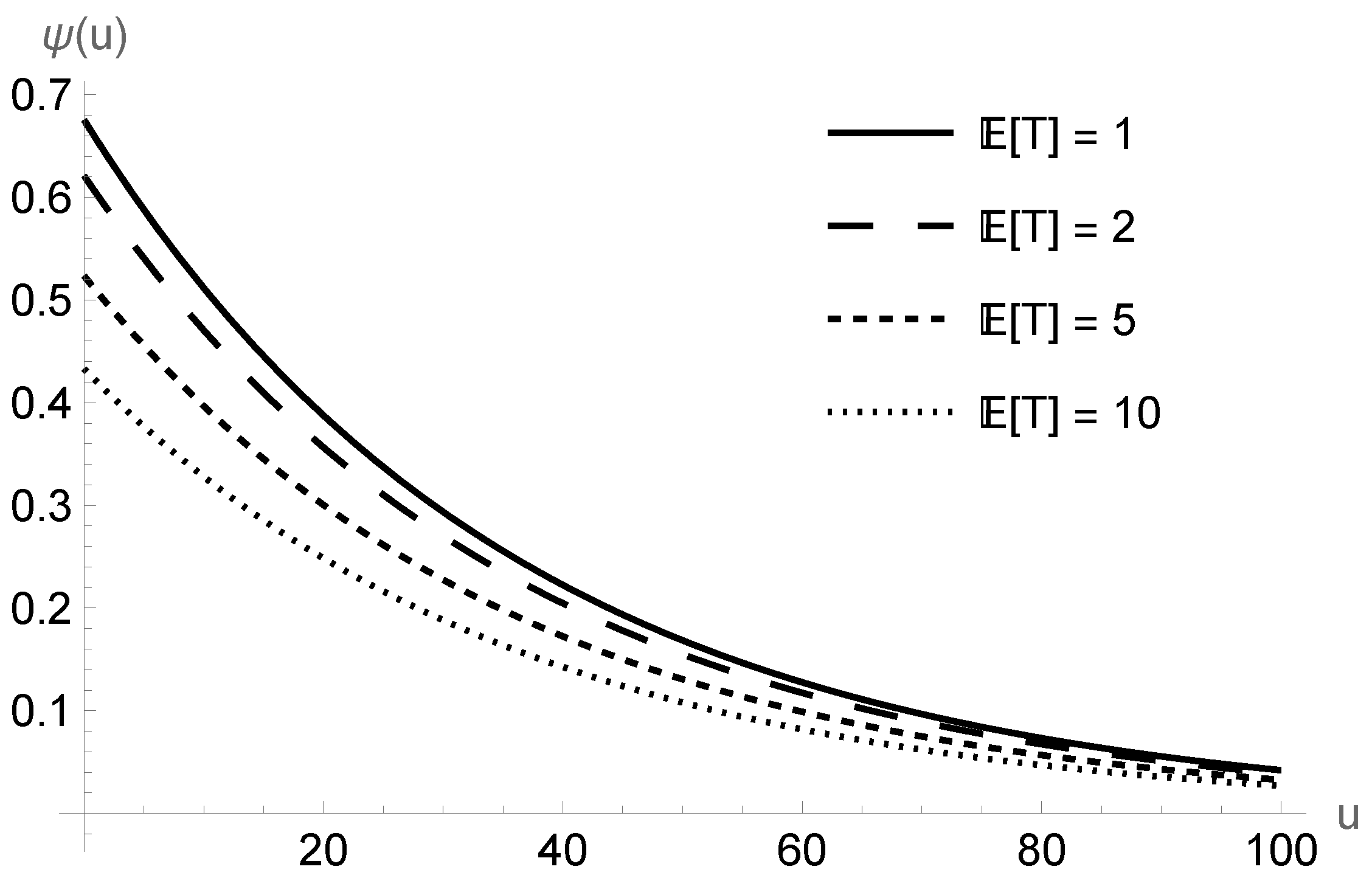
• For fixed $(n,u)$, the modified Parisian ruin probability $\psi \left(u\right)$ decreases when the expected grace period $\mathbb{E}\left[T\right]$ increases. For reference, in Figure 2, we have further plotted $\psi \left(u\right)$ as a function of u for $\mathbb{E}\left[T\right]=1,2,5,10$ in the case where $n=50$ to observe that the curves are ordered. Recall that the insurer’s surplus process has a positive trend under the positive loading condition. Therefore, the business is more likely to survive the regulatory check if it is given a longer grace period so that profits can be accumulated, thereby lowering the modified Parisian ruin probability.
• For fixed $(n,u)$, the difference between the two Parisian ruin probabilities increases in $\mathbb{E}\left[T\right]$. Intuitively, when $\mathbb{E}\left[T\right]$ is small, there is insufficient time for the insurer to collect a premium for recovery. Consequently, it is more likely for the surplus process to remain negative for the entire grace period, leading to ruin under both definitions and hence a small difference in the ruin probabilities.
• As n increases down each column, the modified Parisian ruin probability converges because one approaches the case of deterministic grace periods thanks to the Erlangization procedure. The use of moderate values of n (around $n=20$) often leads to excellent results.

Figure 2. Modified Parisian ruin probability $\psi \left(u\right)$ for $\mathbb{E}\left[T\right]=1,2,5,10$ using $n=50$.

Figure 2. Modified Parisian ruin probability $\psi \left(u\right)$ for $\mathbb{E}\left[T\right]=1,2,5,10$ using $n=50$.

Next, we are interested in the modified Parisian ruin probability when the claim amounts deviate from the exponential assumption. Specifically, the following two claim distributions will be considered:

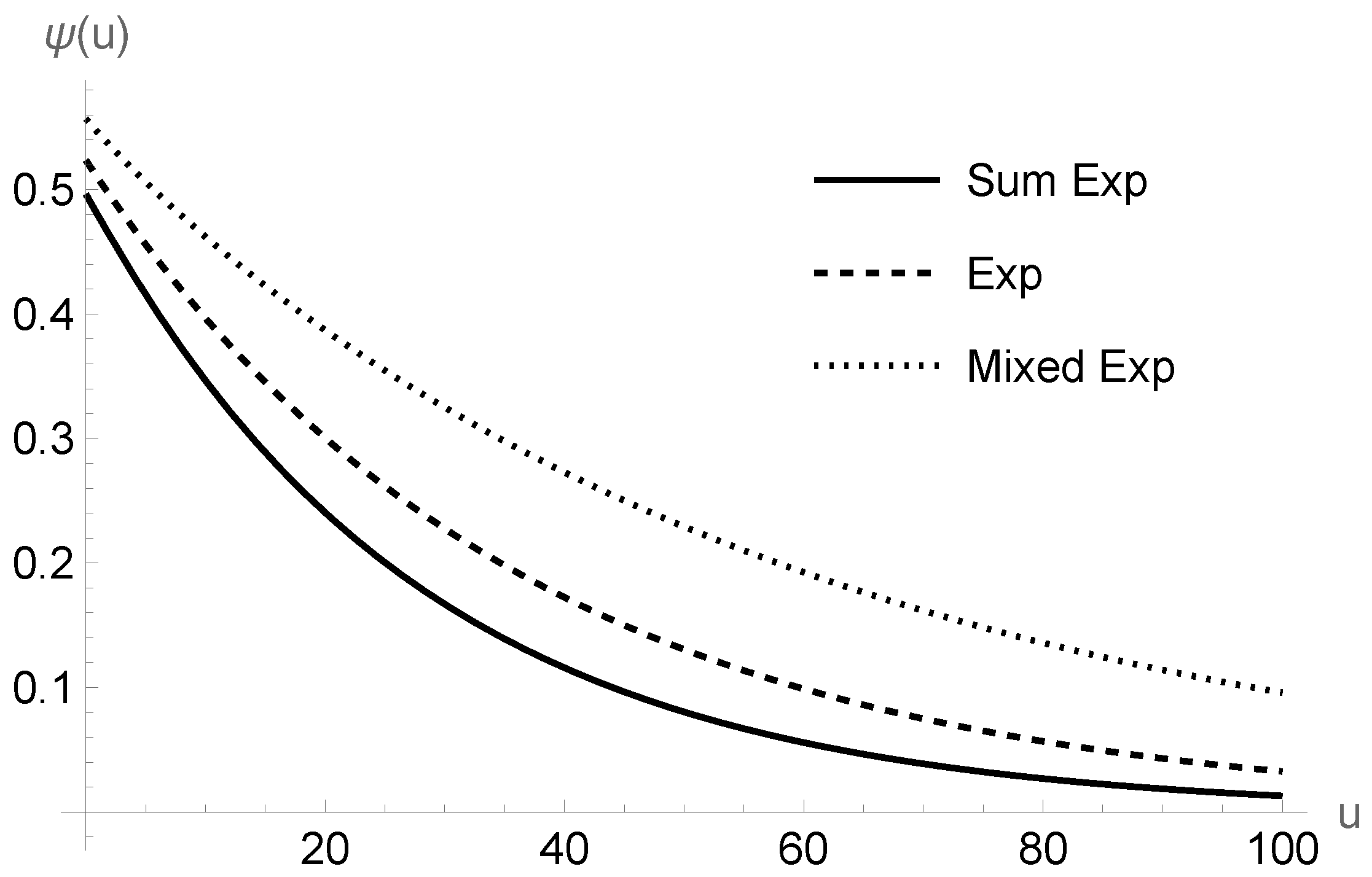
• A sum of two independent exponential variables (possessing respective means 3 and 6) with density $f_Y\left(y\right)=2(1/6)e^{-(1/6)y}-(1/3)e^{-(1/3)y}$;
• A mixture of two exponentials with density $f_Y\left(y\right)=(1/3)(1/18)e^{-(1/18)y}+(2/3)(2/9)$$e^{-(2/9)y}$.

Both distributions have the same mean of 9 while their variances are 45 and 162, respectively (compared to a variance of 81 in the exponential case). When $u=0$, the classical ruin probability is ${\mathbb{P}}_0\{{\tau }_{\mathrm{CL}}<\infty \}=0.7500$ for both claim distributions, whereas when $u=50$, the values of the probability ${\mathbb{P}}_{50}\{{\tau }_{\mathrm{CL}}<\infty \}$ are 0.1238 and 0.2933, respectively. The modified Parisian ruin probability values under these two claim distributions are provided in

Table 3. Modified Parisian ruin probabilities when claims are a sum of exponentials.

n	$\mathbb{E}\left[\mathit{T}\right]=1$		$\mathbb{E}\left[\mathit{T}\right]=2$		$\mathbb{E}\left[\mathit{T}\right]=5$		$\mathbb{E}\left[\mathit{T}\right]=10$
	$\mathit{u}=0$	$\mathit{u}=50$	$\mathit{u}=0$	$\mathit{u}=50$	$\mathit{u}=0$	$\mathit{u}=50$	$\mathit{u}=0$	$\mathit{u}=50$
1	0.6813	0.1110	0.6347	0.1031	0.5451	0.0883	0.4573	0.0740
5	0.6693	0.1086	0.6100	0.0988	0.5053	0.0818	0.4093	0.0663
10	0.6671	0.1082	0.6058	0.0980	0.5002	0.0810	0.4038	0.0654
15	0.6664	0.1081	0.6043	0.0978	0.4986	0.0807	0.4019	0.0651
20	0.6660	0.1080	0.6036	0.0977	0.4978	0.0806	0.4010	0.0649
25	0.6657	0.1080	0.6031	0.0976	0.4973	0.0805	0.4005	0.0649
30	0.6656	0.1079	0.6028	0.0975	0.4970	0.0805	0.4001	0.0648
35	0.6655	0.1079	0.6026	0.0975	0.4968	0.0804	0.3999	0.0648
40	0.6654	0.1079	0.6024	0.0975	0.4966	0.0804	0.3997	0.0647
45	0.6653	0.1079	0.6023	0.0975	0.4965	0.0804	0.3995	0.0647
50	0.6652	0.1079	0.6022	0.0974	0.4964	0.0804	0.3994	0.0647

and

Table 4. Modified Parisian ruin probabilities when claims are a mixture of exponentials.

n	$\mathbb{E}\left[\mathit{T}\right]=1$		$\mathbb{E}\left[\mathit{T}\right]=2$		$\mathbb{E}\left[\mathit{T}\right]=5$		$\mathbb{E}\left[\mathit{T}\right]=10$
	$\mathit{u}=0$	$\mathit{u}=50$	$\mathit{u}=0$	$\mathit{u}=50$	$\mathit{u}=0$	$\mathit{u}=50$	$\mathit{u}=0$	$\mathit{u}=50$
1	0.6943	0.2775	0.6600	0.2660	0.5930	0.2416	0.5237	0.2147
5	0.6853	0.2754	0.6433	0.2616	0.5641	0.2319	0.4857	0.2002
10	0.6838	0.2751	0.6406	0.2609	0.5600	0.2304	0.4809	0.1982
15	0.6833	0.2750	0.6397	0.2606	0.5587	0.2299	0.4793	0.1975
20	0.6830	0.2749	0.6393	0.2605	0.5580	0.2297	0.4785	0.1972
25	0.6829	0.2749	0.6390	0.2604	0.5576	0.2295	0.4780	0.1970
30	0.6827	0.2748	0.6388	0.2604	0.5573	0.2294	0.4777	0.1968
35	0.6827	0.2748	0.6387	0.2603	0.5571	0.2294	0.4775	0.1968
40	0.6826	0.2748	0.6386	0.2603	0.5570	0.2293	0.4773	0.1967
45	0.6826	0.2748	0.6385	0.2603	0.5569	0.2293	0.4772	0.1966
50	0.6825	0.2748	0.6384	0.2603	0.5568	0.2292	0.4771	0.1966

. Such probabilities exhibit a very similar pattern compared to the case of exponential claims, such as monotonicity in $\mathbb{E}\left[T\right]$ and convergence in the Erlangization procedure. More importantly, when we compare the modified Parisian ruin probabilities across the three claim amounts, it is clear that a claim distribution with a higher variance leads to a higher ruin probability. For easy comparison, we have also plotted in Figure 3 the modified Parisian ruin probability $\psi \left(u\right)$ under three claim distributions when $\mathbb{E}\left[T\right]=5$ and $n=50$, and the curves are ordered according to the claim variance. This intuitively makes sense because a higher claim variance will more likely lead to a larger shortfall when the surplus process falls below zero and hence it becomes more difficult for the process to recover when it is checked at the end of the grace period. Note that the case of mixed exponential claims leads to significantly higher ruin probability than the other two claim distributions when the initial surplus u is large, indicating that insurers need to be cautious with claims of high variance.

5. Concluding Remarks

In this paper, we have proposed a modification to the standard definition of Parisian ruin and derived an exact formula for the corresponding Gerber–Shiu function. Through numerical illustrations, it is demonstrated that our formulas can be easily computed, and we also suggest that the modified Parisian ruin probability is more conservative than the standard Parisian counterpart.

Extensions of our proposed model can potentially be considered in various directions. First, one may argue that, when the business is undergoing restructuring and reorganization during the grace period, the surplus process is allowed to follow different dynamics. In this case, we can replace $g_{\delta ,-}(·)$ and $g_{\delta ,+}(·)$ in (14) by $g_{\delta ,-}^{*}(·)$ and $g_{\delta ,+}^{*}(·)$, which are the discounted densities defined via (5) and (6), but with a possibly different premium rate, Poisson arrival rate and claim distribution. Second, a lower bankruptcy barrier $-b$ (for some $b>0$) may be incorporated such that ruin is declared immediately if the shortfall is larger than b when an excursion below zero begins at time ${\tau }_k$ for some $k=1,2,\dots$. Denoting the resulting Gerber–Shiu function by ${\varphi }_{\delta }(u;b)$, the integral Equation (14) is generalized to

$$\begin{array}{cc}\hfill {\varphi }_{\delta }(u;b)=& {\int }_0^b\left({\int }_0^{\infty }w(y+z)g_{\delta ,+}\left(z\right)\mathrm{d}z+{\int }_0^{y}w(y-z)g_{\delta ,-}\left(z\right)\mathrm{d}z+{\int }_y^{\infty }{\varphi }_{\delta }(z-y;b)g_{\delta ,-}\left(z\right)\mathrm{d}z\right)h_{\delta ,\mathrm{CL}}\left(y\right|u)\mathrm{d}y\hfill \\ \hfill & +{\int }_b^{\infty }w\left(y\right)h_{\delta ,\mathrm{CL}}\left(y\right|u)\mathrm{d}y,\hfill \end{array}$$

which can be solved in a similar manner to the proof of Theorem 1. Third, it will also be interesting to replace the compound Poisson model by a spectrally negative Lévy process. However, this extension is far from straightforward because we need to take into account the case where the process downcrosses zero by diffusion, and moreover the densities $g_{\delta ,-}(·)$ and $g_{\delta ,+}(·)$ are not known from the literature. We leave this as an open problem.

References

1. Albrecher, Hansjoerg, and Jevgenijs Ivanovs. 2013. A risk model with an observer in a Markov environment. Risks 1: 148–61. [Google Scholar] [CrossRef] [Green Version]
2. Albrecher, Hansjoerg, and Jevgenijs Ivanovs. 2017. Strikingly simple identities relating exit problems for Lévy processes under continuous and Poisson observations. Stochastic Processes and Their Applications 127: 643–56. [Google Scholar] [CrossRef] [Green Version]
3. Albrecher, Hansjoerg, and Volkmar Lautscham. 2013. From ruin to bankruptcy for compound Poisson surplus processes. ASTIN Bulletin 43: 213–43. [Google Scholar] [CrossRef] [Green Version]
4. Albrecher, Hansjoerg, Eric C. K. Cheung, and Stefan Thonhauser. 2011a. Randomized observation periods for the compound Poisson risk model: Dividends. ASTIN Bulletin 41: 645–72. [Google Scholar]
5. Albrecher, Hansjoerg, Eric C. K. Cheung, and Stefan Thonhauser. 2013. Randomized observation periods for the compound Poisson risk model: The discounted penalty function. Scandinavian Actuarial Journal 2013: 424–52. [Google Scholar] [CrossRef]
6. Albrecher, Hansjoerg, Hans U. Gerber, and Elias S. W. Shiu. 2011b. The optimal dividend barrier in the Gamma-Omega model. European Actuarial Journal 1: 43–55. [Google Scholar] [CrossRef] [Green Version]
7. Albrecher, Hansjoerg, Jevgenijs Ivanovs, and Xiaowen Zhou. 2016. Exit identities for Lévy processes observed at Poisson arrival times. Bernoulli 22: 1364–82. [Google Scholar] [CrossRef] [Green Version]
8. Antill, Samuel, and Steven R. Grenadier. 2019. Optimal capital structure and bankruptcy choice: Dynamic bargaining versus liquidation. Journal of Financial Economics 133: 198–224. [Google Scholar] [CrossRef]
9. Asmussen, Soren, Florin Avram, and Miguel Usabel. 2002. Erlangian approximations for finite-horizon ruin probabilities. ASTIN Bulletin 32: 267–81. [Google Scholar] [CrossRef] [Green Version]
10. Baurdoux, E. J., J. C. Pardo, J. L. Pérez, and J. F. Renaud. 2016. Gerber-Shiu distribution at Parisian ruin for Lévy insurance risk processes. Journal of Applied Probability 53: 572–84. [Google Scholar] [CrossRef] [Green Version]
11. Bladt, Mogens, Bo Friis Nielsen, and Oscar Peralta. 2019. Parisian types of ruin probabilities for a class of dependent risk-reserve processes. Scandinavian Actuarial Journal 2019: 32–61. [Google Scholar] [CrossRef]
12. Broadie, Mark, Mikhail Chernov, and Suresh Sundaresan. 2007. Optimal debt and equity values in the presence of Chapter 7 and Chapter 11. Journal of Finance 62: 1341–77. [Google Scholar] [CrossRef]
13. Carr, Peter. 1998. Randomization and the American put. Review of Financial Studies 11: 597–626. [Google Scholar] [CrossRef] [Green Version]
14. Chesney, Marc, Monique Jeanblanc-Picqué, and Marc Yor. 1997. Brownian excursions and Parisian barrier options. Advances in Applied Probability 29: 165–84. [Google Scholar] [CrossRef]
15. Cheung, Eric C. K., and Jeff T. Y. Wong. 2017. On the dual risk model with Parisian implementation delays in dividend payments. European Journal of Operational Research 257: 159–73. [Google Scholar] [CrossRef]
16. Czarna, Irmina. 2016. Parisian ruin probability with a lower ultimate bankrupt barrier. Scandinavian Actuarial Journal 2016: 319–37. [Google Scholar] [CrossRef]
17. Czarna, Irmina, and Zbigniew Palmowski. 2011. Ruin probability with Parisian delay for a spectrally negative Lévy risk process. Journal of Applied Probability 48: 984–1002. [Google Scholar] [CrossRef] [Green Version]
18. Czarna, Irmina, Yanhong Li, Zbigniew Palmowski, and Chunming Zhao. 2017. The joint distribution of the Parisian ruin time and the number of claims until Parisian ruin in the classical risk model. Journal of Computational and Applied Mathematics 313: 499–514. [Google Scholar] [CrossRef] [Green Version]
19. Dassios, Angelos, and Shanle Wu. 2008a. Parisian Ruin with Exponential Claims. Available online: http://stats.lse.ac.uk/angelos/docs/exponentialjump.pdf (accessed on 15 January 2023).
20. Dassios, Angelos, and Shanle Wu. 2008b. Ruin Probabilities of the Parisian Type for Small Claims. Available online: http://stats.lse.ac.uk/angelos/docs/paper5a.pdf (accessed on 15 January 2023).
21. Dufresne, Daniel. 2007. Fitting combinations of exponentials to probability distributions. Applied Stochastic Models in Business and Industry 23: 23–48. [Google Scholar] [CrossRef] [Green Version]
22. Gerber, Hans U., and Elisa S. W. Shiu. 1998. On the time value of ruin. North American Actuarial Journal 2: 48–72. [Google Scholar] [CrossRef]
23. Gerber, Hans U., and Elisa S. W. Shiu. 2005. The time value of ruin in a Sparre Andersen model. North American Actuarial Journal 9: 49–69. [Google Scholar] [CrossRef]
24. Gerber, Hans U., Elisa S. W. Shiu, and Hailiang Yang. 2012. The Omega model: From bankruptcy to occupation times in the red. European Actuarial Journal 2: 259–72. [Google Scholar] [CrossRef] [Green Version]
25. Kyprianou, Andreas. E., and M. R. Pistorius. 2003. Perpetual options and Canadization through fluctuation theory. Annals of Applied Probability 13: 1077–98. [Google Scholar] [CrossRef] [Green Version]
26. Landriault, David, Bin Li, Tianxiang Shi, and Di Xu. 2019. On the distribution of classic and some exotic ruin times. Insurance: Mathematics and Economics 89: 38–45. [Google Scholar] [CrossRef]
27. Landriault, David, Jean-François Renaud, and Xiaowen Zhou. 2014. An insurance risk model with Parisian implementation delays. Methodology and Computing in Applied Probability 16: 583–607. [Google Scholar] [CrossRef] [Green Version]
28. Li, Bin, Qihe Tang, Lihe Wang, and Xiaowen Zhou. 2014. Liquidation risk in the presence of Chapters 7 and 11 of the US bankruptcy code. Journal of Financial Engineering 1: 1450023. [Google Scholar] [CrossRef] [Green Version]
29. Li, Shu, and Xiaowen Zhou. 2022. The Parisian and ultimate drawdowns of Lévy insurance models. Insurance: Mathematics and Economics 107: 140–60. [Google Scholar] [CrossRef]
30. Li, Xin, Haibo Liu, Qihe Tang, and Jinxia Zhu. 2020. Liquidation risk in insurance under contemporary regulatory frameworks. Insurance: Mathematics and Economics 93: 36–49. [Google Scholar] [CrossRef]
31. Lkabous, Mohamed Amine, Irmina Czarna, and Jean-François Renaud. 2017. Parisian ruin for a refracted Lévy process. Insurance: Mathematics and Economics 74: 153–63. [Google Scholar] [CrossRef] [Green Version]
32. Loeffen, Ronnie, Irmina Czarna, and Zbigniew Palmowski. 2013. Parisian ruin probability for spectrally negative Lévy processes. Bernoulli 19: 599–609. [Google Scholar] [CrossRef]
33. Loeffen, Ronnie, Zbigniew Palmowski, and Budhi A. Surya. 2018. Discounted penalty function at Parisian ruin for Lévy insurance risk process. Insurance: Mathematics and Economics 83: 190–97. [Google Scholar] [CrossRef] [Green Version]
34. Ramaswami, V., Douglas G. Woolford, and David A. Stanford. 2008. The Erlangization method for Markovian fluid flows. Annals of Operations Research 160: 215–25. [Google Scholar] [CrossRef]
35. Schröder, Michael. 2003. Brownian excursions and Parisian barrier options: A note. Journal of Applied Probability 40: 855–64. [Google Scholar]
36. Stanford, David A., Florin Avram, A. L. Badescu, L. Breuer, A. Da Silva Soares, and G. Latouche. 2005. Phase-type approximations to finite-time ruin probabilities in the Sparre-Anderson and stationary renewal risk models. ASTIN Bulletin 35: 131–44. [Google Scholar] [CrossRef] [Green Version]
37. Wong, Jeff T. Y., and Eric C. K. Cheung. 2015. On the time value of Parisian ruin in (dual) renewal risk processes with exponential jumps. Insurance: Mathematics and Economics 65: 280–90. [Google Scholar] [CrossRef] [Green Version]
38. Zhang, Zhimin, and Eric C. K. Cheung. 2016. The Markov additive risk process under an Erlangized dividend barrier strategy. Methodology and Computing in Applied Probability 18: 275–306. [Google Scholar] [CrossRef] [Green Version]
Figure 1. Sample path illustrating the construction of the modified Parisian ruin time.
Risks 11 00056 g001
Figure 3. Modified Parisian ruin probability ψ ( u ) for three claim distributions when E [ T ] = 5 and n = 50 .
Risks 11 00056 g003