1. Introduction
Microinsurance is the provision of insurance products tailored to the needs of low-income individuals in developing countries “in exchange for regular premium payments proportionate to the likelihood and cost of the risk involved” (
Churchill 2007, p. 402). What is known as “microinsurance” today originated with the practice of microfinance organizations offering credit life insurance to their clients. However, microinsurance has long since emerged from the shadows of its better-known cousin to take on a life of its own. Microinsurers now offer protection against a range of specific risks, such as illness, injury, debt, and property damage, to those traditionally excluded from formal financial markets. Microinsurance providers include regulated commercial insurers, nongovernmental organizations, mutual organizations, community-based organizations, Takaful insurers, and government-funded schemes. Community-based organizations dominate the market in number, but commercial insurers have a dominant market share (
Matul et al. 2010). In Africa, for example, commercial insurers insured about 80 percent of all lives and properties covered by microinsurance products in 2011 (
McCord et al. 2013).
The
World Bank (
2001) World Bank’s
World Development Report 2000/2001 emphasizes the role of risk in the lives of the poor in the developing world, “from the villages in India to the
favelas of Rio de Janeiro, the shantytowns outside Johannesburg, and the farms in Uzbekistan” (p. 2). With a less-than-adequate public safety net and limited or no access to formal financial markets, low-income individuals have a very limited ability to manage risks, creating a large, unexploited but costly to serve market niche for insurers.
Financial inclusion features prominently in the global development agenda. Although not one of the United Nations 17 Sustainable Development Goals (SDGs) by itself, financial inclusion is a target of 8 of the 17 goals, including SDG 8 of promoting inclusive and sustainable growth. As an aspect of financial inclusion, microinsurance falls within the broader category of inclusive insurance. However, our understanding of its macroeconomic impact is in its nascency. Empirical studies examining the impact of microinsurance suggest that it has a positive economic impact on the insured (
Cai et al. 2015;
Hamid et al. 2011;
Janzen and Carter 2018;
Mobarak and Rosenzweig 2013). However, this positive microeconomic effect does not automatically translate into a wider economic impact. For example, many aid projects shown to have a positive microeconomic effect have failed to leave a lasting trace in the economy (
Clemens et al. 2012;
Hansen and Tarp 2001). The goal of this study is to help fill this void in the literature by examining whether microinsurance has an impact on economic development using census data on microinsurance in Africa from 2005, 2008, and 2011 collected by the MicroInsurance Centre at Milliman.
The microinsurance coverage ratio, the total number of lives and properties covered under all microinsurance products offered by private risk carriers as a percentage of the country’s total population, is used as a measure of microinsurance, whereas the growth of real per capita GDP is a measure of development. Admittedly, this is a rather narrow approach to development. However, as
Lucas (
1988) eloquently put it, “This may seem too narrow a definition, and perhaps it is, but thinking about income patterns will necessarily involve us in thinking about many other aspects of societies too” (p. 3).
I draw on the voluminous empirical literature on economic growth to develop a “standard” growth model. As
Temple (
1999) notes, “Whatever empirical framework is adopted, there are usually substantial problems in estimating and interpreting growth regressions” (p. 125). Two different models are estimated. The first one uses cross-country growth regressions to explore the intertemporal relationship between microinsurance and economic growth. The second model uses panel data for the years 2005, 2008, and 2011 on a cross-section of African economies to test for a contemporaneous relationship between microinsurance and economic growth. Both ordinary least squares and two-stage least squares are used to estimate the two models. Proxy variables account for unobserved cross-country heterogeneity, and the rank-order instrumental variable approach controls for biases induced by potential simultaneity.
Results show that instrumented microinsurance has a measurable impact on economic growth, both contemporaneously and intertemporally. Such an impact cannot be attributed to influential observations, model misspecification, or reverse causality, such as higher-performing economies attracting more microinsurers. Furthermore, the results suggest that the relationship between growth and microinsurance is not linear. The marginal effect of microinsurance on economic growth diminishes as the initial level of development increases. Microinsurance has a positive effect on economic growth on impact for an overwhelming majority of the countries in the sample. Moreover, robust evidence suggests that microinsurance has a more pronounced positive effect on subsequent economic growth in the least developed economies. However, once a certain threshold of development is reached, microinsurance can have no effect or even a negative effect on growth in higher-income developing economies.
The remainder of this paper is organized as follows. In
Section 2, I present the theoretical framework. In
Section 3, I describe the data. In
Section 4 and
Section 5, I detail the empirical models and methods for parameter identification, respectively. Results, robustness checks, and discussion of the results are provided in
Section 6,
Section 7 and
Section 8, respectively.
Section 9 concludes the paper.
2. The Microinsurance–Growth Nexus: Theory and Evidence
Microinsurance is a financial service, and microinsurers are financial intermediaries. The link between financial markets and institutions and economic growth has been extensively studied both theoretically and empirically. I rely on this large body of literature to shed light on the microinsurance–growth nexus and build the empirical model.
Theorists are far from unanimous as to whether there is a causal relationship between economic growth and the development of financial markets and institutions (
Levine 2005). Even among those who agree that such a relationship does exist, there is an ongoing debate with respect to the direction and sign of causality.
Patrick (
1966) suggests that economic growth can be either supply-led, i.e., the direction of causality is from financial development to growth, or demand-following, whereby the direction of causality is from growth to financial development. Patrick argues that causality reverses direction over the course of development, i.e., the expansion of financial markets drives real economic growth at early stages of economic development, whereas economic growth drives the expansion of financial markets in mature economies. However, the vast empirical literature on the finance–growth nexus generally points to a strong positive causal effect of financial development on economic growth (see, for example,
King and Levine 1993 and
Levine et al. 2000;
Levine 2005 provides a survey of the literature), such that
Rousseau and Wachtel (
2002) stated “The robustness of the cross-sectional relationship between the size of a country’s financial sector and its rate of economic growth is by now well established” (p. 777).
The finance–growth nexus is better understood than the insurance–growth nexus. Most existing studies have found that economic growth is supply-led by the development of insurance markets and institutions.
Ward and Zurbruegg (
2000), the first to examine the causal links between insurance and growth in the Granger sense, found that in some countries, insurance Granger causes growth, whereas in others, the reverse is true. However, a number of other studies provide strong evidence for the supply-led hypothesis (
Webb et al. 2002;
Arena 2008;
Haiss and Sümegi 2008;
Han et al. 2010).
The channels through which financial intermediaries, such as banks, stock markets, and insurers, can affect the rates of factor accumulation and/or total factor productivity (and therefore economic growth) are well understood: (1) reducing information costs associated with researching potential investments and allocating capital to the most productive uses; (2) monitoring managers and exerting effective corporate governance; (3) mitigating risk through risk transfer, pooling, and diversification; (4) mobilizing and pooling of savings; (5) facilitating trade, commerce, and entrepreneurial activity; and (6) promoting financial stability at the micro- and macrolevels (
Arena 2008;
Levine 2005;
Ward and Zurbruegg 2000).
Regardless of the channel of influence, theoretical work suggests that the finance–growth nexus is best described by a nonlinear relationship. For example,
Greenwood and Jovanovic (
1990) focused on the first channel mentioned above in their general equilibrium model, where both financial intermediation and economic growth were endogenously determined. They found that in equilibrium, low-income economies have a low savings rate and inferior investment returns, resulting in slow economic growth. In contrast, high-income economies have a similar savings rate with superior investment returns, resulting in faster economic growth. Eventually, however, diminishing returns to financial development set in.
Whereas
Greenwood and Jovanovic (
1990) emphasize the role of financial intermediaries in collecting and analyzing information and channeling investment to its most productive uses,
Saint-Paul (
1992) emphasizes their role in risk transfer and diversification. In Saint-Paul’s model, increased resource specialization is necessary to enhance productivity and growth. However, highly specialized resources are risky. Therefore, in the absence of financial markets, which allow for risk diversification, an economy invests in “flexible” technologies, which are less risky but also less productive. As a result, multiple equilibria are possible: an equilibrium with developed financial markets and extensive resource specialization and an equilibrium with underdeveloped financial markets and little resource specialization.
Acemoglu and Zilibotti (
1997) attributed the nonlinear effect of financial development on growth to the presence of indivisible projects with large minimum size requirements. Low-income economies have fewer available funds to invest in high-risk, high-return indivisible projects, which leads to lower levels of productivity and economic growth. The source of nonlinearity in
Bencivenga and Smith (
1991)’s model is the change in the composition of savings from unproductive liquid assets to productive illiquid assets induced through financial development.
Greenwood and Jovanovic (
1990) emphasize that the exact channel through which financial intermediaries affect growth is not essential; what is essential is that “financial intermediaries provide customers with a distribution of returns on their investment that both is preferred and has a higher return” (p. 1084).
Several empirical papers provide support for the nonlinear relationship between finance and growth.
Rioja and Valev (
2004) found that the effect of financial development on growth is conditional on the level of economic development, whereas
Rousseau and Wachtel (
2002) showed that the effect varies with the inflation rate. In the context of insurance markets,
Arena (
2008) and
Han et al. (
2010) showed that the impact of insurance on growth is conditional on the level of economic development and the type of insurance.
Although the impact of financial development on growth is generally believed to be positive,
Levine (
2005) points out an important caveat. When financial intermediaries successfully fulfill their functions in the economy, investment yields higher expected returns at a lower risk. Higher expected returns affect the savings rate in the economy ambiguously because of the income and substitution effects, which work in opposite directions. Similarly, a lower investment risk has an ambiguous effect on the savings rate. If financial development happens to perversely affect the savings rate in an economy, a higher level of financial development leads to a decline in the savings rate, which adversely affects capital accumulation and may be growth-retarding, particularly in the presence of physical capital externalities.
In summary, microinsurance can impact economic growth through multiple channels. However, capturing the effect of microinsurance on growth using a short panel may be challenging for two major reasons. First, the impact of microinsurance, particularly through human capital accumulation, may take years to be reflected in official growth statistics. Secondly, in Africa, most of the poor are not employed in the formal sector and participate in a limited number of market transactions (
Rogg 2006). Therefore, their contribution to the aggregate output may not be tracked by official government statistics.
3. Microinsurance Data
Microinsurance data were collected by the MicroInsurance Centre at Milliman through census surveys of all known private microinsurance risk carriers in Africa in 2006, 2009, and 2012. As the survey questions are retrospective, the data refer to 2005, 2008, and 2011. The studies by
Roth et al. (
2007),
Matul et al. (
2010), and
McCord et al. (
2013) offer a detailed description of the data and data collection methodology for the 2005, 2008, and 2011 censuses, respectively.
Founded in 2000, when microinsurance was still in its nascency, the MicroInsurance Centre is an independent consulting firm that is well established within the industry. Microinsurance data were collected in partnership with the Munich Re Foundation; Deutsche Gesellschaft für Internationale Zusammenarbeit (GIZ); Microinsurance Network; International Labour Organization; and a number of partner institutions in Africa, such as the African Development Bank Group and the African Insurance Organization.
The MicroInsurance Centre and its partners made extensive efforts to ensure data quality. A three-part questionnaire was used to collect general company information, participants’ perceptions about the microinsurance market in their countries, and detailed microinsurance product information. Only a few changes were made to the questionnaire over the years to ensure data comparability over time. The questionnaire was distributed electronically to all potential microinsurance providers and followed-up by a telephone interview in the participant’s native language. The telephone interviews served to append and clarify responses in the completed questionnaires.
Extensive effort was made to include all known providers of microinsurance in Africa. However, the dataset most likely underestimates the true amount of microinsurance coverage for three reasons. First, due to the voluntary nature of the survey, some contacted risk carriers refused to participate. In such cases, attempts were made to elicit data from the carrier’s distribution channels, support organizations, and regulators, as well as other reliable sources. Microinsurance coverage was estimated whenever credible data from secondary sources could be obtained. Secondly, some microinsurance providers do not segregate microinsurance from traditional insurance accounts, and as a result, credible data on microinsurance could not be obtained. Thirdly, the data were extensively checked for internal consistency; redundant, questionable, and erroneous records were removed. The data were cross-checked against secondary sources on microinsurance to ensure accuracy, completeness, and data quality, as well as to avoid potential biases.
The author was provided with the raw data, preserving the confidentiality of the respondents. For each country and year, data were aggregated across all insurers to obtain a figure for total microinsurance provision in a country. The obtained aggregate data were compared with data published by
Roth et al. (
2007),
Matul et al. (
2010), and
McCord et al. (
2013) as one more check of the internal consistency of the data.
For the purpose of this study, I adopt the definition of microinsurance used by the MicroInsurance Centre in collecting the data. To be considered microinsurance, a product must meet the following criteria: (1) target low-income individuals, (2) be affordable for its target group, and (3) be funded by insurance premiums. The third criterion rules out government-funded social security programs or schemes for providing insurance coverage, which are not funded by premiums and/or do not work based on insurance principles (for more details, see
McCord et al. 2013, Appendix 1, p. 39).
The microinsurance coverage ratio (TOTAL) is used as a measure of microinsurance. TOTAL is the total number of lives and properties covered under all microinsurance products offered by private risk carriers in a country as a percentage of the country’s total population. Studies that examine the impact of the insurance sector on economic growth focus on insurance penetration (gross premium as a percentage of GDP) or insurance density (annual premium payments divided by population) (see, for example,
Arena 2008). Data on these measures are not available for microinsurance. However, the microinsurance coverage ratio is expected to be highly correlated with other measures of insurance market activity. Moreover, we can think of the microinsurance coverage ratio as a measure of financial inclusion
1, with the present analysis shedding light on the impact of financial inclusion on economic growth.
The dataset also contains a breakdown of the number of lives and properties covered per product type (life, credit life, accident, health, property, and agriculture insurance). Microinsurance products can be complex. Some insurance policies include primary cover with secondary cover or add-on. For example, a credit life insurance may offer health and property insurance as add-ons. All product types are offered as both primary and secondary covers. Property insurance is sold predominantly as secondary cover. Secondary cover is significant for accident and health insurance, whereas credit life, life, and agriculture insurance are predominantly sold as primary covers.
To prevent double counting, TOTAL includes the total number of lives and properties insured by primary covers. In cases in which an insurance policy includes add-ons or secondary covers, only one either life or property coverage is included in TOTAL. The 2008 survey does not distinguish between missing data and no microinsurance. To maximize the sample size, a country is assumed to not have had microinsurance in 2008 if it did not have microinsurance in 2005 and 2011.
The potential market for microinsurance in Africa is considerable.
Matul et al. (
2010) estimated that about 70% of the 1 billion people living in Africa are potential microinsurance clients. The authors valued the market at about USD 25 billion, assuming, based on empirical data, that the potential group spends five percent of the group’s GDP on insurance. However, the current reach of microinsurance in Africa falls far below its potential.
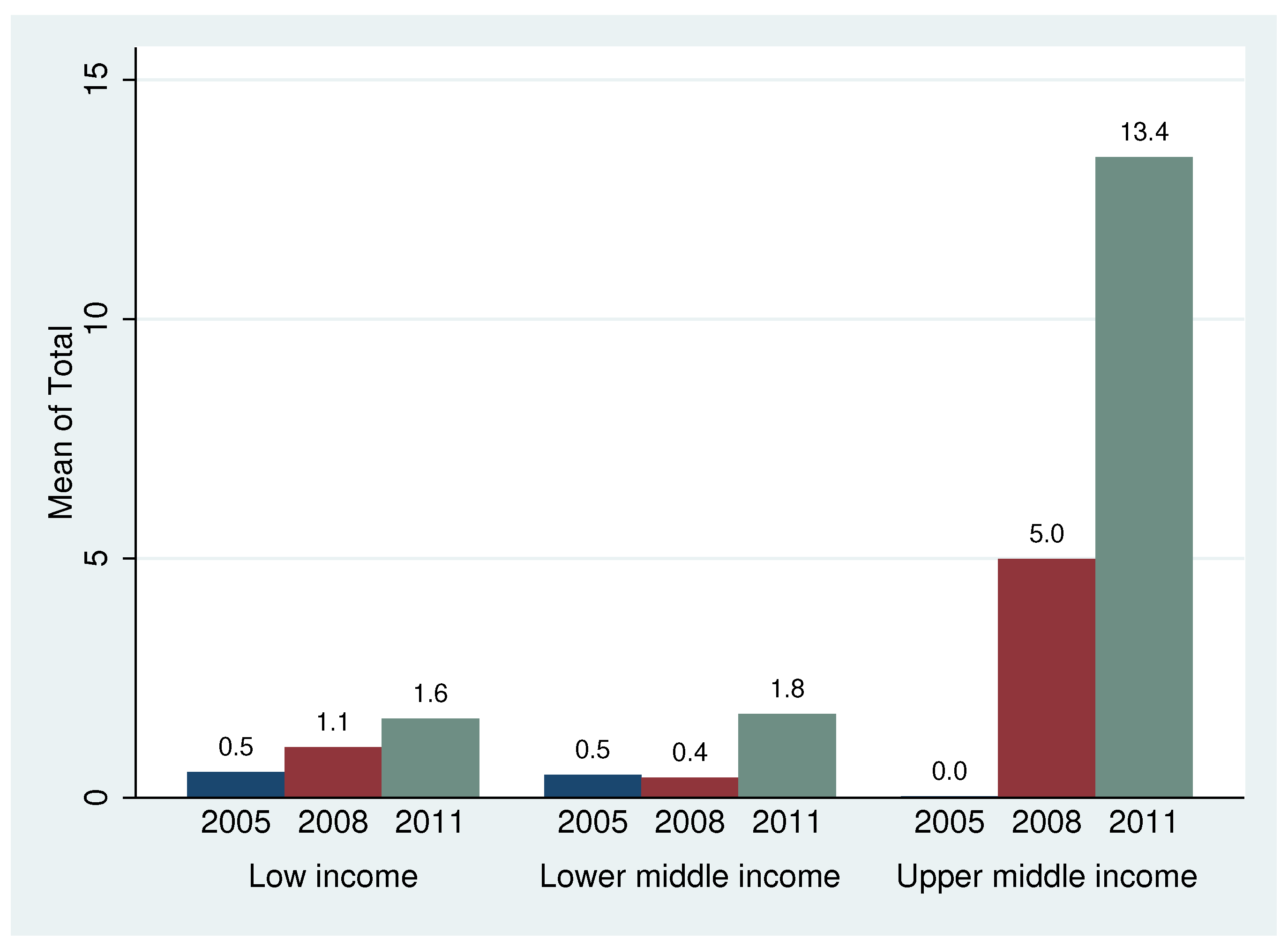
Table 1 illustrates the significant variation in TOTAL across countries. In 2005, microinsurance was offered in 20 countries, growing to 32 in 2008 and 39 in 2011. On average, less than 0.5 percent of the African population was covered by microinsurance in 2005, growing to more than 3.5 percent in 2011. Although microinsurance is still not offered in many countries on the continent, in Namibia and South Africa, more than 50 percent of the population purchased microinsurance coverage in 2011. In Namibia, TOTAL grew from 0 in 2005 to 6.7 percent in 2008 and 57.5 percent in 2011.
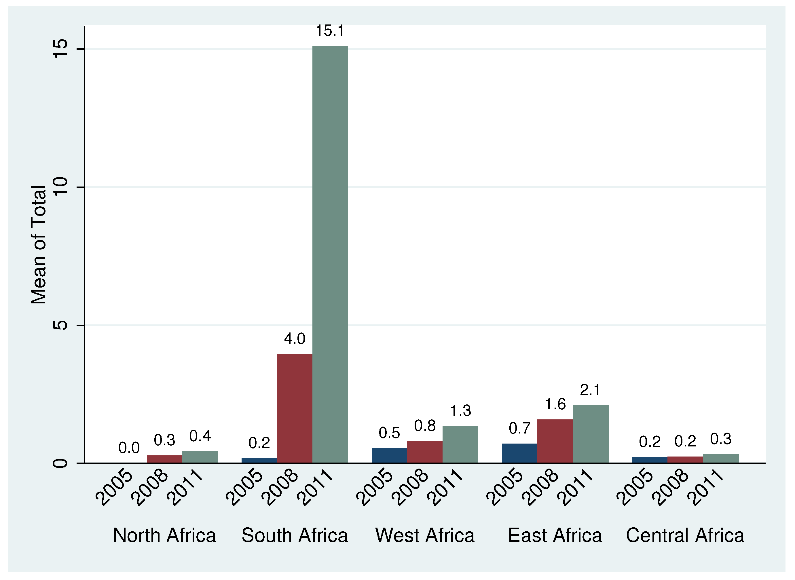
Figure 1 shows the distribution of TOTAL across years and income groups as defined by the World Bank. Microinsurance appears to be more prevalent in upper–middle-income economies, which is driven by the inclusion of South Africa in the censuses of 2008 and 2011 and the explosive growth of microinsurance in Namibia. After excluding these two countries from the sample, the mean of TOTAL exhibits little variation across income groups. However, as
Figure 2 illustrates, TOTAL varies substantially across geographic regions (
Appendix A lists the countries in the sample by regions). Microinsurance is less prevalent in North and Central Africa compared with the rest of the continent. Although not without its limitations, the dataset collected by the MicroInsurance Centre is unique and unmatched by any other existing source in terms of detail and accuracy. For example, the dataset was used by
Biener and Eling (
2011) as “representative market data” (p. 94) in comparison with the authors’ sample for consistency.
4. Empirical Models
Data are used to estimate two empirical models. The aim of the cross-sectional model is to isolate the effect of microinsurance on subsequent economic growth, whereas the panel data model examines the contemporaneous effect of microinsurance on economic growth.
The cross-sectional regression model is expressed as
where
i denotes the country;
represents unobserved country-fixed effects, which vary across countries but do not vary across time; and
is a random error term. The conditioning information set (
) includes country-varying growth determinants, and
,
, and the vector
are the coefficients to be estimated.
A detailed description of the variables and data sources is provided in
Appendix B, whereas in-sample summary statistics and correlations are presented in
Table 1. The dependent variable is the real annual GDP per capita growth. TOTAL, as described in detail in
Section 3, is the microinsurance coverage ratio in 2005.
Determinants of growth identified by other empirical studies are controlled for to isolate the causal effect of microinsurance on economic growth. However, model uncertainty is a fundamental problem of growth regressions (
Temple 1999). According to
Levine and Renelt (
1992), more than 50 variables have been found to be significantly correlated with growth in at least one growth regression. I reference empirical studies on the finance–growth nexus to adopt a parsimonious set of control variables (
Arena 2008;
Levine et al. 2000).
The conditioning information set includes INITIAL GDP, the natural logarithm of real per capita GDP at the start of the period, to capture conditional convergence effects. To capture possible nonlinearities in the microinsurance–growth nexus discussed in
Section 2, a variation in the model is estimated, which introduces an interaction of TOTAL with INITIAL GDP into Equation (
1). Based on theory, the interaction term should enter the regression equation with a negative sign. The conditioning information set (
) also includes human capital at the beginning of the period, as measured by the primary completion rate;
2 the terms of trade growth to control for the international environment; the sum of exports and imports as a share of GDP to control for trade policies; the ratio of M2 to GDP, which was first proposed by
King and Levine (
1993) as a standard measure of the impact of financial liberalization and financial deepening on savings and investment; and government consumption and inflation to account for macroeconomic policies.
3Finally, a measure of institutional quality is constructed as the (arithmetic) average of the aggregate governance indicators constructed by
Kaufmann et al. (
2010). For a large sample of countries,
Kaufmann et al. (
2010) constructed six non-mutually exclusive aggregate governance indicators (government effectiveness, corruption, political stability, regulatory quality, rule of law, and voice and accountability) grouped into two broad categories: the process by which governments are selected, monitored, and replaced and the capacity of government to effectively formulate and implement sound policies.
The microinsurance sector in Africa is one example in which financial innovation has preceded regulation. African countries either do not have regulation pertaining specifically to microinsurance or such regulation is in its nascent stage.
4 Thus, the model does not include a variable that explicitly captures the microinsurance regulatory environment in a country.
Cross-country growth regressions average data over four- or five-year periods to abstract from business cycle effects and focus on long-term growth differences across countries. Using the average of the variables over the available time period has several advantages, such as (1) enabling measurement of the long-run impact of our covariates on net growth of any cyclical factors; (2) reducing the measurement error, which can dominate results when using short-term data (
Barro 1997); (3) smoothing the data, resulting in a better fit; and (4) providing more reliable estimates in cases such as ours, where data are available for a limited number of years, with gaps in the time series (
Beck and Levine 2004).
For each country in the sample, data on GDP per capita growth and terms of trade growth are averaged over the sample period (2005–2011). However, to control for possible endogeneity of the other regressors, they enter into the regression equation with their initial values from 2005. Thus, for each country, there is ideally one observation for each variable to estimate Equation (
1). Using the value of TOTAL at the beginning of the period rather than its average has the added benefit of accounting for the possibility of a delay before the effect of microinsurance is felt in the economy.
The cross-sectional regression method has been the subject of severe criticism (
Islam 2003;
Temple 1999); the major reason being the possibility of omitting country-specific fixed effects. However, cross-sectional growth regressions have an advantage over panel data techniques in that they can produce consistent estimates of the average coefficient, even in a dynamic model, provided that certain preconditions are met. Parameter heterogeneity is of particular concern in cross-country regressions because, according to
Temple (
1999), empirical evidence suggests that widely heterogeneous countries in cross-country regressions exhibit differential responses to a unit change in a control variable. Furthermore, Temple argues that the problem of parameter heterogeneity is more pronounced in dynamic panel data models.
Data for 2005, 2008, and 2011 for a large cross-section of African economies are pooled to estimate the following panel regression model:
where
t denotes the time period. For consistency, the same set of explanatory variables is used as in Model (
1). Except for INITIAL GDP, M2/GDP ratio, and the primary completion rate, which are lagged by one period (three years), the remaining regressors enter the model contemporaneously.
represents time-fixed effects to control for factors that change over time but do not vary across countries, and
is an idiosyncratic disturbance assumed to be uncorrelated across countries.
The major difference between Models (
1) and (
2) is that Model (
2) accounts for a contemporaneous relationship between microinsurance and economic growth, whereas Model (
1) defines an intertemporal relationship. Unobserved heterogeneity across countries is controlled for in both cross-sectional and panel data regressions, and both ordinary least squares (OLS) and two-stage least squares (2SLS) are used to estimate the models. In addition, the lagged values of the regressors are used in cross-country regressions to partially address endogeneity concerns.
5. Econometric Methodologies
Both an ordinary least squares and instrumental variable approach are employed to estimate the contemporaneous and longer-term impact of microinsurance on economic growth, conditional on the regressors in the information set.
Data on the total number of lives and properties covered in Africa are not available for every country in every year, i.e., the panel is unbalanced with a short time dimension but a larger cross section of countries. Several econometric issues have to be addressed when deciding on an identification method. First, one might argue that microinsurance is a passive consequence of growth, i.e., the direction of causality is from growth to microinsurance rather than the other way around. Second, the presence of unobserved or unmeasurable country-specific effects that, if correlated with the explanatory variables and left untreated, lead to omitted variable bias.
I start by addressing the unobserved heterogeneity problem. Theory predicts that differences in initial conditions such as initial efficiency, resource endowments, and institutions affect the steady-state level of output and, therefore, should be controlled for. In growth models, unobserved cross-country heterogeneity is typically assumed to be constant over time and treated as a fixed rather than random effect because of its plausible correlation with one or more of the covariates in the model (
Islam 2003). If left untreated, the fixed effects render the OLS estimates biased and inconsistent, corresponding to one of the criticisms of cross-country growth regressions, which widely ignore unobserved country-specific effects. However, even traditional panel data estimators that control for country-specific effects, such as the fixed-effects estimator, are biased and, in data with limited time dimensions, inconsistent in a dynamic model (
Nickell 1981).
The “Africa dummy” first introduced by
Barro (
1991) has been consistently found to be negative and statistically significant in empirical studies; “failure has been concentrated in sub-Saharan Africa”, notes
Temple (
1999) (
p. 130). The Africa dummy can be thought of as a measure of our ignorance of region-specific factors in sub-Saharan Africa, which can help to explain the dismal growth performance of the region, given its strong economic fundamentals. A number of studies have attempted to open the “black box” of the Africa dummy by proposing a variety of explanations, including geographic factors and trade openness (
Sachs and Warner 1997), government consumption (
Barro 1997), policy differences between sub-Saharan Africa and the rest of the world (
Easterly and Levine 1997), and differences in initial efficiency (
Temple 1999).
However,
Koop et al. (
1995) suggested that more variation exists
across continents than
within continents. Although Africa’s growth performance differs from that of countries with similar fundamentals in the rest of the world, cross-country variation in Africa itself appears to not be as extensive. For example,
Durlauf and Johnson (
1995) examined the possibility of multiple regimes in which heterogeneous groups of countries converge to different steady-state equilibria. Based on output and education in 1960, they used a nonparametric approach to group a large sample of countries into four homogeneous subgroups with a common linear cross-sectional regression equation. All the African countries in their sample except for South Africa and Madagascar fall in two adjacent groups: the low-output/low-literacy group and the intermediate-output/low-literacy group. Therefore, we follow the suggestion of
Griliches and Mairesse (
1995) and
Temple (
1999) to proxy for omitted variables such as initial conditions rather than “purge” the fixed effects (
) through first differencing, for example.
To proxy for time-invariant cross-country heterogeneity, regional dummies for the North, South, East, and Central Africa regions (West Africa serves as the base region) obtained from
Nunn and Puga (
2012) are introduced. The controls are used in both cross-sectional and panel data analyses.
Proxying for unobserved heterogeneity has the added benefit that it maximizes the data sample in panel regressions and enables the use of both within and between variation in the data for identification. Alternatively, if we are to difference the data, a substantial portion of the sample will be lost, because first differencing magnifies gaps in unbalanced panels—a problem that is further exacerbated by the poor data quality in 2008, when a distinction was not made between zero microinsurance and missing data.
To control for possible endogeneity of TOTAL (as well as other regressors) stemming from its joint determination with growth, in cross-sectional regressions, the initial value of TOTAL is used rather than its average. In addition, the instrumental variable approach is used to address the endogeneity problem, whereby the rank order of the observed microinsurance coverage ratio (RANK) is used as an instrument for TOTAL. Countries are sorted by their microinsurance coverage ratio, then assigned a numerical rank calculated in ascending order. Thus, by construction, RANK is positively correlated with TOTAL. In panel data regressions, RANK is calculated for every year of data in the sample. The rank-order instrumental variable approach has been successfully used to address the endogeneity issue in a wide range of economic contexts (
Edwards and Waverman 2006;
Evans and Kessides 1993;
Jones and Jorgensen 2012;
Kroszner and Stratmann 1999;
Rummery et al. 1999).
A priori, RANK is a relevant instrument because, by construction, it should be highly correlated with the observed microinsurance coverage ratio. Furthermore, RANK is an ordinal variable, and as such, the distance between categories does not have any meaning. As long as random factors that can affect both economic growth and microinsurance do not affect the microinsurance rank order of the country, RANK should be uncorrelated with the random error term in the structural equation; that is, as long as the instrument is redundant in the structural equation, i.e., RANK has no effect on growth once the other regressors (including TOTAL) are controlled for, it should also be orthogonal to the random error term in the structural equation. In regressions including the interaction term of TOTAL with INITIAL GDP, RANK, its square, and the interaction of RANK with INITIAL GDP are used as instruments. However, I do not control for possible endogeneity of the remaining regressors in the panel data model, which precludes drawing definite conclusions about causality in panel data analyses.
Two different approaches are used to test for instrument relevance. First, the fit of the first stage regressions is examined using
Shea (
1997)’s partial
, which accounts for intercorrelations among the instruments, to measure the explanatory power of the excluded instruments. In addition,
Kleibergen and Paap (
2006)’s rk LM test, which is robust to heteroscedasticity, autocorrelation, and clustering, is used to assess the strength of identification. The Kleibergen–Paap rk test statistic is used to test the null hypothesis that the structural equation is underidentified, i.e., that the excluded instruments are not relevant, meaning not correlated with the endogenous regressors.
To formally test for the endogeneity of TOTAL and its interaction with INITIAL GDP, the difference-in-Hansen J test or C statistic is used rather than the more conventional Durbin–Wu–Hausman test, because the Durbin–Wu–Hausman test is not robust to heteroscedasticity. Under the null hypothesis that the endogenous regressors can be treated as exogenous, the C statistic follows the chi-squared distribution with degrees of freedom equal to the number of regressors tested.
The instrumental variable approach is used for estimation rather than the more general and efficient generalized method of moments (GMM) because of the well-known poor small-sample properties of GMM.
Baum et al. (
2003), among others, advise that instrumental variable estimation is preferable to efficient GMM when the error terms in the structural Equation (
2) are homoscedastic. The test for heteroscedasticity proposed by
Pagan and Hall (
1983) is used to ascertain that the error terms in all instrumental variable regressions are homoscedastic.
Alternative estimators for linear dynamic panels with fixed effects are the difference and system GMM, which have gained popularity in recent empirical work on economic growth. The difference GMM estimator developed by
Holtz-Eakin et al. (
1988) and
Arellano and Bond (
1991), popularly known as the “Arellano–Bond” estimator, and the more robust and efficient “Blundell–Bond” estimator conceptualized by
Arellano and Bover (
1995) and formalized by
Blundell and Bond (
1998), produce consistent estimators in the presence of fixed effects and endogenous regressors (
Roodman 2009 offers an excellent discussion). One of the advantages of the difference and system GMM estimators is that they can tackle the endogeneity problem, which plagues the growth literature. Further, numerous instrumental variables are available from within the system, depending on the stringency of the assumptions one is willing to make, without sacrificing sample size, representing a formidable advantage, given the paucity of suitable instruments in growth regressions. However, based on some of the most influential growth studies,
Bazzi and Clemens (
2013) illustrated that such instruments are “blunt”. In many cases, they explain only a negligible fraction in the variation in the endogenous explanatory variables. Bazzi and Clemens state “weak instruments may generate spurious findings in important applications, especially those using the popular Generalized Method of Moments (GMM) dynamic panel estimators” (p. 152).
However, formal tests for instrument strength in dynamic panel GMM regressions do not presently exist. Furthermore,
Temple (
1999) casts doubt on the exogeneity of such internal instruments. He notes that the effect of a factor such as human capital accumulation may take a long time to be felt in the economy; therefore, the lagged difference in human capital may not be a valid instrument for its contemporaneous value. Such an issue is of particular concern in the context of the present work, which considers only three time periods. At least four periods are required to perform the
Arellano and Bond (
1991) test for autocorrelation in the error terms to confirm that all lags of the endogenous variables are valid instruments.
Hansen and Tarp (
2001) argue that in such cases, the instrumental variable estimator might be less biased than the GMM estimator.
The possible impact of the relatively short time series dimension of the data on the results also needs to be considered. One might argue that fewer than 10 years of data may be insufficient to estimate the impact of microinsurance on long-run growth, particularly if microinsurance affects growth with a long lag. Furthermore, using short time series can lead to results being dominated by measurement error (
Barro 1997) or hypothesis tests having low power (
Temple 1999). However,
Clemens et al. (
2012) note that the debate about the use of short versus long periods to measure the impact of a variable of interest on long-run growth has not been resolved. The authors illustrated that in some cases, even a twenty-year time series may not be sufficiently long.
Using longer data series has its drawbacks as well. First, the sparse data on African countries make construction of a balanced panel impossible over a long period. Secondly, although a long time series of data increases the precision of the estimates, it also makes it more difficult to isolate the causal effect of a variable of interest on economic growth, owing to the effect of the numerous random factors that affect economic performance over the long run. Over time, variability in growth most likely increases relative to the variability in microinsurance, making it difficult to find a statistically significant effect of microinsurance on growth. Thirdly, a longer time series poses a threat of omitted variable bias. Finally, microinsurance as we know it has been in existence for only a couple of decades. Despite the data and model limitations, this research has a role to play in shedding light on the macroeconomic impact of such a novel development phenomenon.
6. Results: Intertemporal Relationship
First, the model is estimated without microinsurance. The results reported in column (1) of
Table 2 indicate that all variables have the expected sign, most of them are statistically significant at conventional levels, and the model explains 25 percent of the variation in GDP growth. The negative and statistically significant sign of the initial value of per capita GDP captures the conditional convergence effect. Ceteris paribus, financial intermediary development has a sizable and statistically significant positive effect on subsequent economic growth, whereas, as expected, inflation has an economically and statistically significant negative effect on growth. The large and highly significant positive coefficient of the terms of trade growth indicates that in Africa, an improvement in terms of trade is followed by either an enhanced employment factor or enhanced productivity (
Barro 1997). Despite having the expected sign, the coefficients of the primary completion rate, government consumption, and institutional quality do not have a statistically significant effect on growth. Once the measure of microinsurance is introduced to the standard growth model, estimates using both OLS and 2SLS (column (2) of
Table 2) indicate that TOTAL has a positive although statistically insignificant effect on growth.
To test for nonlinearities in the microinsurance–growth nexus, a variation in the model is estimated in which both TOTAL and its interaction with INITIAL GDP are included. The results are presented in column (3) of
Table 2. The coefficients of TOTAL and its interaction with INITIAL GDP are large in magnitude and statistically significant at conventional levels using both OLS and 2SLS. The low
p-value of the difference-in-Hansen test statistic reported at the bottom of column (3) indicates that TOTAL and its interaction with INITIAL GDP cannot be treated as exogenous; therefore, instrumental variable estimates should be relied upon for inference.
The first-stage Shea’s partial
indicates that the excluded exogenous variables, RANK and its square, explain a significant portion of the variation in TOTAL and its interaction with INITIAL GDP for all estimates presented in
Table 2. The Kleibergen–Paap rk LM test for instrument relevance confirms that the instrumental variables are strong, whereas the Hansen J test of overidentifying restrictions confirms that they satisfy the exclusion restriction, lending support to the estimates.
The results presented in column (3) indicate that the exogenous component of microinsurance has a sizable and statistically significant effect on subsequent economic growth. The level of microinsurance in 2005 predicts GDP growth over the subsequent seven-year period after controlling for a large set of country characteristics. The marginal effect of microinsurance is a negative function of initial output, implying that microinsurance has a differential impact on economic growth contingent on the country’s initial level of development. The impact is larger in countries with a lower standard of living. Using the instrumental variable estimates reported in column (3) of
Table 2, the threshold income level at which the effect of microinsurance changes from positive to negative is about USD 460 (constant 2005 US dollars). About 40 percent of the countries in the sample have a starting GDP level lower than this threshold.
For example, Niger did not have microinsurance in 2005, whereas the mean value of TOTAL in the sample was about 0.5 percent. Using 2SLS, the marginal effect of microinsurance on economic growth evaluated at Niger’s initial value of GDP (in natural logarithm) (5.55) is statistically significant at 1.14, which implies that an exogenous change in microinsurance that had pushed Niger to the sample mean value would have accelerated its subsequent annual growth rate by about 0.6 percentage points. If, instead, 2 percent of Niger’s population were covered by microinsurance, its annual growth rate over the next seven years would have averaged about 0.9 percent rather than the actual −1.4 percent, illustrating the economically significant impact of microinsurance in low-income countries. However, this hypothetical exercise does not provide any guidance with respect to how such an “exogenous change” in microinsurance can be initiated.
6.1. Robustness Checks
In the sections below, the results are subjected to a number of robustness checks to ascertain their validity.
6.1.1. Influential Observations
Easterly (
1995) argues that the results of many growth regressions are driven by outliers. The measure suggested by
Belsley et al. (
1980), DFBETA, is used to identify influential observations that have a particularly large impact on regression coefficients. DFBETA is measured by the difference (in absolute value) in the regression coefficient of interest when an observation is included and excluded from the model scaled by the estimated standard error of the coefficient. The commonly used cutoff value of 1 is adopted to identify influential observations (an observation is considered influential if it increases the coefficient of any regressor by more than one standard deviation).
Using DFBETA, Senegal has a considerable impact on the coefficients of TOTAL and its interaction with INITIAL GDP. Angola has a sizable impact on the coefficient of government consumption, while Zimbabwe has a considerable effect on inflation.
Table 3 reports the results of rerunning the regressions without these observations. The coefficient estimates of the variables of interest and their standard errors suggest that dropping the influential observations strengthens the correlation between microinsurance and economic growth. As expected, the explanatory power of all regressions without outliers is increased, as indicated by the increased adjusted
s in the OLS regressions. Identification remains strong, as indicated by the low
p-values of the Kleibergen–Paap LM test and the high Shea’s partial
values reported in
Table 3. The 2SLS models pass the Hansen test of overidentifying restrictions, suggesting that the relationship between microinsurance and growth cannot be attributed to simultaneity bias. The low
p-values of the difference-in-Hansen test indicate that we can reject the null hypothesis that the suspect endogenous variables can be treated as exogenous. The Pagan–Hall test fails to reject the null hypothesis of no heteroscedasticity in all 2SLS regressions, suggesting that the instrumental variable approach is preferable to efficient GMM.
The OLS estimates reported in column (4) indicate that once the influential observations are excluded, TOTAL has a large positive and statistically significant impact on subsequent economic growth in the linear model. However, this impact is insignificant in the 2SLS regression. Although we cannot discard the OLS results as spurious, the low p-value of the difference-in-Hansen test suggests that the OLS estimates are inconsistent and that their standard errors are unreliable.
Column (5) of
Table 3 presents regression estimates of the model, which include both TOTAL and its interaction with INITIAL GDP. A comparison with column (3) of
Table 2 suggests that the full-sample estimates are robust to the exclusion of influential observations. Whereas the coefficient estimates of TOTAL and its interaction with INITIAL GDP change quantitatively compared with the estimates using the full sample, they become more statistically significant and the implications are qualitatively the same; ceteris paribus, microinsurance has a large, positive, and statistically significant impact in low-income economies. However, the threshold value of INITIAL GDP at which the effect of TOTAL changes sign from positive to negative is somewhat lower, at about USD 340; only about 25 percent of the countries in the subsample without outliers fall below this threshold level.
6.1.2. Additional Controls
The robustness of the results presented in
Table 2 is also tested by augmenting the conditioning information set, with a large array of explanatory variables found to account for cross-country growth differences in other studies. For brevity, results are not presented here but are available from the author upon request. Overall, adding regressors to the control set one at a time does not quantitatively change the regression estimates presented in
Table 2.
The notion of a “resource curse” (
Auty 1993) has become synonymous with Africa. The abundance of natural resources in sub-Saharan Africa has been paradoxically blamed for the dismal growth performance of the continent. To test for the resource curse, I include GEMSTONES, the total amount of gem-quality diamonds extracted over the period of 1958–2000 measured in 1000 carats obtained from
Nunn and Puga (
2012), and rerun the regressions reported in
Table 2. Results indicate that including this measure of natural resource abundance does not qualitatively alter the effect of microinsurance on economic growth, whereas the effect of GEMSTONES is not statistically significant at conventional levels in any regression. The results are also robust to the inclusion of LATITUDE and TROPICAL, which are proxies for a tropical climate (see
Bloom and Sachs 1998) in the conditioning information set. The reported results should not be taken as evidence of the lack of a resource curse or a lack of support for the “geography hypothesis”. Such geography measures are found to be insignificant
after controlling for the variables in the conditioning information set.
Hall and Jones (
1999) and
Rodrik et al. (
2004) argue that the effect of geography on economic growth is mediated by institutions, which I control for.
Easterly and Levine (
1997) argue that the high ethnic diversity in Africa, a legacy of its colonial past, contributes to what the authors call “Africa’s growth tragedy”. However, their measure of ethnic diversity (ETHNIC) is statistically insignificant at conventional levels in all regressions. One plausible explanation is that, as Easterly and Levine suggest, ETHNIC retards economic growth through its effect on public policy, which is controlled for. However, ETHNIC is also insignificant if the average growth rate is regressed on ETHNIC alone. Another plausible explanation is that ETHNIC is less variable within Africa than among the more diverse pool of countries in Easterly and Levine’s sample, leading to the imprecise estimate of its impact on economic growth in the African sample. Thus, whereas ETHNIC may explain why the growth performance of African countries differs from that of comparable economies in the rest of the world, in this sample, it fails to explain intracontinental differences in growth performance in Africa.
The results are also robust to the inclusion of life expectancy or fertility rate in the control set. Using SCHOOL, which represents the average years of schooling from the dataset of
Barro and Lee (
2013), as a measure of education rather than the primary completion rate reduces the full sample to 33 countries. However, the results are qualitatively the same. The coefficient of SCHOOL is insignificant at conventional levels in all regressions, suggesting that our quantitative measures of education probably do not reflect the quality of education. Literacy surveys in Africa and elsewhere indicate that a large share of adults who have completed primary school are practically illiterate and innumerate (
Glewwe 2002). As a result, many authors argue that education quality is more important than quantity as measured by the primary completion rate or years of schooling with respect to economic growth (
Barro 1997;
Hanushek and Kimko 2000). However, comprehensive and reliable internationally comparable data on quantitative measures of educational quality for Africa are not available.
7. Results: Contemporaneous Relationship
Table 4 presents the results of Equation (
2) estimated using panel data for 2005, 2008, and 2011 on a cross-section of African countries. Data for 2002, 2005, and 2008 are used for variables that enter the regression equation with their initial values (INITIAL GDP, M2/GDP, and primary completion rate). Cluster-robust standard errors (
Arellano 1987), which account for both heteroscedasticity and correlation of observations
within a country, are reported in parenthesis.
The higher frequency of data affects both the coefficient estimates and the explanatory power of the regressions. No first-order serial correlation is observed in the residuals from the pooled OLS regressions, suggesting that the heterogeneity bias is successfully addressed by adding regional indicators to the model. Furthermore, the Pagan–Hall test fails to reject the null hypothesis of no heteroscedasticity for any instrumental variable regression, suggesting that the instrumental variable approach is preferable to efficient GMM.
Similarly to cross-sectional regressions, the primary completion rate is statistically insignificant, whereas the terms of trade growth and the M2/GDP ratio are statistically significant at conventional levels in all regressions. In contrast, openness to trade, institutions, and government consumption, which are insignificant in cross-country growth regressions, are statistically significant at conventional levels and with the expected sign in panel data regressions. Government consumption has a negative sign, in line with the view that it does not enhance the productive capacity of the economy.
The difference-in-Hansen test indicates that we can treat TOTAL and its interaction with INITIAL GDP as exogenous in all regressions. Therefore, the focus is on the OLS estimates, which are more efficient than the 2SLS estimates. Column (7) of
Table 4 suggests no evidence of a linear contemporaneous relationship between microinsurance and growth in the sample. The coefficient of TOTAL is small and positive but statistically insignificant at conventional levels.
Results of the regression including both TOTAL and its interaction with INITIAL GDP are presented in column (8). Both TOTAL and its interaction with INITIAL GDP are statistically significant at the 10 percent level. The threshold level of INITIAL GDP per capita at which the marginal effect changes sign from positive to negative is about USD 4600, implying that for an overwhelming majority of the countries in the sample, the marginal effect of microinsurance on contemporaneous economic growth is positive. While definite conclusions about causality cannot be drawn, the results suggest that the development of the microinsurance market predicts an increased contemporaneous growth rate across the countries in the sample after controlling for differences in macroeconomic policies, institutions, and education, as well as the international environment. The robust effect of microinsurance on economic growth in both cross-sectional and panel data regressions after controlling for the M2/GDP ratio suggests that microinsurance conveys information in addition to financial development, emphasizing the unique role of the insurance sector as a provider of risk transfer and indemnification in the economy.
For low-income economies, the partial derivative of growth with respect to TOTAL is smaller in panel data regressions than in the corresponding cross-sectional regressions, implying that in such economies, the effect of microinsurance on economic growth is smaller on impact than its subsequent effect on growth. Let us consider the example of Niger again. Niger did not have microinsurance in 2005, whereas the mean value of TOTAL in the dataset was about 0.5 percent. The marginal effect of microinsurance on economic growth evaluated at Niger’s value of GDP in 2002 (in natural logarithm) (5.57) is 0.51. The effect is statistically significant at the 10 percent level. An exogenous change in microinsurance, which pushed Niger to the sample mean value, would have accelerated its annual growth rate on impact by about 0.25 percentage points. Although this contemporaneous effect of microinsurance is nontrivial, it is significantly lower than its intertemporal effect of 0.6 percentage points discussed in
Section 6.
Table 5 illustrates that the results are not driven by influential observations. Using DFBETA, I exclude the 2005 observation of Ethiopia from the sample, which has a large impact on the coefficient of inflation, and rerun the regressions. The difference-in-Hansen test suggests that we can continue to rely on the OLS estimates. Excluding the single influential observation from the full sample affects the coefficient of inflation, which changes from negative to positive, despite remaining statistically insignificant; however, this result does not change the coefficient estimates presented in
Table 4 in any substantial way.
The results presented in
Table 4 are also robust to appending the conditioning information set to include ETHNIC, life expectancy, fertility rate, gemstones, or tropical climate. These sensitivity results are not presented here for brevity, but they are available upon request from the author.
8. Nonlinearities in the Microinsurance–Growth Nexus
The results suggest that microinsurance has an overwhelmingly positive effect on economic growth in the immediate period. However, over time, whereas the impact of microinsurance remains positive in the poorest economies, it can be insignificant and possibly even negative in higher-income economies. This nonlinear effect is consistent with the theoretical literature and related empirical studies discussed in
Section 2. However, all countries in the sample are developing economies (classified as low- and middle-income economies by the World Bank), which may be expected to benefit from the development of the microinsurance sector.
To understand the relationship between economic growth and microinsurance in the nonlinear model and how this relationship changes over time, the marginal effect of microinsurance is computed, and its statistical significance is evaluated at different values of INITIAL GDP. The 2SLS estimates are used to compute the partial derivative of growth with respect to TOTAL in the cross-sectional regression model and the OLS estimates for the panel data model.
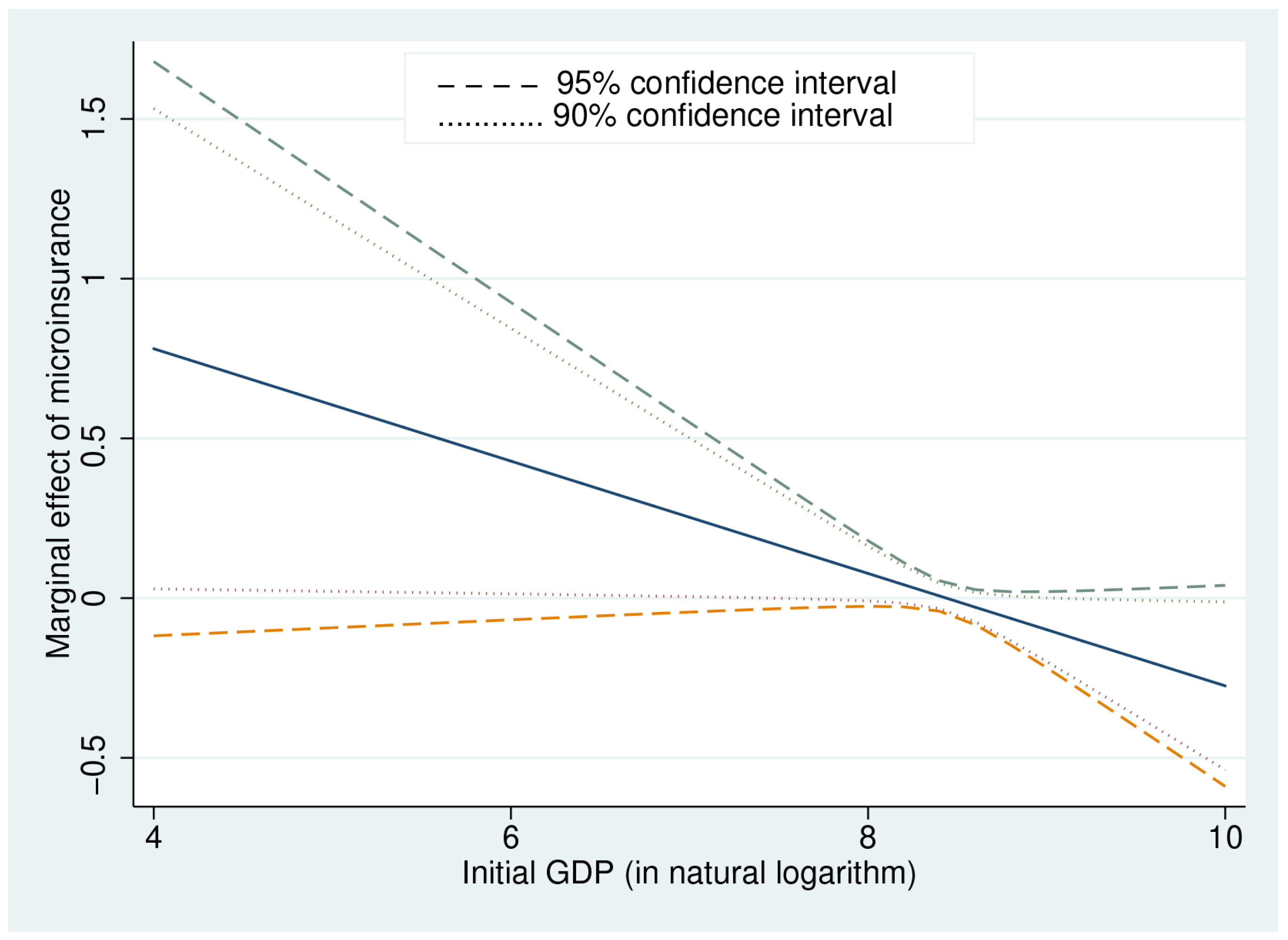
Figure 3 depicts the intertemporal marginal effect of microinsurance on economic growth, as well as the 90- and 95-percent confidence bounds evaluated at different values of INITIAL GDP using the full sample. The partial effect of TOTAL on economic growth decreases with INITIAL GDP. The turning point at which the marginal effect changes from positive to negative is about USD 460 in the full sample (USD 340 in the sample without outliers), which is well within the sample range. For the full sample,
Figure 3 illustrates that the marginal effect is positive and statistically significant at the 10 percent level for INITIAL GDP values of less than about USD 310. Only eight countries in the sample have such low values of INITIAL GDP. The marginal effect becomes significantly negative at the 10-percent level for values of INITIAL GDP greater than USD 3000. Only five countries or about 13 percent of the countries in the sample have such a high starting level of GDP. However, at the five-percent level, the marginal effect of microinsurance is never statistically significant for the range of values of INITIAL GDP in the sample.
Figure 4 shows that the results cannot be attributed to influential observations. An evaluation of the partial derivative of GDP growth with respect to TOTAL after excluding the influential observations identified in
Section 6 shows that the marginal effect of microinsurance is positive and statistically significant at the 5-percent level for fewer than 20 percent of the countries in the sample and negative and statistically significant for more than 50 percent of the countries.
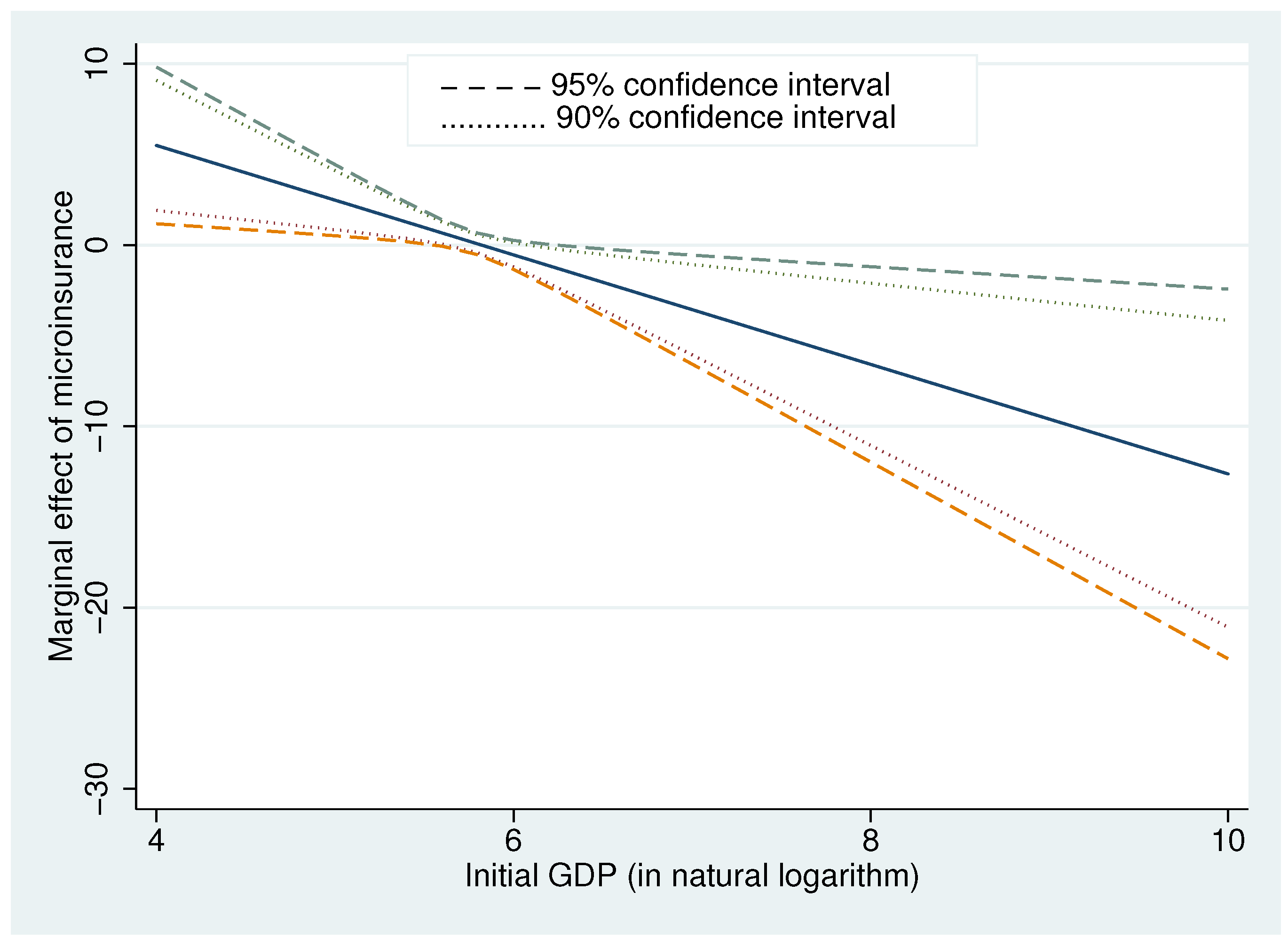
Turning to the panel data,
Figure 5 depicts the marginal effect of microinsurance on contemporaneous economic growth for countries with different levels of development estimated based on the full sample. Results for the sample excluding the single influential observation identified in
Section 4 are omitted without loss of generality. The marginal effect is positive and significant at the 10-percent level for the majority of the countries in the sample. The marginal effect is negative and statistically significant for only a single country at the 10-percent level. However, at the 5-percent level of significance, the marginal effect, whether positive or negative, is insignificant for the range of values of INITIAL GDP considered in this study.
In summary, the results suggest that ceteris paribus, microinsurance has a strong positive and contemporaneous effect on economic growth for an overwhelming majority of the countries in the sample. The marginal effect of microinsurance on subsequent economic growth is larger in magnitude, positive, and statistically significant for low-income economies. However, the positive effect diminishes quickly with the level of development and may be nonexistent or even negative (depending on the level of significance one is willing to adopt) in countries with a higher level of development. The significant negative partial derivative of growth with respect to TOTAL at relatively low starting values of GDP in cross-sectional regressions is puzzling, because it suggests that whereas microinsurance has an overwhelmingly positive effect on growth, it may fail to leave a lasting trace on the economy in some developing economies.
One plausible explanation is that not all microinsurance products are “created equal” in terms of their impact on economic growth. By aggregating microinsurance products, we ignore the possibility that some products do enhance economic growth significantly, whereas others have only a marginal or no impact on economic growth. For example, based on panel data on developing and developed economies,
Arena (
2008) found that both life and nonlife insurance products enhance economic growth. However, using a linear model, he also found that life insurance premiums are not growth-enhancing in developing countries, whereas nonlife insurance premiums have a positive effect on economic growth in both developing and developed economies. Arena’s findings are supported by the results reported by
Han et al. (
2010), who found that both life and nonlife insurance are growth-enhancing in developing countries but that nonlife insurance appears to have a larger positive impact on economic growth.
To confirm this supposition more rigorously, I disaggregate the measure of microinsurance into life (LIFE) and nonlife (NONLIFE) microinsurance, as defined by the OECD. LIFE and NONLIFE measure the total number of lives and properties covered under life and nonlife microinsurance products, respectively, in 2005. Then, the cross-sectional model is estimated separately for life and nonlife microinsurance.
Table 6 shows the results. Estimation results of the effect of the aggregate measure of microinsurance on economic growth are also provided as a reference.
The linear model predicts that life microinsurance has a larger effect on economic growth than nonlife microinsurance. However, the effect of nonlife microinsurance is not statistically significant, whereas the statistical significance of life microinsurance is not robust to the estimation method.
In the nonlinear model, life microinsurance, as well as its interaction with INITIAL GDP, does not have a statistically significant effect on economic growth. In contrast, NONLIFE does have a statistically significant effect on growth, conditional on the level of economic development. Whereas the effect of nonlife microinsurance on growth tapers off more slowly than the effect of the aggregate measure of microinsurance and is positive for half of the countries in the sample, the turning point at which the effect changes from positive to negative remains within the sample range. These findings imply that policy makers in low-income economies should encourage the development of the nonlife microinsurance sector, which, at a low level of development, has a more lasting impact on economic growth than nonlife insurance.
9. Conclusions
Over the last decade, international organizations and donors have actively fostered the growth of the microinsurance market in developing nations throughout the world. Despite empirical evidence for the positive microeconomic impact of microinsurance, the broader question of whether inclusive insurance can be used as a vehicle for economic growth remains. The purpose of this study is to take the first steps in understanding the microinsurance–growth nexus based on a rich set of longitudinal data for African countries.
Estimates suggest that microinsurance has a measurable, robust, and statistically and economically significant effect on economic growth, both contemporaneously and intertemporally, after controlling for a large set of country characteristics. The microinsurance–economic growth relationship is best described by a nonlinear relationship. The marginal effect of microinsurance, both contemporaneous and intertemporal, is a decreasing function of the starting level of economic development, as measured by the initial level of real GDP per capita.
Microinsurance has a robust and statistically and economically significant positive effect on economic growth for an overwhelming majority of the countries in the sample, with a greater impact for poor countries. The marginal effect of microinsurance on subsequent economic growth is larger in magnitude (for a given level of development), positive, and statistically significant at conventional levels for countries with a low starting level of development. However, the positive effect tapers off quickly with an increase in the initial level of output. Thus, microinsurance may fail to leave a lasting trace on the aggregate economy in “richer” developing countries. One possible explanation for this finding is that life and nonlife microinsurance have a differential impact on economic growth. In the sample at hand, life microinsurance fails to leave a lasting impact on economic growth, whereas the impact of nonlife microinsurance is lasting and tapers off more slowly with development compared with life microinsurance. From a policy perspective, the reported findings suggest the importance of developing the nonlife segment of the market, which is currently dominated by life microinsurance products.


