Article

Discretionary Extensions to Unemployment Insurance Compensation and Some Potential Costs for a McCall Worker

Department of Economics, California State University, 9001 Stockdale Highway, Bakersfield, CA 93311, USA
Risks 2023, 11(10), 171; https://doi.org/10.3390/risks11100171
Submission received: 19 August 2023 / Revised: 22 September 2023 / Accepted: 27 September 2023 / Published: 28 September 2023

Abstract

:
Unemployment insurance provides temporary cash benefits to eligible unemployed workers. Benefits are sometimes extended by discretion during economic slumps. In a model that features temporary benefits and sequential job opportunities, a worker’s reservation wages are studied when policymakers can make discretionary extensions to benefits. A worker’s optimal labor-supply choice is characterized by a sequence of reservation wages that increases with weeks of remaining benefits. The possibility of an extension raises the entire sequence of reservation wages, meaning a worker is more selective when accepting job offers throughout their spell of unemployment. The welfare consequences of misperceiving the probability and length of an extension are investigated. Properties of the model can help policymakers interpret data on reservation wages, which may be important if extended benefits are used more often in response to economic slumps, virus pandemics, extreme heat, and natural disasters.

1. Introduction

Each month, millions of workers lose their jobs. Unemployed workers search for jobs by answering online adverts, contacting employers, using the services of employment agencies, and asking friends and relatives about employment opportunities. Workers understand the the types and frequency of job offers they expect to receive. Depending on how long they are unemployed, workers are entitled to unemployment insurance compensation, typically 26 weeks. Upon receiving a job offer, a worker has the option to reject the offer and continue their search or accept the job. A sequence of reservation wages describes optimal choices: any wage offer above the reservation level should be accepted. As more weeks of unemployment are endured, and fewer weeks of unemployment insurance remain, the reservation wage will fall, indicating that workers are less selective as benefits expire. Less is known about optimal decisions, however, when policymakers can extend benefits by discretion.
In brief, here is the main issue: Unemployed workers are often entitled to claim 26 weeks of UI compensation. In periods of economic distress, policymakers sometimes extend the number of weeks an individual might claim UI compensation by discretion. When a worker misperceives the probability and length of an extension, what are the costs?
I answer the question from a worker’s perspective. Imagine that Sonia is unemployed and submitting her resume to online adverts. Each week, Sonia receives a job offer that she can accept or reject. Meanwhile, her unemployment compensation benefits are expiring. Between job offers, however, there is a chance that benefits are extended. An extension would allow Sonia to claim additional weeks of UI compensation. If an extension is likely, then Sonia can reject low-wage offers, knowing that her search will likely be supported by extended UI compensation. Sonia’s reservation wage increases. Sonia, though, might not know the true probability that benefits are extended and the length of the extension.
I am interested in Sonia’s welfare costs when she misperceives the probability and length of an extension. If Sonia believes an extension is unlikely to happen, so the true probability of an extension is higher than what Sonia believes, then Sonia risks accepting job offers she would like to reject. In this scenario, if Sonia knew the true probability, then, on average, she would like to spend more time searching in order to find a higher-paying job. To understand these costs, I develop a formal dynamic model of sequential job search with expiring UI benefits, which allows for the possibility that benefits are extended. Burdett (1979) studied expiring benefits in McCall’s (1970) environment of sequential job search. I add to this environment the possibility that benefits are extended. I show how perceptions about the possibility of an extension affect reservation wages, which determine a worker’s job-acceptance criteria.
The decision-making environment I consider captures some features of UI extensions made during and after the Great Recession and the COVID-19 pandemic. For example, extensions to UI compensation benefits created by Congress during the Great Recession under the Emergency Unemployment Compensation program expired three times, and each time Congress had to reauthorize the program to the previous expiration date (Rothstein 2011). In fact, temporary additional UI benefits have been created by Congress nine times: in 1958, 1961, 1971, 1974, 1982, 1991, 2002, 2008, and 2020. These policies have extended the number of weeks a worker could claim UI compensation anywhere from 6 to 53 weeks (Whittaker and Isaacs 2022). As I document in Section 2, there is much uncertainty and risk from a worker’s perspective when extensions are made by discretion.
Because discretionary extensions made to UI compensation benefits are endogenous by design, making econometric work challenging, there is scope for investigating a theoretical model. I present the model in Section 3 and Section 4. Section 5 presents a numerical example. The exercise is not meant to be definitive. Instead, it is meant to demonstrate the theoretical properties established in Section 3 and Section 4. Nevertheless, it is worth noting that the welfare calculations imply small costs to misperceiving benefit extensions. Finding small costs is discussed in the context of the literature in Section 6. Section 7 concludes.

2. Two Episodes of Extended Benefits

There are two ways for UI compensation benefits to be extended: automatically and by discretion. Benefits are automatically extended through the Extended Benefits (EB) program of the UI system. The UI system is a joint federal–state partnership, essentially with 53 different systems (the 50 states, Puerto Rico, the District of Columbia, and the US Virgin Islands). Regular UI in most states provides 26 weeks of UI compensation. The EB program extends the number of weeks a worker can claim UI compensation by 13 or 20 weeks when state-specific unemployment-rate triggers are reached. But, “in practice, the required EB trigger is set to such a high level of unemployment that the majority of states do not trigger onto EB in most recessions” (Whittaker and Isaacs 2022, pp. 1–2). In response, Congress often temporarily extends UI benefits, like they recently did under the Coronavirus Aid, Relief, and Economic Security Act (CARES Act) during the COVID-19 pandemic and the Emergency Unemployment Compensation (EUC) program during the Great Recession (Fujita 2010). From a worker’s perspective, both types of extensions involve uncertainty and risk: Automatic extensions require a forecast of unemployment-rate statistics and discretionary extensions require a forecast of legislative action.1
Details of the EUC program and CARES Act justify investigating the costs associated with misperceiving the probability and length of an extension. Section 2.1 considers a thought experiment about how difficult it was for a worker to perceive that they would be entitled to claim up to 99 weeks of UI benefits after the Great Recession. Section 2.2 shares an index of Google searches for “unemployment benefits extension,” which spikes around potential cutoffs to extended benefits after the COVID-19 pandemic. Both episodes document the significant uncertainty a worker must manage when making decisions about accepting job offers when benefits can be extended.

2.1. Extensions Created in Response to the Great Recession

Imagine that Vernon lived in California and became unemployed in early January 2010 when the United States was dealing with the fallout from the Great Recession. The EB program in California had been triggered on since 22 February 2009, so Vernon could expect to receive 26 regular weeks of UI coverage and 20 EB weeks, for a total of 46 weeks—as long as California did not trigger off its extended-benefits thresholds, requiring Vernon to forecast unemployment-rate statistics. At that time, Vernon could reasonably expect to receive no temporary benefits because the EUC program was set to expire in late February 2010 (Rothstein 2011, p. 150, Table 1). Around 25 weeks later, or around 27 June 2010, California’s EB program had triggered off and the federal EUC program had also expired.2
What Vernon expected then is unknowable, but by 25 July 2010, the EB program had triggered on in California and the EUC program had been reauthorized. Vernon, at that time, could reasonably expect—in addition to the 26 weeks of regular UI compensation just received—20 EB weeks plus 20 + 14 + 13 + 6 = 53 weeks of UI compensation under the four tiers of the reauthorized EUC program (where some of the compensation would be paid retroactively) (Rothstein 2011, p. 153). In total, Vernon could have received up to 26 + 20 + 53 = 99 weeks of UI compensation. Yet, the 99 weeks belies the uncertainty and risk faced by Vernon.3
Vernon’s predicament was pointed out by Kahn (2011) in the context of UI extensions in the aftermath of the Great Recession. After the EUC program was authorized in June 2008, temporary extensions were enacted and reauthorized by Congress in “fits and starts” (Rothstein 2011, p. 149). “For much of the program’s history, the expiration date was quite close. Indeed, on three occasions … Congress allowed the program to expire. Each time, Congress eventually reauthorized it retroactive to the previous expiration date” (Rothstein 2011, p. 150).

2.2. Extensions Created in Response to the COVID-19 Pandemic

Uncertainty similarly surrounded CARES Act extensions. The CARES Act was created by Congress in response to the recession caused by the COVID-19 pandemic. Two CARES Act programs extended UI compensation benefits. The Pandemic Emergency Unemployment Compensation (PEUC) program provided additional weeks of federally funded benefits similar to the EUC program in the Great Recession. And the Pandemic Unemployment Assistance (PUA) program expanded coverage to individuals who would be ineligible for UI benefits (the self-employed, independent contractors, gig-economy workers) and to individuals unemployed due to COVID-19-related reasons. Both programs were reauthorized multiple times. Data on internet searches suggest that workers were concerned about access to extended benefits throughout 2020 and 2021.
Figure 1 depicts a weekly index of Google searches for “unemployment benefits extension.” In early 2020, before the COVID-19 pandemic, the index was near zero. Google searches began rising by mid-March and peaked locally in the week after 27 March 2020, which coincided with the signing of the CARES Act into law, creating “several temporary, now-expired UI programs” (Whittaker and Isaacs 2022).
During the third week of June 2020, the index was around 25. But, when the additional USD 600-per-week benefit created by the Federal Pandemic Unemployment Compensation (FPUC) program expired in the week ending 25 July 2020, the indexed neared its global peak. The 100 peak was reached in the week of 8 August 2020, when President Donald Trump authorized the USD 300-per-week Lost Wages Assistance benefit.
A little over 21 weeks passed between 13 March 2020 (when a nationwide emergency was declared) and 8 August 2020.4 So, up to this point, many workers would have been covered by 26 weeks of regular UI benefits. The local peaks that follow have to do with benefit extensions. In the week of 27 December 2020, the Continued Assistance Act was signed into law, which increased the maximum number of PEUC weeks from 13 to 24 and increased the maximum number of PUA weeks from 39 to 50. In the week of 11 March 2021, the American Rescue Plan increased the maximum number of PEUC weeks to 53 and increased the maximum number of PUA weeks to 79. Both the PEUC and PUA programs were extended through 4 September 2021, when temporary UI programs ended (Spadafora 2023, p. 4). As documented in Figure 1, each of these policy milestones coincided with increased Google searches for “unemployment benefits extension”.5

3. Job Search with Expiring Benefits

Before turning to a decision-making environment where UI benefits can be extended, I start with a canonical model of sequential search. In the environment, a worker is entitled to N periods of UI compensation benefits. The worker searches for a job, taking market conditions as given. Market conditions are summarized by a wage-offer distribution. The worker receives a wage offer each period. Upon receiving an offer, the worker decides whether to accept the job or continue search. After N rejected job offers, the worker will no longer receive UI benefits.
This sequential-search problem, where remaining periods of UI compensation is a state variable, was studied by Burdett (1979). The optimal solution is a sequence of reservation wages that is increasing in the remaining periods of UI compensation. To maximize their expected income, a worker rejects any job offer with a wage below the reservation wage and accepts any job offer with a wage above the reservation wage. Burdett (1979) proves the result using Bellman equations for employment and unemployment. In contrast, I provide a proof that expresses the model in terms of reservation wages, using techniques described by Rogerson et al. (2005). I believe the optimal policy is more transparent. In addition, my proof provides an algorithm for directly computing the sequence of reservation wages.
Krueger and Mueller (2016), using a model discussed by Mortensen (1977), consider a similar environment—where workers can claim UI compensation for a finite number of weeks—but allow for jobs to end. A worker who holds a job that does not last 6 months does not qualify for UI compensation. The added complexity, however, requires them to rely on numerical results. Unlike the environment I study, they do not allow for the possibility that benefits are extended. Boar and Mongey (2020) consider a related problem where workers consider expiring additional benefits added by the CARES Act. They are interested in whether workers will reject return-to-work offers in order to claim the USD 600-per-week additional UI benefit. Benefits expire with a fixed probability, though, so optimal decisions are not characterized by a sequence of reservation wages, a feature that is essential to the search environment I consider. Thus, the results of Krueger and Mueller (2016) and Boar and Mongey (2020) are complementary to my analysis.
The environment considered in this section is generalized in Section 4, where extensions to UI benefits are considered. Additional references to the literature on unemployment insurance are shared in Appendix A.

3.1. The Sequential Search Environment with Expiring Benefits

Time is indexed by t. A worker searches for a job in discrete time. They seek to maximize
E 0 t = 0 β t x t ,
where β 0 , 1 is the discount factor such that β = 1 + r 1 , x t is income at time t, and E 0 denotes the expectation taken with respect to income given available information at time 0. A worker’s income is their wage if employed and the value of nonwork if unemployed. The value of nonwork includes unemployment insurance compensation, the value of leisure, and the value of home production. Justification for modeling a risk-neutral worker with no savings includes the fact that “a majority of unemployed workers have only a trivial amount of savings” and “extending the model to include savings is an unnecessary complication for a large portion of the unemployed” (Krueger and Mueller 2016, pp. 146–47).6
A job is fully characterized by the wage the job pays, but a worker has imperfect information about job possibilities. The imperfect information is characterized as a distribution of possible wage offers. While unemployed, a worker samples one independent and identically distributed offer each period from a known cumulative distribution function F. I assume F is continuous, has finite expectation, and has support w ̲ , w ¯ or w ̲ , . While I refer to w as the wage, “more generally it could capture some measure of the desirability of the job, depending on benefits, location, prestige” (Rogerson et al. 2005, p. 962).
If a worker rejects a wage offer, they remain unemployed. If a worker accepts a wage offer, they keep the job forever. An accepted job entitles the worker to a wage payment each period. I let W w denote the payoff from accepting a job offering wage w. The Bellman equation for W satisfies
W w = w + β W w or W w = w 1 β .
While unemployed, a worker’s income includes the value of leisure and home production, z > 0 . In addition, a worker may be entitled to UI compensation benefits, c > 0 . I let n denote the remaining periods of benefits, typically weeks, where n 0 , , N and N is the maximum number of periods a worker is entitled to claim UI, typically 26 weeks. While unemployed, a worker’s income is x = z + c if n > 0 and x = z if n = 0 . For positive n, the payoff of rejecting a wage offer, earning z + c , and sampling a wage offer the following period is
U n = z + b + β E max U n 1 , W w .
The expectation is taken with respect to potential wage draws. When n = 0 , the payoff of rejecting a wage offer, earning z, and sampling a wage offer the following period is
U 0 = z + β E max U 0 , W w .
The Bellman equations in (2)–(4) will be used to write the problem in terms of reservation wages in the next section.

3.2. Optimal Search

Optimal search implies a reservation-wage policy.7 The payoff of accepting a job, W w = w / 1 β , starts from 0 and strictly increases. This implies there is a unique reservation wage, w R n , which satisfies W w R n = U n and depends on the remaining periods of UI compensation. With n 0 , , N remaining periods of UI compensation, under the convention that the worker accepts a job when they are indifferent between the job and unemployment, any wage offer w < w R n should be rejected and any wage offer w w R n should be accepted.
Using W w = w / 1 β and U w R n = w R n / 1 β in the expressions for W and U in Equations (2)–(4) implies, for n 1 , , N ,
w R n = z + c 1 β + β 0 w R n 1 w R n 1 d F w + w R n 1 w ¯ w d F w
and, for n = 0 ,
w R 0 = z 1 β + β 0 w R 0 w R 0 d F w + w R 0 w ¯ w d F w .
Additional details are provided in Appendix B.
Looking at (6), the expression can be written as T w R 0 = w R 0 , where
T x z 1 β + β 0 x x d F w + x w ¯ w d F w .
In other words, w R 0 is a fixed point of the function T .
Appendix C establishes that T is a self-map and 0 < T x = β F x < 1 for x w ̲ , w ¯ . Thus, T is a contraction. The contraction mapping theorem implies that T admits one and only one fixed point w R 0 w ̲ , w ¯ .8 Given w R 0 , an induction argument implies that the reservation wages w R n are increasing in n. A worker is more selective when there is a single remaining week of UI benefits than when there are no remaining weeks, w R 1 > w R 0 . And, using an induction argument, because T is increasing, w R n > w R n 1 implies w R n + 1 > w R n . Proposition 1 summarizes these results, and Appendix C provides the details.
Proposition 1.
Assume a risk-neutral, infinitely lived worker searching for a job. The worker perceives no possibility that benefits are extended. The worker is entitled to N periods of UI benefits and regularly receives wage offers from the known offer distribution F with support w ̲ , w ¯ and mean μ w . A single independently and identically distributed offer is received each period. The solution to the worker’s sequential-search problem is a sequence of reservation wages that increases in the number of remaining periods of UI compensation benefits:
w ¯ > w R N > > w R n + 1 > w R n > > w R 0 > w ̲ .
In state n, the worker accepts any wage w w R n . For offer distributions where w ̲ < 1 β z + β μ w , the reservation wages exist and are unique. The support of wages can extend to 0 , .
When the future means more to workers, then they are more selective throughout their entire unemployment spells. In other words, a higher β shifts the entire sequence of reservation wages upward. Workers are also more selective throughout their unemployment spells when z or c is higher. A higher value of nonwork means they can reject some jobs they would not have otherwise. Appendix G provides more details.

4. Extending Benefits by Discretion

In many situations, a worker must make decisions about accepting a job or continuing their search when there is a chance that UI benefits are extended. Policymakers extend UI compensation benefits by discretion. For example, temporary additional UI benefits were created by Congress after the Great Recession and COVID-19 pandemic. Or extended benefits can be triggered automatically, but this feature of the UI system requires a worker to forecast a state triggering on and off. From the worker’s perspective, there is uncertainty over the following:
  • Whether benefits are extended;
  • The length of the extension.
I investigate theoretically how the the possibility of extending UI benefits affects job-acceptance decisions. I allow workers to form a fixed belief about an extension—summarized by two parameters for items 1 and 2—and compute their welfare conditional on that belief. My formulation abstracts from how beliefs are formed and how beliefs are updated. While central to decision-making, there is no agreement on how to specify beliefs (Caplin and Leahy 2019, provide a recent take). In addition, my formulation avoids specifying how legislators enact extensions. These features allow me to develop a formal, tractable dynamic model that investigates the costs of misperceiving the probability and length of an extension.
The economic environment is described in Section 4.1. The environment generalizes the environment described in Section 3. Section 5 then considers the costs to a worker who cannot know the true probability that benefits are extended and the length of the extension.

4.1. Environment

I analyze optimal sequential search when UI compensation benefits can possibly be extended. To make the model tractable, once benefits are extended, there is no chance that benefits are extended subsequently.
An extension affects how the state variable n evolves. When there are n remaining periods, a worker is entitled to collect UI compensation and while the worker is deciding to accept or reject a job offer, the worker understands that benefits will be extended by Δ periods with probability δ . If benefits are extended, then in the following period, there are n 1 + Δ remaining periods of UI compensation. If benefits are not extended, then in the following period, there are n 1 remaining periods of benefits. From the worker’s perspective, the probability that benefits are extended, δ , and the length of the extension, Δ , remain constant but potentially unknown.
Figure 2 shows a particular instance of how the state variable n evolves. Starting from the left side of the figure, a worker is at the node with n remaining periods of UI compensation. Benefits are not extended, which occurs with probability 1 δ , and the worker does not accept a job. As indicated by the dark cyan path, in the following period, the worker makes a decision about accepting or rejecting a job offer when there are n 1 periods of UI compensation and the possibility of extension. Again, as indicated by the dark cyan path, benefits are not extended and the job offer is rejected, which places the worker at the node labeled n 2 . Then, benefits are extended, which occurs with probability δ . As indicated by the dark cyan path, the following period after the job offer is rejected, the worker makes a decision about accepting or rejecting a job offer when there are n 3 + Δ periods of UI compensation. There is no longer a chance of extension.
The extension of benefits rules out benefits being extended again. The one-time occurrence of an extension implies that, upon extension, the worker solves a standard McCall model that includes the remaining periods of compensation as a state variable. In other words, once benefits are extended, the worker solves the problem described in Section 3.
Like in the sequential-search model with finite benefits considered in Section 3, preferences are the same as in (1). The value of a job is W w = w / 1 β . In this environment, I need to distinguish between the value of unemployment in the upper and lower halves of Figure 2. In the upper half, there is no chance of an extension. The value of unemployment when there is no chance of extension is denoted by U. In the lower half of Figure 2, there is a chance—or a perceived chance—that benefits will be extended. The value of unemployment in this case is denoted by U δ . Both U and U δ depend on the number of remaining periods of UI compensation.
The value of U corresponds to the basic model of job search in Section 3. The value of U δ requires characterization. When there is a perceived chance that benefits can be extended, the value of unemployment is, for n 1 , , N ,
U δ n = z + c + β δ E max U n 1 + Δ , W w + β 1 δ E max U δ n 1 , W w .
The first component of the expression on the right side, z + c , corresponds to the value of nonwork plus the flow UI compensation benefit. The following period, discounted by β , corresponds to choosing to accept or reject a job when benefits have or have not been extended, which occurs with probability δ and 1 δ . Likewise,
U δ 0 = z + β δ E max U Δ , W w 1 δ E max U δ 0 , W w .
When there is a perceived chance that benefits will be extended, the reservation wage differs from the case when there is no chance. I need to distinguish between the two cases. The reservation wage when there is a chance of extension is denoted by w R δ , and the reservation wage upon an extension is denoted by w R . Both depend on the remaining periods of UI benefits.
Using the techniques in Section 3, the value of a job, and the expressions for U δ in (8) and (9), the reservation wages satisfy, for n 1 , , N ,
w R δ n = z + c 1 β + β δ w ̲ w R n 1 + Δ w R n 1 + Δ d F w + w R n 1 + Δ w ¯ w d F w + β 1 δ w ̲ w R δ n 1 w R δ d 1 d F w + w R δ d 1 w ¯ w d F w .
and, when n = 0 ,
w R δ 0 = z 1 β + β δ w ̲ w R Δ w R Δ d F w + w R Δ w ¯ w d F w + β 1 δ 0 w R δ 0 w R δ 0 d F w + w R δ 0 w ¯ w d F w .
The expressions in (10) and (11) can be interpreted as the benefit of search when an offer w R δ is in hand. For example, subtracting 1 β z and 1 β w R δ 0 from both sides of Equation (11) yields
w R δ 0 z = δ r w ̲ w R Δ w R Δ w R δ 0 d F w + w R Δ w ¯ w w R δ 0 d F w + 1 δ r w R δ 0 w ¯ w w R δ 0 d F w .
The left side is the cost of searching another period when offer w R δ 0 is available. The right side is the expected benefit. When benefits are extended, the worker gains the expected net benefit of adopting reservation wage w R Δ . Adopting w R Δ as opposed to w R δ 0 yields two values. First, a worker will reject wage offers below w R Δ , yielding net benefit w R Δ w R δ 0 > 0 . (The inequality is established in Lemma A5 in Appendix D.) Second, a worker will accept wage offers w above w R Δ . When benefits are not extended, the worker gains the expected value of searching one more time, which equals the expected value of drawing w above w R δ 0 . Jobs are kept indefinitely. Their values, like perpetuities that pay off starting from the following period, equal the flow value divided by the interest rate, r, where β = 1 r 1 .9

4.2. Optimal Search

Optimal decision rules are characterized by a sequence of reservation wages that are increasing in n. To establish this characterization, I first use the feature that once benefits are extended the environment coincides with the environment considered in Section 3. In other words, the upper part of Figure 2 is well defined and solved. This allows me to define the function T δ on w ̲ , w ¯ as
T δ x c 1 β + β δ 0 w R Δ w R Δ d F w + w R Δ w ¯ w d F w + β 1 δ 0 x x d F w + x w ¯ w d F w .
Appendix E establishes that T δ is a self map and 0 < T δ x = β 1 δ F x < 1 for all x w ̲ , w ¯ . This fact implies that T δ is a contraction that admits one and only one solution, w R δ 0 .10
Given w R δ 0 , an induction argument establishes that optimal sequential search is a sequence of reservation wages that is increasing in n. This is summarized in Proposition 2.
Proposition 2.
Assume a risk-neutral, infinitely lived worker searching for a job. The worker is initially entitled to N periods of UI benefits, and regularly receives wage offers from the known offer distribution F with support w ̲ , w ¯ and mean μ w . A single independently and identically distributed offer is received each period. In addition, between each job offer, there is a chance that benefits are extended by Δ periods with probability δ.
The solution to the worker’s sequential-search problem is a sequence of reservation wages that increases in the number of remaining periods of UI compensation benefits:
w ¯ > w R δ N > > w R δ n + 1 > w R δ n > > w R δ 0 > w ̲ .
In state n, when benefits have not been extended, the worker accepts any wage w w R δ n . In state n, when benefits have been extended, the worker accepts any wage w w R n . For offer distributions where w ̲ < 1 β z + β μ w , the reservation wages exist and are unique. The support of wages can extend to 0 , .

4.3. How Beliefs Affect Optimal Search

As is often the case, a worker does not know whether benefits will be extended or the extension’s length. A worker’s subjective beliefs about a future extension are summarized by two parameters: δ and Δ . The parameter δ summarizes beliefs about the probability that benefits are extended. The parameter Δ summarizes beliefs about the length of an extension. Both δ and Δ affect search behavior in an intuitive way. Extending benefits through δ or Δ provides relief from earning only the flow benefit of nonwork, which allows the worker to be more selective about the jobs they are willing to accept. This idea is summarized in Proposition 3.
Proposition 3.
Assume a worker searching for a job described in Proposition 2. Each reservation wage w R δ n is increasing in δ and Δ. That is, the worker is more selective when accepting job offers for at least two reasons. First, the worker is more selective when they think there is a greater chance that benefits will be extended. Second, the worker is more selective when they think benefits will be extended by more periods.
Appendix F provides a detailed proof.
Propositions 1–3 are illustrated by Figure 3, which shows sequences of reservation wages for different parameter values. The horizontal axis shows the remaining periods of UI compensation. As established, optimal choices imply a worker is less selective as benefits expire—all the sequences are increasing in remaining periods of UI compensation. The solid, dark blue line depicts the sequence of reservation wages after an extension has occurred. Alternatively, because extensions are made only once, this sequence could be interpreted as the sequence of reservation wages when there is no chance of an extension.
The possibility—or the perception—that benefits are extended raises the entire sequence of reservation wages. These types of upward shifts are depicted in Figure 3 by the pink, dashed lines in the upper-left corner. These sequences are computed for different values of δ . For example, when δ = 0.1 , an extension is perceived to be unlikely relative to the case where δ = 0.9 . Reservation wages associated with δ = 0.9 lie above reservation wages associated with δ = 0.1 .
Besides illustrating Propositions 1–3, Figure 3 foreshadows the welfare results. Consider a worker who perceives the probability of extension to be 0.1 when the true probability of an extension is 0.5. In order for the worker to make suboptimal decisions, they need to receive a wage offer between the long-dashed sequence and the dash–dot sequence in Figure 3. There is not much room to make suboptimal decisions. Initially, at n = N , the worker is rejecting similar offers, as the two lines converge towards the case where benefits are available indefinitely. And even at n = 0 , a suboptimal decision will occur only when a wage offer falls between 0.864 and 0.825. Put another way, Figure 3 suggests that the welfare costs of misperceiving an extension are potentially small.
Nevertheless, policymakers often extend UI benefits temporarily by discretion. Workers are forced to make crucial forecasts about δ and Δ . The next section considers the welfare consequences of misperceiving the probability and length of an extension.

5. Welfare

In this section, I explore a particular calibration of the model. The calibration is not meant to be definitive. Rather, it is meant to exhibit the features of Propositions 2 and 3.
To do so, I adopt a uniform wage distribution with support 0 , 1 .11 For the simulations, the discount factor, β , is set to 0.95. In the absence of UI compensation and the possibility of an extension, I find the value of nonwork so that the worker expects to be unemployed for 10 periods. I then take both the value of nonwork, z, and the value of UI compensation, c, to be half that value. I set N = 10 . The true probability of extension is set to 0.5, and the true length of an extension is set to 25. I consider what happens when δ and Δ vary from these values.
Figure 4 compares the expected welfare of misperceiving the probability that benefits are extended. I first compute the expected welfare associated with the baseline case where benefits are extended by Δ = 25 periods with probability 0.5. To perform this computation, I simulate the model 500 million times and take the average of the computed welfares.12 The welfare calculations add up and discount the flow values of nonwork, any UI benefits, and the value of accepting a job offer.
A worker is then allowed to hold different beliefs about the possibility of extension. In this scenario, Δ does not vary. While the true probability of extension is held at 0.5, the worker believes benefits are extended with probability δ . This misperception causes the worker to compute a sequence of reservation wages that differs from the optimal sequence they would compute if they knew the true probability of extension. When δ = 0.1 , for example, the worker believes the extension is unlikely and they are therefore more likely to accept offers they should reject. On average, the worker should remain unemployed more often to search for a better wage. In contrast, when δ = 0.9 , the worker believes the extension is likely and they are therefore more likely to reject offers they should accept. On average, the worker should accept more job offers instead of searching for job offers that do not arrive and remaining unemployed.
These losses are depicted in Figure 4. When the worker’s belief coincides with the true probability of extension, which corresponds to 0 along the horizontal axis, the welfare loss is also 0 (theoretically). This is noted in Figure 4 by a horizontal gray, dotted line. As a worker misperceives the probability, they mistakenly reject offers they would optimally accept and accept jobs they would optimally reject. The vertical axis shows the relative welfare loss, computed as the percent away from welfare associated with the true probability that an extension is made.
The loss is asymmetric. A pessimistic worker, on average, experiences more loss than an equally optimistic worker. This feature can be seen by comparing the blue region, where the perceived probability of extension is less than 0.5, to the yellow region, where the perceived probability of extension is greater than 0.5.
Yet, as the vertical axis in Figure 4 indicates, the loss is very small. What accounts for the small costs of misperception? As suggested by Figure 3, reservation wages when δ = 0.5 are close to reservation wages when δ = 0.9 or even when δ = 0.1 . Receiving wage offers in the gap between the two sequences is how suboptimal decisions are costly. But, the reservation-wage sequences show that even when a worker misperceives the probability of an extension by +0.4 or −0.4, they are nearly optimally making job-acceptance decisions. In addition, most spells of unemployment are short. Because sequences of reservation wags quickly converge to the reservation wage that would prevail if benefits were paid indefinitely (seen in Figure 3, when the remaining periods of UI compensation equals 15); again, many job acceptance decisions are made nearly optimally.
A comparison of reservation wages when δ = 0.5 to cases when δ = 0.1 and δ = 0.9 also reveals the source of the asymmetry. When δ = 0.9 , reservation wages are nearly indistinguishable in Figure 3 to the case where δ = 0.5 . In contrast, there is a distinguishable gap when δ = 0.1 . To be clear, though, welfare loss is small whether a worker is optimistic or pessimistic about an extension.
The same pattern holds when workers misperceive the length of extension, which can be seen by comparing Figure 4 to Figure 5. To create Figure 5, I first compute the expected welfare associated with a baseline. In the baseline, compensation benefits are extended with probability δ = 0.5 for 25 periods. While the true length of an extension is held at 25, the worker holds a different belief about the length of extension, which they use to compute a sequence of reservation wages. Based on this sequence, the worker accepts and rejects offers—suboptimally, as the worker would have computed a different sequence of reservation wages to maximize their expected present value of welfare if they knew the true length of extension. In this scenario, δ does not vary.
The exercise is repeated for different beliefs over the length of the extension. Relative losses are depicted in Figure 5. Welfare losses are asymmetric and small in magnitude. The magnitudes do suggest, however, that misperceptions about the length of extension may lead to greater welfare loss than misperceptions about the probability of an extension.
Figure 6 and Figure 7 illustrate the mechanisms through which welfare is lost. Figure 6 illustrates why welfare is lost when a worker misperceives the probability of an extension. In the gray region of both panels, looking at the horizontal axes reveals that in these cases the worker perceives that an extension is unlikely relative to the truth. The top panel shows that, on average, workers who are too pessimistic about an extension spend too little time unemployed and searching. If they knew the true probability of extension was higher, then they would reject wage offers they had accepted based on a worse forecast. This dynamic is shown in the bottom panel of the figure, which shows the relative accepted wage. In contrast, in the white region, workers are too optimistic about an extension. They spend too much time searching for a high wage, which costs them through experienced unemployment.
Both panels of Figure 6 show that misperceptions lead to suboptimal job-acceptance decisions, but these decisions are nearly optimal. The statistics on time spent unemployed and accepted wages corroborate the welfare losses depicted in Figure 4. Figure 7 illustrates that the same mechanisms reduce welfare when a worker misperceives the length of an extension. Overly optimistic workers spend too much time unemployed searching for a high wage. Overly pessimistic workers spend too little time unemployed, believing their benefits will soon run out.

6. Discussion

Propositions 2 and 3 link reservation wages to UI compensation benefits: reservation wages decline as UI compensation expires. This theoretical result is mildly consistent with survey evidence presented by Krueger and Mueller (2016). They asked 6,025 respondents in New Jersey who were unemployed as of 28 September 2009: “Suppose someone offered you a job today. What is the lowest wage or salary you would accept (before deductions) for the type of work you are looking for?” Respondents’ answers across 39,201 interviews indicate that there is “little tendency for the reservation wage to decline over the spell of unemployment” (Krueger and Mueller 2016, p. 158 and Figure 4).
What could account for a flat sequence of reservation wages? My results suggest that beliefs about extensions may be an important factor. The New Jersey respondents were unemployed as of 28 September 2009, so many were confronted with the possibility that benefits would be extended and they could claim up to 99 weeks of UI compensation. Many, in other words, faced a situation like Vernon’s, as discussed in Section 2.1. Two years later, in September 2011, the unemployment rate was around 9 percent. A worker could interpret these data as evidence that additional extensions would be made available. In addition, the model shows that reservation wages converge somewhat quickly to the level where UI compensation will be available indefinitely. Optimism about an extension and quick convergence both suggest a rule of thumb that computes reservation wages that are close to the reservation wage in the case where benefits are available indefinitely. If workers adopt this rule of thumb on average, then there would indeed be “little tendency for the reservation wage to decline over the spell of unemployment”.13
Reservation wages may well be more informative than what can be learned in a partial-equilibrium setting like the one considered here. Shimer and Werning (2007) point out that a reservation wage makes a worker indifferent between work and nonwork (as in W w R = U ). In addition, a worker’s take-home pay is directly related to consumption and, therefore, utility. Thus, the reservation wage (benefits do not expire in their model) measures the utility of unemployed workers. Any policy that raises the single reservation wage will increase workers’ well-being. In particular, if a marginal increase in UI compensation raises a worker’s reservation wage, then the change improves welfare.14 Krueger and Mueller’s (2016) finding that reservation wages do not respond to benefits suggests that increasing UI benefits would not be optimal. But, as pointed out here, that conclusion may be complicated by the uncertainty that surrounded extended benefits after the Great Recession. This perspective raises a number of questions for future research. In particular: what beliefs do people hold about extensions?

7. Conclusions

My goal was to identify a worker’s costs of misperceiving the probability and length of an extension to UI benefits. As discussed in Section 2, navigating possible extensions was an unavoidable feature of job searches after the two most recent recessions. The model I presented in Section 4 establishes channels through which a worker’s welfare can suffer. When policymakers like congressional representatives assure constituents that a significant extension is coming without a doubt, then workers will believe an extension is likely and the length of the extension will provide meaningful support. Workers will adjust their reservation wages upward. If the extension does not come, then workers will have rejected offers they would have liked to accept. On average, workers will experience too much unemployment. The mirror channel operates when a policymaker communicates their disapproval of UI benefits, despite wider support among policymakers that an extension will be granted. The numerical example, however, found small costs to misperceiving the probability and length of an extension. While the calibration is not definitive, the qualitative properties of the model may help explain some limited data on reservation wages.
Going beyond this paper, the numerical example suggests that extending benefits when the unluckiest and most unfortunate need them to avoid misery will alleviate some worst cases. Kahn (2011, p. 208) points out that searching for work in economic slumps is “particularly damaging” and notes that the damage extends long into careers. Small dithering costs borne by workers may be worth undertaking in order for policymakers to extend benefits for a preferred length and amount. Clear communication will help. Going forward, extensions may be relied upon more frequently as policymakers are forced to manage not only business cycles, but also natural events like viruses, wildfires, extreme heat, and hurricanes.

Supplementary Materials

The following supporting information can be downloaded at: https://www.mdpi.com/article/10.3390/risks11100171/s1.

Funding

This research received no external funding.

Data Availability Statement

Replication materials can be found at https://github.com/richryan/mccallExt (accessed on 27 September 2023).

Acknowledgments

This work was supported by the Pandemic Research Group at the California State University, Bakersfield.

Conflicts of Interest

The author declares no conflict of interest.

Abbreviations

The following abbreviations are used in this manuscript:
CARES ActCoronavirus Aid, Relief, and Economic Security Act
EBExtended Benefits
EUCEmergency Unemployment Compensation
FPUCFederal Pandemic Unemployment Compensation
PEUCPandemic Emergency Unemployment Compensation
PUAPandemic Unemployment Assistance
UIUnemployment insurance

Appendix A. Some Additional Background on the UI System

For most people, searching for a job is an inescapable part of life. Its importance is reflected in a voluminous literature on the design of UI systems. While a complete accounting is beyond the scope of this paper, I nevertheless attempt to briefly orient the paper.
Shimer and Werning’s (2007) work, mentioned in Section 6, derives a sufficient statistic to check optimality of the studied UI system. For an overview of the sufficient-statistic approach, see Chetty (2009) and Chetty and Finkelstein (2013). Prominent examples of this approach in the context of UI compensation are Chetty (2006) and Chetty (2008). Landais and Spinnewijn (2021) offer a related approach to valuing UI that links structural and reduced-form models. Shimer and Werning’s (2007) analysis is primarily concerned with the level of UI benefit. Along this train of thought, each feature of the UI system could possibly be adjusted to improve well-being. And there are many features to consider, as the overviews by Krueger and Meyer (2002), Chetty and Finkelstein (2013), and Schmieder and von Wachter (2016) attest. The remainder of this brief section highlights different features of the UI system.
One feature is the effect UI compensation has on labor supply. While no UI compensation seems cruel, enough to fund lavish homes and fancy vacations may halt an economy. Between these extremes is a suitable level that is much debated. Part of this debate is based on labor supply around added periods an unemployed worker can claim UI compensation (Barbanchon et al. 2019; Card and Levine 2000; Card et al. 2007, 2015; Chodorow-Reich et al. 2019; Dieterle et al. 2020; Lalive 2007; Lalive and Zweimüller 2004; Marinescu and Skandalis 2021; Solon 1979). Labor supply is perennially held up as an answer to why a labor market may be weak, including after the Great Recession and the COVID-19 pandemic. Labor supply after the Great Recession is studied by Rothstein (2011), Farber et al. (2015), Farber and Valletta (2015), Hagedorn et al. (2016), Johnston and Mas (2018), Hagedorn et al. (2019), and Boone et al. (2021). Labor supply after the COVID-19 pandemic is studied by Boar and Mongey (2020), Holzer et al. (2021), Albert et al. (2022), Petrosky-Nadeau (2020), Petrosky-Nadeau and Valletta (2021), and Faberman et al. (2022). These are not exhaustive lists in any way. Rather, the listed works and the references they cite highlight the importance of the issue.
Extended UI compensation may keep workers in the labor force. Instead of giving up their search discouraged, a worker may continue their search to claim UI compensation and eventually find work. This point has been made at least since Solon (1979) made it. More recently, Petrosky-Nadeau and Valletta (2021) consider labor-force transitions during the COVID-19 pandemic. There is also the possibility that extended benefits reduce claims for Social Security Disability Insurance (Rutledge 2011).15
In a larger context, extended benefits affect the flow value of nonwork, which is an important parameter in macroeconomic models. This feature of the UI system in the Diamond–Mortensen–Pissarides class of models is a worker’s threat point in Nash wage bargaining (Chodorow-Reich and Karabarbounis 2016; Jäger et al. 2020; Ljungqvist and Sargent 2017). Likewise, access to extended benefits influence efficiency-wage models, where workers are paid above-market-clearing rates (Yellen 1984), affect notions of fairness, which matter in practice (Akerlof and Yellen 1990; Bewley 1999).
The flow value of nonwork in the context of general-equilibrium models of the macroeconomy moves the focus from microeconomic choices to macroeconomic effects. There are two objectives of the UI system: “provide temporary and partial wage replacement to involuntarily unemployed workers and to stabilize the economy during recessions” (Whittaker and Isaacs 2022). UI benefits automatically stabilize an economy. In periods of rising unemployment, weekly benefit payments increase and collected payroll taxes decline. The aggregate-demand effects of UI benefits are considered by Mitman and Rabinovich (2015), Kroft and Notowidigdo (2016), and Landais et al. (2018). Empirical evidence for these effects is provided by Marinescu (2017) and Marinescu et al. (2021). Kekre (2023) considers extended benefits in a dynamic, stochastic, general-equilibrium model that features incomplete markets.
Extended benefits may also interact with several other prominent features that are not in the present model. For example, it is easy to imagine that wishful thinking affects reservation wages (Caplin and Leahy 2019), or that extensions influence learning about wage offers (Burdett and Vishwanath 1988). Acemoglu (2001) and Nekoei and Weber (2017) investigate benefits and workers’ subsequent wages, an indicator of match quality. Extensions could also affect selection issues as documented by Hendren (2017), which has implications for private UI markets. Anquandah and Bogachev (2019), for example, consider related UI pricing issues.
In summary, the theoretical perspective I have presented raises a number of questions about how perceptions about the probability and length of an extension interact with features of the UI system and what optimal features look like.

Appendix B. Canonical Job Search with Finite UI Benefits

In this section, I describe a canonical McCall model with expiring benefits. I provide more details than the presentation in the main text in Section 3.
In this decision-making environment, a worker searches for a job in discrete time. The worker seeks to maximize
E t = 0 β t x t
where β 0 , 1 is the discount factor, x t is income at time t, and E denotes the expectation. The worker is interested in decision rules that indicate whether to accept or reject job offers. As established below, optimal decision-making is characterized by a sequence of reservation wages.
The firm side of the economy is modeled as a collection of firms that offer productive opportunities to workers summarized by wage offers. Wages are offered in the range w ̲ , w ¯ or 0 , . The other side of the market are workers. A worker receives one independent and identically distributed offer each period. In addition, workers understand that wages are offered according to a given law, w F w .
A job is kept forever. The Bellman equation for the value of an accepted job is:
W w = w + β W w W w = w 1 β ,
which is repeated in Equation (2).
Let n represent the number of remaining periods of UI compensation. This is a state variable. The Bellman equation for the value of unemployment is
U n = z + c + β E max U n 1 , W w for n 1 , , N ,
which is the same as Equation (3). The expression U n can be expanded as
U n = z + c + β w ̲ w ¯ max U n 1 , W w d F w = z + c + β w ̲ w ¯ max w R n 1 1 β , w 1 β d F w w R n 1 β = z + c + β w ̲ w ¯ max w R n 1 1 β , w 1 β d F w w R n = z + c 1 β + β w ̲ w ¯ max w R n 1 , w d F w .
Crucially, this means, for n 1 , , N ,
w R n = z + c 1 β + β w ̲ w R n 1 w R n 1 d F w + w R n 1 w ¯ w d F w ,
which agrees with Equation (5). When UI benefits have expired, the problem becomes
U 0 = z + β E max U 0 , W w ,
where the flow value of unemployment is only z instead of z + c . The same procedure as above yields
w R 0 = z 1 β + β w ̲ w R 0 w R 0 d F w + w R 0 w ¯ w d F w ,
which agrees with Equation (6) in the text.
The remainder of this section establishes that the reservation-wage policy is a sequence of reservation wages increasing in n. This is summarized in Proposition 1 in the main text.

Appendix C. Proof of Proposition 1 in the Main Text

The worker solves
V w , n = max accept , reject W w , U n .
Burdett (1979) uses the value function V to establish the result in (7); namely, that w R n > w R n 1 .16 Another approach, which is taken here, states the problem in terms of reservation wages, which may be more transparent. In addition, characterizing the problem this way provides an algorithm for computing the sequence of reservation wages.
The proof for Proposition 1 in the main text relies on two lemmas. The two lemmas are first stated and proved before the details of the proof of Proposition 1 in the main text are given.

Appendix C.1. Proof of Lemmas A1 and A2

Lemma A1.
Define
Υ x w ̲ x x d F w + x w ¯ w d F w ,
for x w ̲ , w ¯ . Then, Υ is increasing on the interval 0 , w ¯ . A minor modification allows me to replace w ¯ with ∞ and define Υ on w ̲ , . In addition,
Υ x < w ¯ .
Proof. 
Differentiation of Υ yields
Υ x = 1 x f x + w ̲ x 1 d F w x f x = w ̲ x d F w = F x > 0 ,
establishing the first result. The second result can be established by writing Υ as
Υ x = x + x w ¯ w x d F w = x + w ¯ x x w ¯ F w d w = w ¯ x w ¯ F w d w ,
where the first line adds and subtracts x w ¯ x d F w and the second line uses integration by parts. These derivations are carried out in (A9) and (A10) below. □
Lemma A2.
The function Ψ x x β 1 δ Υ x is increasing in x:
Ψ x = 1 β 1 δ Υ x = 1 β 1 δ F x > 0 ,
where the inequality uses Lemma A1.

Appendix C.2. Details of the Proof of Proposition 1 in the Main Text

Proposition 1 in the main text is established in 4 steps:
  • The existence of reservation wages is established, which justifies writing the problem in terms of reservation wages;
  • The existence and uniqueness of w R 0 is established. This is performed by an appeal to the contraction mapping theorem;
  • The sequence of reservation wages, w R 1 , , w R N , are then computed, starting from w R 0 . It is established that the worker is less selective when there are fewer remaining periods of UI benefits, which is expressed in Equation (7) of Proposition 1;
  • The last step establishes that w R N < w ¯ and w R 0 > w ̲ .
Step 1: A reservation wage characterizes the worker’s optimal choice. From (A2), the payoff of accepting a job is W w = w / 1 β . The set of possible payoffs starts from w ̲ and goes to w ¯ / 1 β . The value U n is constant. In addition, the most the payoff of unemployment can be is
U n z + β W w ¯ = z + β w ¯ 1 β
as
z + β w ¯ 1 β < w ¯ 1 β = W w ¯ z + β w ¯ 1 β < w ¯ 1 β z < w ¯ 1 β 1 β z < w ¯ ,
which is true by assumption. Likewise, from (A5),
U n z + β μ w 1 β > w ̲ 1 β
as
z + β μ w 1 β > w ̲ 1 β 1 β z + β μ w > w ̲
by assumption. Therefore, because W is strictly increasing in w, there exists a unique w R n such that W w R n = U n . This establishes the existence of the reservation wages w R n for n 0 , , N .
Step 2: Existence of the reservation wages offers an alternative characterization of the problem. Starting from (A6), define the function T as
T x = z 1 β + β w ̲ x x d F w + x w ¯ w d F w .
The function T is defined on w ̲ , w ¯ . I am interested in T w R 0 = w R 0 .
I first prove that T is a self map; that is, T : w ̲ , w ¯ w ̲ , w ¯ . First, T w ̲ = z 1 β + β μ w > w ̲ by assumption. Second, w ̲ < T w ¯ = z 1 β + β w ¯ < w ¯ . Lastly, T is strictly increasing on w ̲ , w ¯ :
T x = β w ̲ f w ̲ + w ̲ x 1 d F w w ̲ f w ̲ = β F x .
where the computation uses Leibniz’s rule. Hence, T : w ̲ , w ¯ w ̲ , w ¯ .
In addition, because the derivative of T is T x = β F x , it is true that 0 < T x < 1 for all x w ̲ , w ¯ . Using the usual metric, d w 1 , w 2 = w 1 w 2 , T is a contraction on w ̲ , w ¯ (Bryant 1985, 58, Theorem 4.2). Because w ̲ , w ¯ is complete, the contraction mapping theorem establishes that T admits one and only one fixed point w R 0 w ̲ , w ¯ (Acemoglu 2009, 191, Theorem 6.7).
If, instead, T : w ̲ , w ̲ , , which is the case for many wage-offer distributions, then the same steps as above verify that T is a self-map. In addition, it can be directly verified that T is a contraction.
To do so, it will help to use an equivalent expression for T . I note that
w ̲ x x d F w + x w ¯ w d F w = w ̲ x x d F w + x w ¯ x d F w x w ¯ x d F w + x w ¯ w d F w = w ̲ w ¯ x d F w + x w ¯ w x d F w = x w ̲ w ¯ d F w + x w ¯ w x d F w = x + x w ¯ w x d F w .
And integration by parts implies the second term can be written
x w ¯ w x d F w = x w ¯ w x F w d w = w x F w w = x w = w ¯ x w ¯ F w d w = w ¯ x F w ¯ x w ¯ F w d w .
Using the fact that
x w ¯ F w ¯ F w d w = x w ¯ F w ¯ d w x w ¯ F w d w = F w ¯ x w ¯ d w w i w ¯ F w d w = F w ¯ w ¯ x x w ¯ F w d w
the latter expression can be written
x w ¯ w x d F w = x w ¯ F w ¯ F w d w .
Taking the limit yields
lim w ¯ x w ¯ w x d F w = lim w ¯ x w ¯ F w ¯ F w d w = x 1 F w d w .
In summary, an equivalent expression for T is
T x = z 1 β + β x + x 1 F w d w .
I directly verify that T is a contraction. Take w 1 , w 2 w ̲ , and, without loss of generality, assume w 1 < w 2 . Then,
T w 2 T w 1 = β w 2 + w 2 1 F w d w w 1 w 1 1 F w d w = β w 2 w 1 + w 2 1 F w d w w 1 w 2 1 F w d w + w 2 1 F w d w = β w 2 w 1 w 1 w 2 1 F w d w = β w 2 w 1 w 1 w 2 1 d w + w 1 w 2 F w d w = β w 1 w 2 F w d w β w 1 w 2 1 d w = β w 2 w 1 ,
establishing that the map is contracting. Because w ̲ , is a closed subset of a complete metric space, it is complete. An appeal to the contraction mapping theorem again establishes the existence and uniqueness of w R 0 .
Step 3: Given w R 0 , the sequence of reservation wages can be computed from (A4).
The next part of the proof establishes that the sequence of reservations is increasing in the remaining days of UI benefits. The proof goes by induction. I first need to check that w R 1 > w R 0 . This is indeed the case, because UI compensation benefits are included in w R 1 but not w R 0 :
w R 1 w R 0 = z + c 1 β + β w ̲ w R 0 w R 0 d F w + w R 0 w ¯ w d F w z 1 β β w ̲ w R 0 w R 0 d F w + w R 0 w ¯ w d F w = c 1 β > 0 .
Next, I need to establish that w R n > w R n 1 implies w R n + 1 > w R n . Starting from the expression for w R n + 1 :
w R n + 1 = z + c 1 β + β w ̲ w R n w R n d F w + w R n w ¯ w d F w = z + c 1 β + β Υ w R n > z + c 1 β + β Υ w R n 1 = z + c 1 β + β w ̲ w R n 1 w R n 1 d F w + w R n 1 w ¯ w d F w = w R n ,
where the inequality follows from the fact that Υ is a strictly increasing function (Lemma A1) and the induction hypothesis: w R n > w R n 1 . Thus, the sequence of reservation wages is increasing in n. Thus, w R n > w R n 1 for all positive integers n.
Step 4: Finally, I verify that the elements of sequence fall between w ̲ and w ¯ . Suppose to the contrary that w R 0 = w ̲ . From (A8), w R 0 satisfies
w R 0 = z 1 β + β w ̲ w R 0 w R 0 d F w + w R 0 w ¯ w d F w = z 1 β + β w ̲ w ¯ w d F w = z 1 β + β μ w > w ̲ ,
which is a contradiction. Thus, w R 0 > w ̲ . The inequality also holds for the case where the support of wages is w ̲ , by the same argument.
The proof that w R N < w ¯ is completed by induction. The first part of the induction argument checks that w R 0 and w R 1 are less than w ¯ on w ̲ , w ¯ . Suppose not; that is, suppose w R 0 = w ¯ . Then, the expression for w R 0 implies w ¯ = w R 0 = z 1 β + β w ¯ or w ¯ = z , which is a contradiction. Thus, w R 0 < w ¯ . Similarly, suppose w R 1 = w ¯ . Then, the expression for w R 1 given in (A4) implies w R 1 = z + c 1 β + β w ¯ , which is a contradiction.
Next, I want to show w R N 1 < w ¯ implies w R N < w ¯ . Note:
w R N = z + c 1 β + β w ̲ w R N 1 w R N 1 d F w + w R N 1 w ¯ w d F w = z + c 1 β + β Υ w R N 1 < z + c 1 β + β Υ w ¯ = z + c 1 β + β w ¯ < w ¯ ,
where the first inequality uses the fact that Υ is increasing—lemma A1—and the second inequality comes from the fact that a weighted average of z + c and the maximum wage is less than the maximum wage:
z + c 1 β + β w ¯ < w ¯ z + c 1 β < w ¯ 1 β z + c < w ¯ .
Thus, w n < w ¯ for all non-negative integers. If the the support of wages is replaced with w ¯ , , then each wage will be finite as long as the truncated wage offer distribution has finite expected value, which will be satisfied for many distributions.

Appendix D. Allowing for Benefits to be Extended by Discretion

In this section, I provide the algebraic details behind expressions found in the main text in Section 4.

Appendix D.1. Description of the Economic Environment

The economic environment considered in this section is the same as the economic environment in Appendix B, except that, in each period, there is the chance that benefits are extended. In that sense, the McCall model with expiring benefits considered by Burdett (1979) is a particular case of the environment considered here.
Like in the McCall model with finite benefits, the value of a job is W w = w / 1 β . The value of unemployment when there is no chance of extension is denoted by U. The value of unemployment when there is a chance benefits are extended is denoted by U δ . Both U and U δ depend on the remaining periods of UI compensation. Likewise, when there is a perceived chance that benefits will be extended, the reservation wage differs from the case when there is no chance. The reservation wage when there is a chance of an extension is denoted by w R δ . The reservation wage when there is no chance of an extension is denoted by w R . Both w R δ and w R depend on the remaining periods of UI compensation.
As in Appendix B, the model can be expressed in terms of reservation wages. The value U corresponds to the basic model of job search in Appendix B. When there is a perceived chance that benefits will be extended, the value of unemployment is, for n 1 , 2 , ,
U δ n = z + c + β δ E max U n 1 + Δ , W w + 1 δ E max U δ n 1 , W w = z + c + δ β w ̲ w R n 1 + Δ w R n 1 + Δ d F w + w R n 1 + Δ w ¯ w d F w + 1 δ β w ̲ w R δ n 1 w R δ n 1 d F w + w R δ n 1 w ¯ w d F w .
The first component of the expression, z + b , corresponds to the value of nonwork plus the unemployment benefit. The following period, discounted by β , corresponds to choosing to accept or reject a job when benefits have or have not been extended, which occurs with probability δ and 1 δ . When n = 0 , UI compensation is unavailable:
U δ 0 = z + β E max U Δ , W w + 1 δ E max U δ 0 , W w = z + δ β w ̲ w R Δ w R Δ d F w + w R Δ w ¯ w d F w + 1 δ β w ̲ w R δ 0 w R δ 0 d F w + w R δ 0 w ¯ w d F w .
Expanding the expression for U δ n implies, for n 1 , , N ,
w R δ n 1 β = z + c + β δ E max w R n 1 + Δ 1 β , w 1 β + 1 δ E max w R δ n 1 1 β , w 1 β .
Therefore,
w R δ n = z + c 1 β + β δ E max w R n 1 + Δ , w + 1 δ E max w R δ n 1 , w
or
w R δ n = z + c 1 β + β δ w ̲ w R n 1 + Δ w R n 1 + Δ d F w + β δ w R n 1 + Δ w ¯ w d F w + β 1 δ w ̲ w R δ n 1 w R δ n 1 d F w + β 1 δ w R δ n 1 w ¯ w d F w .
When the worker has one remaining period of benefits, their reservation wage satisfies
w R δ 1 = z + c 1 β + β δ w ̲ w R Δ w R Δ d F w + β δ w R Δ w ¯ w d F w + β 1 δ w ̲ w R δ 0 w R δ 0 d F w + β 1 δ w R δ 0 w ¯ w d F w ;
and when there are no remaining periods of benefits, their reservation wage satisfies
w R δ 0 = z 1 β + β δ E max w R Δ , w + 1 δ E max w R δ 0 , w
or, equivalently,
w R δ 0 = z 1 β + β δ w ̲ w R Δ w R Δ d F w + β δ w R Δ w ¯ w d F w + β 1 δ w ̲ w R δ 0 w R δ 0 d F w + β 1 δ w R δ 0 w ¯ w d F w .
Optimal decision rules are characterized by a sequence of reservation wages that are increasing in n.

Appendix D.2. Interpreting Search in terms of Reservation Wages

For an interpretation of the search problem in terms of reservation wages, I follow Ljungqvist and Sargent (2018) and write w R δ 0 as
w R δ 0 w ̲ w ¯ d F w = z 1 β + β δ w ̲ w R Δ w R Δ d F w + β δ w R Δ w ¯ w d F w + β 1 δ w ̲ w R δ 0 w R δ 0 d F w + β 1 δ w R δ 0 w ¯ w d F w .
Therefore,
β w R δ 0 w ̲ w ¯ d F w + 1 β w R δ 0 w ̲ w ¯ d F w z 1 β = β δ w ̲ w R Δ w R Δ d F w + w R Δ w ¯ w d F w + β 1 δ w ̲ w R δ 0 w R δ 0 d F w + w R δ 0 w ¯ w d F w .
Subtracting β w R δ 0 from both sides and collecting terms yields
1 β w R δ 0 z = β δ w ̲ w R Δ w R Δ w R δ 0 d F w + w R Δ w ¯ w w R δ 0 d F w + β 1 δ w R δ 0 w ¯ w w R δ 0 d F w .
This expression implies
w R δ 0 z = β 1 β δ w ̲ w R Δ w R Δ w R δ 0 d F w + w R Δ w ¯ w w R δ 0 d F w + β 1 β 1 δ w R δ 0 w ¯ w w R δ 0 d F w ,
which is Equation (12) in the main text. This expression generalizes Equation (6.3.3) in Ljungqvist and Sargent (2018, p. 163). A similar interpretation is available for w R δ n .

Appendix E. Proof of Proposition 2 in the Main Text

Proposition 2 in the main text is established by a series of lemmas.
  • Lemma A3 establishes the existence and uniqueness of w R δ 0 by appealing to the contraction mapping theorem;
  • Lemma A4 establishes monotonicity: w R δ n + 1 > w R δ n . Reservation wages increase in the remaining periods of UI compensation benefits;
  • Lemma A5 establishes an auxiliary result used in later proofs;
  • Lemma A6 establishes that reservation wages fall within the interior of the support of wage offers: w ¯ > w R δ N > > w R δ 0 > w ̲ .
Lemmas A3–A6 are established in order. Together, the lemmas directly establish Proposition 2.

Appendix E.1. Proof of Lemma A3

Lemma A3.
The reservation wage w R δ 0 exists and is unique.
Proof. 
Define the function T δ on w ̲ , w ¯ as
T δ x z 1 β + β δ w ̲ w R Δ w R Δ d F w + w R Δ w ¯ w d F w + β 1 δ w ̲ x x d F w + x w ¯ w d F w = z 1 β + β δ Υ w R Δ + β 1 δ w ̲ x x d F w + x w ¯ w d F w
I want to use the contraction mapping theorem to establish the existence and uniqueness of w R δ 0 . I therefore need to show that T δ is a self map and it contracts.
I first establish that T δ is a self-map. First,
T δ w ̲ = z 1 β + β δ Υ w R Δ + 1 δ μ w > z 1 β + β δ Υ w ̲ + 1 δ μ w = z 1 β + β δ μ w + 1 δ μ w = z 1 β + β μ w > w ̲ ,
where the first inequality uses the fact that Υ is increasing (Lemma A1) and the second inequality follows by assumption. Second,
T δ w ¯ = z 1 β + β δ Υ w R Δ + 1 δ w ¯ < z 1 β + β δ Υ w ¯ + 1 δ w ¯ = z 1 β + β δ w ¯ + 1 δ w ¯ = z 1 β + β w ¯ < w ¯
as z 1 β + β w ¯ < w ¯ if and only if z < w ¯ , which is true by assumption. Third, Lemma A1 establishes that T δ is increasing. Thus, w ̲ < T δ x < w ¯ for all x w ̲ , w ¯ , establishing that T δ is a self-map.
Investigating the derivative further yields
T δ x = β 1 δ x f x + β 1 δ 0 x 1 d F w β 1 δ x f x = β 1 δ 0 x 1 d F w = β 1 δ F w | w = 0 w = x = β 1 δ F x .
Therefore, 0 < T δ x < 1 for all x w ̲ , w ¯ and thus T δ contracts. The contraction mapping theorem implies the existence and uniqueness of the fixed point w R δ 0 . A similar proof to the one given above could extend the support of wages to w ̲ , . □
The next step establishes that the optimal policy in the environment with a perceived extension to UI compensation benefits involves a sequence of reservation wages. Reservation wages increase in the remaining periods of UI benefits. The following proposition establishes this result.

Appendix E.2. Proof of Lemma A4

Lemma A4
(Optimal policy). Assume the search environment in Proposition 2 in the main text holds. In the environment, there is a chance that UI compensation benefits can be extended. A worker’s optimal policy is a sequence of reservation wages that are increasing in the remaining periods of UI compensation.
Proof. 
First, Lemma A3 establishes that the reservation wage w R δ 0 exists and is unique. Next, I want to show that
w R δ N > > w R δ n + 1 > w R δ n > > w R δ 1 > w R δ 0 .
This is accomplished by induction.
It is true that w R δ 1 > w R δ 0 :
w R δ 1 w R δ 0 = z + c 1 β + β δ w ̲ w R Δ w R Δ d F w + w R Δ w ¯ w d F w + β 1 δ w ̲ w R δ 0 w R δ 0 d F w + w R δ 0 w ¯ w d F w z 1 β β δ w ̲ w R Δ w R Δ d F w + w R Δ w ¯ w d F w β 1 δ w ̲ w R δ 0 w R δ 0 d F w + w R δ 0 w ¯ w d F w = c 1 β > 0 .
Then, using w R δ n > w R δ n 1 , I want to show w R δ n + 1 > w R δ n . Using the expression for w R δ in (A11),
w R δ n + 1 = z + c 1 β + β δ w ̲ w R n + Δ w R n + Δ d F w + w R n + Δ w ¯ w d F w + β 1 δ w ̲ w R δ n w R δ n d F w + w R δ n w ¯ w d F w = z + c 1 β + β δ Υ w R n + Δ + β 1 δ Υ w R δ n > z + c 1 β + β δ Υ w R n 1 + Δ + β 1 δ Υ w R δ n 1 = w R δ n ,
where the inequality uses the fact that Υ is increasing (Lemma A1), the induction hypothesis, and Proposition 1 in the main text, which implies w R n + Δ > w R n 1 + Δ . □

Appendix E.3. Proof of Lemma A5

Lemma A5.
It is true that w R n + Δ > w R δ n for n 0 , , N .
Proof. 
The lemma is established by induction. I first establish that w R Δ > w R δ 0 .
The expression for w R Δ satisfies
w R Δ = z + c 1 β + β w ̲ w R Δ 1 w R Δ 1 d F w + w R Δ 1 w ¯ w d F w .
The expression for w R δ 0 satisfies
w R δ 0 = z 1 β + β δ w ̲ w R Δ w R Δ d F w + β δ w R Δ w ¯ w d F w + β 1 δ w ̲ w R δ 0 w R δ 0 d F w + β 1 δ w R δ 0 w ¯ w d F w .
I establish w R Δ > w R δ 0 by contradiction.
There are two cases to consider: the case where w R Δ = w R δ 0 and the case where w R Δ < w R δ 0 . First, I suppose w R Δ = w R δ 0 . This equality implies that, using the expression for w R δ 0 in (A14),
w R Δ = z 1 β + β w ̲ w R Δ w R Δ d F w + w R Δ w ¯ w d F w .
Which implies w R Δ is a fixed point of T defined in (A8). The properties of T imply w R Δ = w R 0 , which contradicts the results in Proposition 1 in the main text.
Second, I consider the case where w R Δ < w R δ 0 . Then
w R δ 0 = z 1 β + β δ w ̲ w R Δ w R Δ d F w + w R Δ w ¯ w d F w + β 1 δ w ̲ w R δ 0 w R δ 0 d F w + w R δ 0 w ¯ w d F w = z 1 β + β δ Υ w R Δ + β 1 δ Υ w R δ 0 < z 1 β + β Υ w R δ 0 ,
where the inequality uses the fact that Υ is increasing, which is established in Lemma A1. The inequality, using the definition of Υ , can be expressed as
w R δ 0 < z 1 β + β w ̲ w R δ 0 w R δ 0 d F w + w R δ 0 w ¯ w d F w .
Developing this expression yields
w R δ 0 β w R δ 0 < z 1 β + β w ̲ w R δ 0 w R δ 0 d F w + w R δ 0 w ¯ w d F w β w R δ 0 w ̲ w ¯ d F w = z 1 β + β w R δ 0 w ¯ w w R δ 0 d F w w R δ 0 < z + β 1 β w R δ 0 w ¯ w w R δ 0 d F w 0 < w R δ 0 + z + β 1 β w R δ 0 w ¯ w w R δ 0 d F w .
I consider the function
Ξ x x + z + β 1 β x w ¯ w x d F w .
Comparison of Ξ with T in (A8) establishes that w R 0 solves Ξ w R 0 = 0 . Indeed, if χ solves Ξ χ = 0 , then
0 = χ + z + β 1 β χ w ¯ w χ d F w χ = z + β 1 β χ w ¯ w χ d F w χ 1 β = z 1 β + β χ w ¯ w χ d F w χ = z 1 β + β χ w ¯ w χ d F w + β χ w ̲ w ¯ d F w χ = z 1 β + β χ w ¯ w χ d F w + χ w ̲ w ¯ d F w χ = z 1 β + β w ̲ χ χ d F w + χ w ¯ w d F w
and χ is a fixed point of T . Additionally,
Ξ x = 1 β 1 β x x f x β 1 β x w ¯ f w d w = 1 β 1 β 1 F x < 0 .
Because w R 0 solves Ξ w R 0 = 0 and Ξ is strictly decreasing, any x that satisfies Ξ x > 0 must be less than w R 0 . Figure A1 illustrates this idea.
Figure A1. The function Ξ , where Ξ w R 0 = 0 .
Risks 11 00171 g0a1
The inequality in (A15) establishes that Ξ w R δ 0 > 0 . The properties of Ξ in Figure A1 imply w R δ 0 < w R 0 . This inequality, along with the assumption that w R Δ < w R δ 0 , implies that w R Δ < w R δ 0 < w R 0 , which contradicts the result in Equation (7) found in Proposition 1 of the main text. Therefore, w R Δ > w R 0 .
I have established the base case. Now, I want to show that w R n + 1 + Δ > w R δ n + 1 using w R n + Δ > w R δ n . To do so, I suppose not; that is, I suppose w R n + 1 + Δ w R δ n + 1 . The expression for w R δ in (A11) implies
w R n + 1 + Δ w R δ n + 1 = z + c 1 β + β δ w ̲ w R n + Δ w R n + Δ d F w + w R n + Δ w ¯ w d F w + β 1 δ w ̲ w R δ n w R δ n d F w + w R δ n w ¯ w d F w ,
where the inequality uses the supposition that w R n + 1 + Δ w R δ n + 1 . Using w R δ n < w R n + Δ on the right side of the latter implies
w R n + 1 + Δ < z + c 1 β + β δ w ̲ w R n + Δ w R n + Δ d F w + w R d + Δ w ¯ w d F w + β 1 δ w ̲ w R n + Δ w R n + Δ d F w + w R d + Δ w ¯ w d F w = z + c 1 β + β w ̲ w R n + Δ w R n + Δ d F w + w R n + Δ w ¯ w d F w .
This contradicts the definition of w R in (10), which requires the latter expression to hold with equality. This establishes what was set out to be shown; namely, w R n + Δ > w R δ n for all n 0 , , N . □

Appendix E.4. Proof of Lemma A6

Lemma A6
(Bounds). The sequence of reservation wages is bounded by w ̲ and w ¯ .
Proof. 
To show w R δ 0 > w ̲ , suppose not; that is, suppose w R δ 0 = w ̲ . This implies, using (A12), that
w R δ 0 = z 1 β + β δ Υ w R Δ + 1 δ Υ w R δ 0 > z 1 β + β δ Υ w R δ 0 + 1 δ Υ w R δ 0 = z 1 β + β δ μ w + 1 δ μ w = z 1 β + β μ w > w ̲ ,
where the first inequality uses Lemma A5 and the insertion of μ w uses the fact that integration is being performed over the entire support of wages, establishing a contradiction. (The case where w R δ < w ̲ is vacuous.) Thus, w R δ 0 > w ̲ .
Both w R δ 0 and w R δ 1 are less than w ¯ . To establish that this is the case, suppose that w R δ 0 = w ¯ . This implies, using (A12), that
w R δ 0 = w ¯ = z 1 β + β δ + 1 δ w ¯ = z 1 β + β w ¯ < w ¯
where the inequality follows by the assumption that z < w ¯ , which establishes a contradiction. If it is supposed that w R δ 1 = w ¯ , then (A11) implies
w R δ 1 = w ¯ = z + c 1 β + β δ + 1 δ w ¯ = z + c 1 β + β w ¯ < w ¯ ,
where the inequality follows from the assumption that z + c < w ¯ , which establishes a contradiction. Next, I want to show w R δ N 1 < w ¯ implies w R δ N < w ¯ . From (A11),
w R δ N = z + c 1 β + β δ Υ w R N 1 + Δ + 1 δ Υ w R δ N 1 < z + c 1 β + β δ Υ w R N 1 + Δ + 1 δ Υ w R N 1 + Δ < z + c 1 β + β δ w ¯ + 1 δ w ¯ = z + c 1 β + β w ¯ < w ¯ ,
where the first inequality uses Lemma A5, the second inequality uses the induction hypothesis and Lemma A1, and the final inequality uses the assumption that z + c < w ¯ . If the support of wages is w ̲ , , then w R δ N will be finite as long as the truncated distribution of wage offers is finite.
In summary, w ̲ < w R δ 0 < < w R δ N < w ¯ . □

Appendix F. Proof of Proposition 3 in the Main Text

Proposition 3 in the main text is broken into two lemmas.
  • Lemma A7 establishes that w R δ n is increasing in δ , holding constant Δ ;
  • Lemma A8 establishes that w R δ n is increasing in Δ , holding constant δ .
The proofs are different in nature. The probability that benefits are extended is modeled as a number that takes on all values in 0 , 1 . The length of the extension, however, takes on discrete values.

Appendix F.1. Proof of Lemma A7

Lemma A7
(Increasing in δ ). Assume a worker in Proposition 2 has computed their sequence of reservation wages. Each reservation wage w R δ is increasing in δ. In other words, the worker is more selective when it comes to accepting job offers when they perceive an extension to be more likely.
Proof. 
The proof, again, goes by induction. I first establish that w R δ 0 is increasing in the belief that benefits are extended. Using the expression for w R δ 0 in (A12), define the function
G w R δ 0 ; δ = w R δ 0 + z 1 β + β δ w ̲ w R Δ w R Δ d F w + w R Δ w ¯ w d F w + β 1 δ w ̲ w R δ 0 w R δ 0 d F w + w R δ 0 w ¯ w d F w = w R δ 0 + z 1 β + β δ Υ w R Δ + β 1 δ Υ w R δ 0
The implicit function theorem implies
w R δ 0 δ = G / δ G / w R δ = β Υ w R Δ β Υ w R 0 1 + β 1 δ Υ w R δ 0 = β Υ w R Δ Υ w R 0 1 β 1 δ F w R δ 0 ,
where the last equality uses Lemma A1. Because Υ is increasing (Lemma A1) and w R Δ > w R δ 0 (Lemma A5), the numerator of the expression is positive. In addition, 1 > β 1 δ F w R δ 0 , as each term on the right-hand side is less than 1, making the denominator positive. Thus, w R δ 0 is increasing in δ ; that is, increasing in the perceived likelihood of benefits being extended.
It follows that w R δ 1 is increasing in δ . Expressing w R δ 1 as
w R δ 1 = z + c 1 β + β δ w ̲ w R Δ w R Δ d F w + w R Δ w ¯ w d F w + β 1 δ w ̲ w R δ 0 w R δ 0 ; δ d F w + w R δ 0 ; δ w ¯ w d F w = z + c 1 β + β δ Υ w R Δ + β 1 δ Υ w R δ 0
and differentiating the latter expression with respect to δ implies
w R δ 1 δ = β Υ w R Δ + β Υ w R δ 0 + 1 δ Υ w R δ 0 w R δ 0 δ = β Υ w R Δ Υ w R δ 0 + β 1 δ F w R δ 0 w R δ 0 δ ,
using Lemma A1. Because w R Δ > w R δ 0 from Lemma A5, and the fact that Υ is increasing, Υ w R Δ > Υ w R δ 0 . Thus, w R δ 1 / δ > 0 .
The next step uses induction. I want to establish that w R δ n + 1 / δ > 0 using w R δ n / δ > 0 . Indeed,
w R δ n + 1 = z + c 1 β + β δ Υ w R n + Δ + 1 δ Υ w R δ n .
Evaluating the derivative yields
w R δ d + 1 δ = β Υ w R n + Δ Υ w R δ n + 1 δ Υ w R δ n w R δ n δ = β Υ w R n + Δ Υ w R δ n + β 1 δ F w R δ n w R δ n δ ,
where the last line uses the expression for the derivative in Lemma A1. Lemma A5 implies w R n + Δ > w R δ n and Lemma A1 implies the first term is positive. The second term is positive by the induction hypothesis. Therefore, w R δ n + 1 / δ > 0 . □

Appendix F.2. Proof of Lemma A8

Lemma A8
(Increasing in Δ ). Assume a worker in Proposition 2 has computed their sequence of reservation wages. Each reservation wage w R δ is increasing in Δ. In other words, the worker is more selective when it comes to accepting job offers when they perceive the length of an extension to increase, holding constant the chance of an extension.
Proof. 
The proof uses induction.
First, w R δ 0 is increasing in Δ . To see that this is the case, I take Δ , Δ 1 , 2 , with Δ < Δ . The difference evaluates to
w R δ 0 ; Δ w R δ 0 ; Δ = z + c 1 β + β δ Υ w R Δ + 1 δ Υ w R δ 0 ; Δ z + c 1 β β δ Υ w R Δ + 1 δ Υ w R δ 0 ; Δ = β δ Υ w R Δ Υ w R Δ + β 1 δ Υ w R δ 0 ; Δ Υ w R δ 0 ; Δ .
This expression, using the definition of Ψ given in Lemma A2, can be re-expressed as
Ψ w R δ 0 ; Δ Ψ w R δ 0 ; Δ = β δ Υ w R Δ Υ w R Δ > 0 ,
where the inequality follows from the fact that w R Δ > w R Δ (Proposition 1 in the main text) and the fact that Υ is increasing (Lemma A1). Because Ψ w R δ 0 ; Δ > Ψ w R δ 0 ; Δ and Ψ is increasing, as established in Lemma A2, it follows that w R δ 0 ; Δ < w R δ 0 ; Δ .
The remainder of the proof goes by induction. I first show that w R δ 1 ; Δ < w R δ 1 ; Δ . I then show that w R δ n ; Δ < w R δ n ; Δ implies w R δ n ; Δ < w R δ n ; Δ .
It is true that w R δ 1 ; Δ < w R δ 1 ; Δ . Using expression for w R δ in (A11),
w R δ 1 ; Δ w R δ 1 ; Δ = z + c 1 β + β δ Υ w R Δ + β 1 δ Υ w R δ 0 ; Δ z + c 1 β β δ Υ w R Δ β 1 δ Υ w R δ 0 ; Δ = β δ Υ w R Δ Υ w R Δ + β 1 δ Υ w R δ 0 ; Δ Υ w R δ 0 ; Δ .
The first part of this proof establishes w R δ 0 ; Δ > w R δ 0 ; Δ . Proposition 1 in the main text establishes that w R Δ > w R Δ . From Lemma A1, Υ is increasing. These facts imply that both terms in square brackets are positive, making the right side of the latter positive. Therefore, w R δ 1 ; Δ > w R δ 1 ; Δ .
The next step of the proof uses the fact that w R δ n ; Δ > w R δ n ; Δ to prove that w R δ n + 1 ; Δ > w R δ n + 1 ; Δ . Similar steps, using the expression for w R δ in (A11), establish the result:
w R δ n + 1 ; Δ = z + c 1 β + β δ Υ w R n + Δ + β 1 δ Υ w R δ n ; Δ
and thus
w R δ n + 1 ; Δ w R δ n + 1 ; Δ = β δ Υ w R n + Δ Υ w R n + Δ + β 1 δ Υ w R δ n ; Δ Υ w R δ n ; Δ .
Proposition 1 in the main text establishes that w R n + Δ > w R n + Δ . The induction hypothesis assumes w R δ n ; Δ > w R δ n ; Δ . In addition, Υ is increasing by Lemma A1. Therefore, the right side is positive. Thus, w R δ n ; Δ > w R δ n ; Δ for positive n. This completes the proof. □

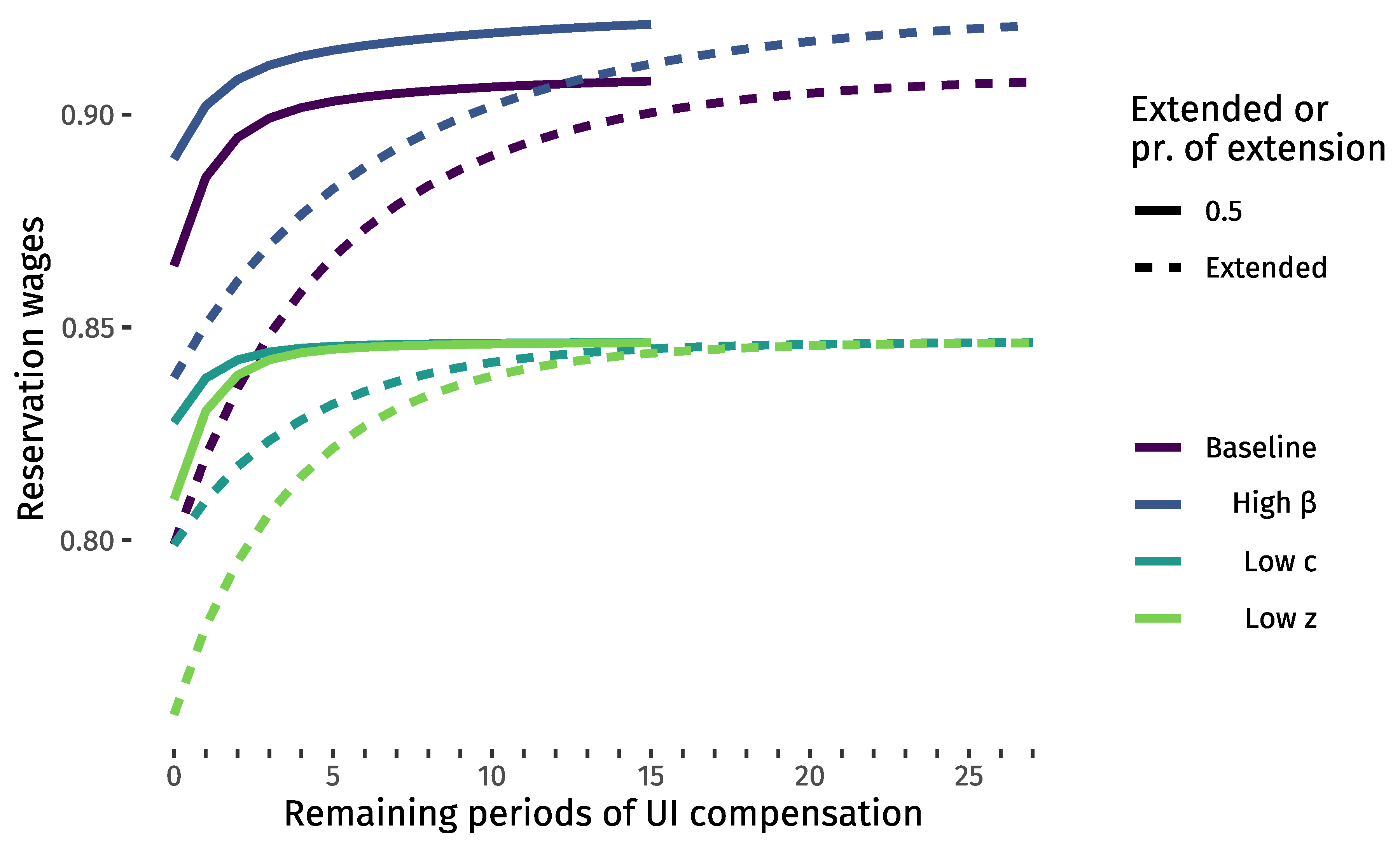
Appendix G. How β, c, and z Affect Reservation Wages

The main text shows how the probability of an extension and the extension’s length affect reservation wages. How a worker discounts the future and the value of nonwork affect a worker’s sequence of reservation wages. The effect is intuitive, as Figure A2 illustrates.
For a comparison, Figure A2 reports reservation wages for two cases shown in Figure 3 in purple. The solid purple line reports the sequence of reservation wages upon an extension and the broken purple line reports the sequence of reservation wages when the probability of extension is perceived to be 0.5. When β increases, workers are more patient. They are more selective throughout unemployment spells, and their sequences of reservation wages shift upward. The higher- β case is depicted in dark blue. When c is lower, workers receive less in UI compensation each period. They are less selective selective through unemployment spells, and their sequences of reservation wages shift downward. This is depicted in light blue. Because workers have the same β and the same z in the baseline and low-c parameterizations, the reservation wage upon an extension when there are no remaining periods of UI compensation are the same. In contrast, when z is lower, which is depicted in green, sequences of reservation wages are lower throughout workers’ unemployment spells.
Figure A2. How β , c, and z affect reservation wages. The baseline reports the values from Figure 3 in purple. Relative to the baseline, the effect of increasing the discount factor and lowering UI compensation are illustrated in blue and green. Solid lines correspond to instances when benefits have been extended. Broken lines correspond to instances where a worker believes the probability of extension is 0.5. Parameter changes affect the entire sequence of reservation wages.
Risks 11 00171 g0a2

Appendix H. Expressions When Wages Offers are Characterized by a Uniform Distribution

When job offers arrive from a uniform distribution, the optimal policy can be expressed in closed form. I start with the characterization of job search under expiring benefits when there is no chance of an extension.

Appendix H.1. Basic Job Search with Finite UI Benefits

As the proof of Proposition 1 in Appendix C suggests, the characterization starts with w R 0 . An implicit expression for w R 0 is given in Equation (A6). When wage offers are distributed uniformly over 0 , 1 , the expression for w R 0 can be developed as
w R 0 = z 1 β + β w ̲ w R 0 w R 0 d F w + w R 0 w ¯ w d F w = z 1 β + β w R 0 0 w R 0 d F w + w R 0 1 w d F w = z 1 β + β w R 0 F w R 0 + w 2 2 | w = w R 0 w = 1 = z 1 β + β w R 0 2 + 1 2 w R 0 2 2 .
Collecting terms yields a quadratic equation in terms of w R 0 :
0 = β 2 w R 0 2 w R 0 + z 1 β + β 2 .
The two roots of this expression are
w R 0 = 1 ± 1 4 β / 2 z 1 β + β / 2 β = 1 ± 1 β 1 + β 2 β z β ,
where the second equality uses the fact that
1 β 1 + β 2 β z = 1 β + 1 β β 2 β z = 1 β 2 2 β z + 2 β 2 z = 1 2 β z 1 β + β / 2 .
One of the roots yields a value for w R 0 that is above one and this root is not of economic interest. The root that is of economic interest is
w R 0 = 1 1 β 1 + β 2 β z β .
For β 0 , 1 , the reservation wages w R 0 will fall in the interior of the support of wage offers if 0 < z < 1 . The restriction on the flow value of nonwork follows from the requirement that 0 < w R 0 < 1 . The restriction that 0 < w R 0 requires
0 < 1 β 1 β 1 + β 2 β z 1 / 2 β 1 > 1 β 1 + β 2 β z 2 β z < 1 1 β 1 + β 1 β 1 β z > 1 2 β 1 β ,
which is guaranteed if z > 0 . The restriction that w R 0 < 1 requires
1 β 1 β 1 + β 2 β z 1 / 2 β < 1 1 β 1 + β 2 β z 1 / 2 > 1 β 1 + β 2 β z > 1 β 1 > z .
Expressions for w R n are arrived at recursively. Starting from (A4), for n = 1 , , N :
w R n = z + c 1 β + β w ̲ w R n 1 w R n 1 d F w + w R n 1 w ¯ w d F w = z + c 1 β + β w R n 1 0 w R n 1 d F w + w R n 1 1 w d F w = z + c 1 β + β w R n 1 2 + w 2 2 | w = w R n 1 w = 1 ,
which evaluates to
w R n = z + c 1 β + β 2 1 + w R n 1 2 .

Appendix H.2. Allowing for an Extension to Benefits

Reservation wages when the probability that benefits are extended with probability δ are implicitly given in (A12) and (A13). Using the same techniques as those in Appendix H.1, the expression for w R δ 0 can be developed as
w R δ 0 = z 1 β + β δ w ̲ w R Δ w R Δ d F w + w R Δ w ¯ w d F w + β 1 δ w ̲ w R δ 0 w R δ 0 d F w + w R δ 0 w ¯ w d F w = z 1 β + β δ 2 1 + w R Δ 2 + β 1 δ 2 1 + w R δ 0 2 .
The value w R Δ is known to the worker. Thus, w R δ 0 is the root to the quadratic equation
0 = β 1 δ 2 w R δ 0 2 w R δ 0 + z 1 β + β δ 2 1 + w R Δ 2 + β 1 δ 2 .
The economically relevant root is
w R δ 0 = 1 1 β 1 δ β + 2 z 1 β + β δ w R Δ 2 β 1 δ .
When δ = 0 , the expressions (A17) and (A19) agree.
As in Appendix H.1 above, expressions for w R δ n are arrived at recursively. Starting from (A11), for n 1 , , N :
w R δ n = z + c 1 β + β δ w ̲ w R n 1 + Δ w R n 1 + Δ d F w + w R n 1 + Δ w ¯ w d F w + β 1 δ w ̲ w R δ n 1 w R δ n 1 d F w + w R δ n 1 w ¯ w d F w .
Using the assumption about uniform wage offers, the latter evaluates to
w R δ n = z + c 1 β + β 2 1 + δ w R n 1 + Δ 2 + 1 δ w R δ n 1 2 .

Appendix H.3. Welfare

Computer code that conducts the numerical experiments makes use of expressions for expected welfare.
The value function for a worker entitled to n periods of UI compensation and wage offer w to accept or reject is
V w , n = max reject , accept U n 1 , W .
The value function can be written
V w , n = w R n 1 β = z + c + β V w , n 1 d F w if w w R n w 1 β if w w R n .
Expected welfare is
E V w , n = V w , n d F w .
If wages are uniformly distributed over 0 , 1 , then expected welfare evaluates to
E V w , n = 0 w R n w R n 1 β d F w + w R n 1 w 1 β d F w = w R n 2 1 β + 1 1 β w 2 2 | w = w R n 1 = w R n 2 1 β + 1 w R n 2 1 β 1 2 = 1 1 β 1 + w R n 2 2 .

Notes

1
Triggers for EB weeks may involve thresholds based on (1) a moving average of a state’s unemployment rate, or (2) the insured unemployment rate, which is the ratio of unemployment-compensation claimants divided by individuals in jobs covered by unemployment compensation (so, for example, not the self-employed and gig-economy workers) (Whittaker and Isaacs 2022). Chodorow-Reich and Coglianese (2019, p. 158, Figure 2) show data on the number UI recipients who claim regular, EB, and emergency weeks created by temporary extension. Extended benefits are relied upon less frequently than emergency benefits.
2
“When a state triggers off of an EB period, all EB benefit payments in the state cease immediately” (Whittaker and Isaacs 2022, p. 7).
3
The dates for this thought experiment come from data in (Rothstein 2011, p. 150, Table 1) and data available at https://oui.doleta.gov/unemploy/claims_arch.asp, accessed on 27 September 2023. Trigger dates for extended benefits and the EUC program are included in Supplementary Materials.
4
As of 11 August 2023, the 13 March date is reported on the Centers for Disease Control and Prevention’s COVID-19 timeline.
5
In addition, workers in 18 states faced a cutoff in compensation-benefit generosity when their states opted out of the FPUC and PUA progams in June 2021, before the programs were set to expire in September 2021, citing labor-supply issues (Holzer et al. 2021). There are many other parts to the UI system that are beyond the scope of this paper. Whittaker and Isaacs (2014, 2022) and Spadafora (2023) provide excellent, detailed coverage of the UI system. Fujita (2010), Rothstein (2011), and Chodorow-Reich and Coglianese (2019) provide excellent discussion of the many temporary programs.
6
In Krueger and Mueller’s (2016) survey on reservation wages, which I discuss below, over half of respondents with less than 3 months of unemployment duration report have no savings.
7
Ljungqvist and Sargent (2018) provide an informative textbook exposition. Rogerson et al. (2005) show how a similar decision-making environment fits into larger models of the macroeconomy that feature search.
8
Appendix C considers the case where the support of wages is w ̲ , . In that case, I establish that T contracts through direct verification, which requires more algebra.
9
Expression (11) is a generalization of Equation (6.3.3) in (Ljungqvist and Sargent 2018, p. 163). More details are provided in Appendix D.
10
Appendix E also shows that the support of wages can be extended to 0 , .
11
This assumption offers the opportunity to compare numerical work with closed-form expressions. Replication files for the paper compare reservation wages computed using closed-form expressions with those computed using Monte Carlo integration. Closed-form expressions are shared in Appendix H.
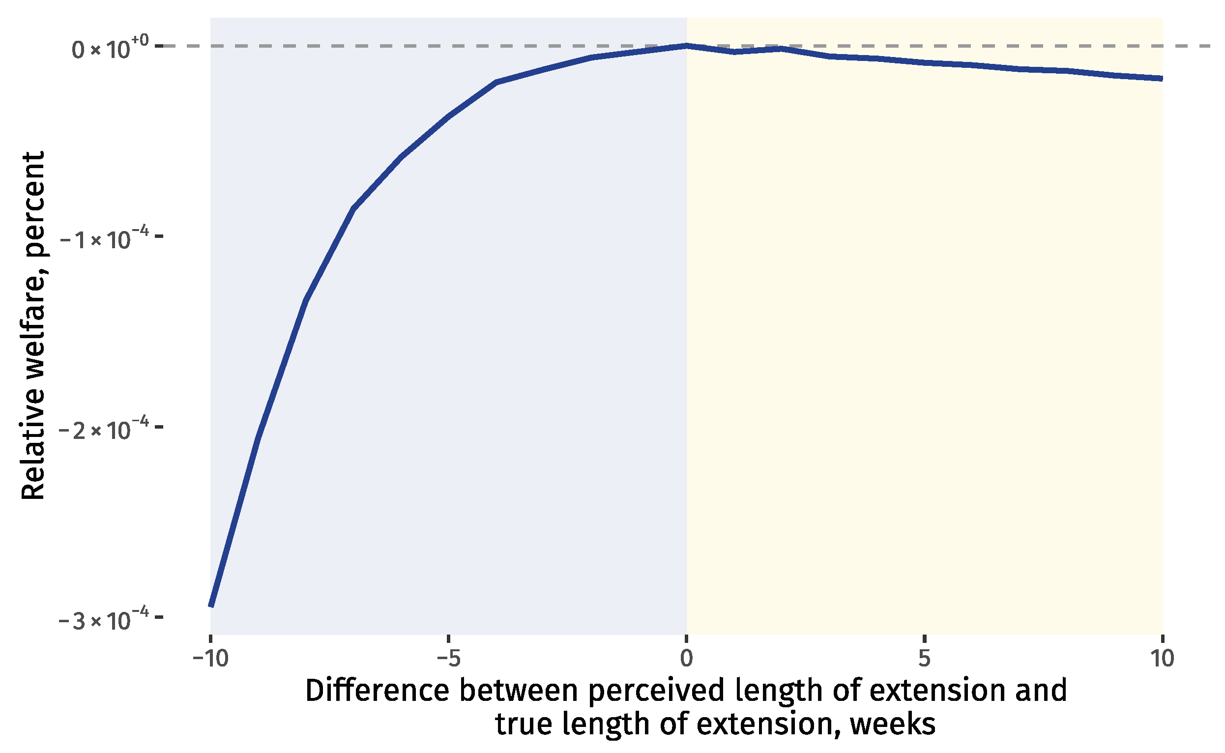
12
The simulations suggest that welfare is relatively flat, requiring a large number of runs.
13
Less is known about how psychology influences the job search. Two examples are provided by DellaVigna and Paserman (2005) and Paserman (2008), who study how impatience affects searching.
14
In related work, Shimer and Werning (2008) establish that optimal UI compensation involves constant or nearly constant benefits and, thus, a single reservation wage. Both papers informatively consider cases where workers save.
15
Autor and Duggan (2003) and Khemka et al. (2017) provide background.
16
Using the value function in this way is also achieved by Ross (1983).

References

  1. Acemoglu, Daron. 2001. Good jobs versus bad jobs. Journal of Labor Economics 19: 1–21. [Google Scholar] [CrossRef]
  2. Acemoglu, Daron. 2009. Introduction to Modern Economic Growth. Princeton: Princeton University Press. [Google Scholar]
  3. Akerlof, George A., and Janet L. Yellen. 1990. The fair wage-effort hypothesis and unemployment. The Quarterly Journal of Economics 105: 255. [Google Scholar] [CrossRef]
  4. Albert, Sarah, Olivia Lofton, Nicolas Petrosky-Nadeau, and Robert G. Valletta. 2022. Unemployment Insurance Withdrawal. FRBSF Economic Letter. 2022-09. Available online: https://www.frbsf.org/economic-research/publications/economic-letter/2022/april/unemployment-insurance-withdrawal/ (accessed on 27 September 2023).
  5. Anquandah, Jason S., and Leonid V. Bogachev. 2019. Optimal stopping and utility in a simple model of unemployment insurance. Risks 7: 94. [Google Scholar] [CrossRef]
  6. Autor, David H., and Mark G. Duggan. 2003. The rise in the disability rolls and the decline in unemployment. The Quarterly Journal of Economics 118: 157–206. [Google Scholar] [CrossRef]
  7. Barbanchon, Thomas Le, Roland Rathelot, and Alexandra Roulet. 2019. Unemployment insurance and reservation wages: Evidence from administrative data. Journal of Public Economics 171: 1–17. [Google Scholar] [CrossRef]
  8. Bewley, Truman F. 1999. Why Wages Don’t Fall During a Recession. Cambridge, MA: Harvard University Press. [Google Scholar]
  9. Boar, Corina, and Simon Mongey. 2020. Dynamic Trade-Offs and Labor Supply under the Cares Act. Working Paper 27727. Cambridge: National Bureau of Economic Research. [Google Scholar] [CrossRef]
  10. Boone, Christopher, Arindrajit Dube, Lucas Goodman, and Ethan Kaplan. 2021. Unemployment insurance generosity and aggregate employment. American Economic Journal: Economic Policy 13: 58–99. [Google Scholar] [CrossRef]
  11. Bryant, Victor. 1985. Metric Spaces. Cambridge: Cambridge University Press. [Google Scholar] [CrossRef]
  12. Burdett, Kenneth. 1979. Unemployment insurance payments as a search subsidy: A theoretical analysis. Economic Inquiry 17: 333–43. [Google Scholar] [CrossRef]
  13. Burdett, Kenneth, and Tara Vishwanath. 1988. Declining reservation wages and learning. The Review of Economic Studies 55: 655–65. [Google Scholar] [CrossRef]
  14. Caplin, Andrew, and John V. Leahy. 2019. Wishful Thinking. Working Paper 25707. Cambridge: National Bureau of Economic Research. [Google Scholar] [CrossRef]
  15. Card, David, and Phillip B. Levine. 2000. Extended benefits and the duration of UI spells: Evidence from the New Jersey extended benefit program. Journal of Public Economics 78: 107–38. [Google Scholar] [CrossRef]
  16. Card, David, Andrew Johnston, Pauline Leung, Alexandre Mas, and Zhuan Pei. 2015. The effect of unemployment benefits on the duration of unemployment insurance receipt: New evidence from a regression kink design in missouri, 2003–2013. American Economic Review 105: 126–30. [Google Scholar] [CrossRef]
  17. Card, David, Raj Chetty, and Andrea Weber. 2007. The spike at benefit exhaustion: Leaving the unemployment system or starting a new job? American Economic Review 97: 113–18. [Google Scholar] [CrossRef]
  18. Chetty, Raj. 2006. A general formula for the optimal level of social insurance. Journal of Public Economics 90: 1879–901. [Google Scholar] [CrossRef]
  19. Chetty, Raj. 2008. Moral hazard versus liquidity and optimal unemployment insurance. Journal of Political Economy 116: 173–234. [Google Scholar] [CrossRef]
  20. Chetty, Raj. 2009. Sufficient statistics for welfare analysis: A bridge between structural and reduced-form methods. Annual Review of Economics 1: 451–88. [Google Scholar] [CrossRef]
  21. Chetty, Raj, and Amy Finkelstein. 2013. Social insurance: Connecting theory to data. In Handbook of Public Economics. Amsterdam: Elsevier, vol. 5, pp. 111–93. [Google Scholar] [CrossRef]
  22. Chodorow-Reich, Gabriel, and John Coglianese. 2019. Recession Ready: Fiscal Policies to Stabilizethe American Economy. Chapter Unemployment Insurance and Macroeconomic Stabilization, The Hamilton Project and The Washington Center for Equitable Growth. Washington, DC: Brookings Institution, pp. 153–180. [Google Scholar]
  23. Chodorow-Reich, Gabriel, and Loukas Karabarbounis. 2016. The cyclicality of the opportunity cost of employment. Journal of Political Economy 124: 1563–618. [Google Scholar] [CrossRef]
  24. Chodorow-Reich, Gabriel, John Coglianese, and Loukas Karabarbounis. 2019. The macro effects of unemployment benefit extensions: A measurement error approach. The Quarterly Journal of Economics 134: 227–79. [Google Scholar] [CrossRef]
  25. DellaVigna, Stefano, and M. Daniele Paserman. 2005. Job search and impatience. Journal of Labor Economics 23: 527–88. [Google Scholar] [CrossRef]
  26. Dieterle, Steven, Otávio Bartalotti, and Quentin Brummet. 2020. Revisiting the effects of unemployment insurance extensions on unemployment: A measurement-error-corrected regression discontinuity approach. American Economic Journal: Economic Policy 12: 84–114. [Google Scholar] [CrossRef]
  27. Faberman, R. Jason, Andreas Mueller, and Ayşegül Şahin. 2022. Has the Willingness to Work Fallen during the Covid Pandemic? Labour Economics 79: 102275. [Google Scholar] [CrossRef]
  28. Farber, Henry S., and Robert G. Valletta. 2015. Do extended unemployment benefits lengthen unemployment spells?: Evidence from recent cycles in the u.s. labor market. Journal of Human Resources 50: 873–909. [Google Scholar] [CrossRef]
  29. Farber, Henry S., Jesse Rothstein, and Robert G. Valletta. 2015. The effect of extended unemployment insurance benefits: Evidence from the 2012–2013 phase-out. American Economic Review 105: 171–76. [Google Scholar] [CrossRef]
  30. Fujita, Shigeru. 2010. Economic Effects of the Unemployment Insurance Benefit. Business Review Q4. Available online: https://www.philadelphiafed.org/the-economy/macroeconomics/economic-effects-of-the-unemployment-insurance-benefit (accessed on 27 September 2023).
  31. Hagedorn, Marcus, Fatih Karahan, and Iourii Manovskii Kurt Mitman. 2019. Unemployment Benefits and Unemploymentin the Great Recession: The Role of Equilibrium Effects. Federal Reserve Bank of New York Staff Report No. 646. Available online: https://www.newyorkfed.org/research/staff_reports/sr646 (accessed on 27 September 2023).
  32. Hagedorn, Marcus, Iourii Manovskii, and Kurt Mitman. 2016. Interpreting Recent Quasi-Experimental Evidence on the Effects of Unemployment Benefit Extensions. Technical Report. Cambridge: National Bureau of Economic Research. [Google Scholar] [CrossRef]
  33. Hendren, Nathaniel. 2017. Knowledge of future job loss and implications for unemployment insurance. American Economic Review 107: 1778–823. [Google Scholar] [CrossRef]
  34. Holzer, Harry J., R. Glenn Hubbard, and Michael R. Strain. 2021. Did Pandemic Unemployment Benefits Reduce Employment? Evidence from Early State-Level Expirations in June 2021. Working Paper 29575. Cambridge: National Bureau of Economic Research. [Google Scholar] [CrossRef]
  35. Jäger, Simon, Benjamin Schoefer, Samuel Young, and Josef Zweimüller. 2020. Wages and the value of nonemployment. The Quarterly Journal of Economics 135: 1905–63. [Google Scholar] [CrossRef]
  36. Johnston, Andrew C., and Alexandre Mas. 2018. Potential unemployment insurance duration and labor supply: The individual and market-level response to a benefit cut. Journal of Political Economy 126: 2480–522. [Google Scholar] [CrossRef]
  37. Kahn, Lisa B. 2011. Unemployment insurance and job search in the great recession: Comments and discussion. Brookings Papers on Economic Activity 42: 205–10. [Google Scholar]
  38. Kekre, Rohan. 2023. Unemployment insurance in macroeconomic stabilization. Review of Economic Studies 90: 2439–80. [Google Scholar] [CrossRef]
  39. Khemka, Gaurav, Steven Roberts, and Timothy Higgins. 2017. The impact of changes to the unemployment rate on australian disability income insurance claim incidence. Risks 5: 17. [Google Scholar] [CrossRef]
  40. Kroft, Kory, and Matthew J. Notowidigdo. 2016. Should unemployment insurance vary with the unemployment rate? theory and evidence. The Review of Economic Studies 83: 1092–124. [Google Scholar] [CrossRef]
  41. Krueger, Alan B., and Andreas I. Mueller. 2016. A contribution to the empirics of reservation wages. American Economic Journal: Economic Policy 8: 142–79. [Google Scholar] [CrossRef]
  42. Krueger, Alan B., and Bruce D. Meyer. 2002. Labor supply effects of social insurance. In Handbook of Public Economics. Amsterdam: Elsevier, chp. 33. pp. 2327–92. [Google Scholar] [CrossRef]
  43. Lalive, Rafael. 2007. Unemployment benefits, unemployment duration, and post-unemployment jobs: A regression discontinuity approach. American Economic Review 97: 108–12. [Google Scholar] [CrossRef]
  44. Lalive, Rafael, and Josef Zweimüller. 2004. Benefit entitlement and unemployment duration. Journal of Public Economics 88: 2587–616. [Google Scholar] [CrossRef]
  45. Landais, Camille, and Johannes Spinnewijn. 2021. The value of unemployment insurance. The Review of Economic Studies 88: 3041–85. [Google Scholar] [CrossRef]
  46. Landais, Camille, Pascal Michaillat, and Emmanuel Saez. 2018. A macroeconomic approach to optimal unemployment insurance: Theory. American Economic Journal: Economic Policy 10: 152–81. [Google Scholar] [CrossRef]
  47. Ljungqvist, Lars, and Thomas J. Sargent. 2017. The fundamental surplus. American Economic Review 107: 2630–65. [Google Scholar] [CrossRef]
  48. Ljungqvist, Lars, and Thomas J. Sargent. 2018. Recursive Macroeconomic Theory, 4th ed. Cambridge, MA: The MIT Press. [Google Scholar]
  49. Marinescu, Ioana. 2017. The general equilibrium impacts of unemployment insurance: Evidence from a large online job board. Journal of Public Economics 150: 14–29. [Google Scholar] [CrossRef]
  50. Marinescu, Ioana, and Daphné Skandalis. 2021. Unemployment insurance and job search behavior. The Quarterly Journal of Economics 136: 887–931. [Google Scholar] [CrossRef]
  51. Marinescu, Ioana, Daphné Skandalis, and Daniel Zhao. 2021. The impact of the federal pandemic unemployment compensation on job search and vacancy creation. Journal of Public Economics 200: 104471. [Google Scholar] [CrossRef] [PubMed]
  52. McCall, J. J. 1970. Economics of information and job search. The Quarterly Journal of Economics 84: 113–26. [Google Scholar] [CrossRef]
  53. Mitman, Kurt, and Stanislav Rabinovich. 2015. Optimal unemployment insurance in an equilibrium business-cycle model. Journal of Monetary Economics 71: 99–118. [Google Scholar] [CrossRef]
  54. Mortensen, Dale T. 1977. Unemployment insurance and job search decisions. Industrial and Labor Relations Review 30: 505–17. [Google Scholar] [CrossRef]
  55. Nekoei, Arash, and Andrea Weber. 2017. Does extending unemployment benefits improve job quality? American Economic Review 107: 527–61. [Google Scholar] [CrossRef]
  56. Paserman, M. Daniele. 2008. Job search and hyperbolic discounting: Structural estimation and policy evaluation. The Economic Journal 118: 1418–52. [Google Scholar] [CrossRef]
  57. Petrosky-Nadeau, Nicolas. 2020. Reservation benefits: Assessing job acceptance impacts of increased UI payments. In Federal Reserve Bank of San Francisco, Working Paper Series. Cambridge: National Bureau of Economic Research. [Google Scholar] [CrossRef]
  58. Petrosky-Nadeau, Nicolas, and Robert G. Valletta. 2021. UI generosity and job acceptance: Effects of the 2020 CARES act. In Federal Reserve Bank of San Francisco, Working Paper Series. San Francisco: Federal Reserve Bank of San Francisco, Working Paper 2021-13. [Google Scholar] [CrossRef]
  59. Rogerson, Richard, Robert Shimer, and Randall Wright. 2005. Search-theoretic models of the labor market: A survey. Journal of Economic Literature 43: 959–88. [Google Scholar] [CrossRef]
  60. Ross, Sheldon. 1983. Introduction to Stochastic Dynamic Programming. New York: Academic Press. [Google Scholar] [CrossRef]
  61. Rothstein, Jesse. 2011. Unemployment insurance and job search in the great recession. Brookings Papers on Economic Activity 42: 143–96. [Google Scholar] [CrossRef]
  62. Rutledge, Matthew S. 2011. The Impact of Unemployment Insurance Extensions on Disability Insurance Application and Allowance Rates. Boston College Center for Retirement Research Working Paper No. 2011-17. Available online: https://doi.org/10.2139/ssrn.1956008 (accessed on 27 September 2023).
  63. Schmieder, Johannes F., and Till von Wachter. 2016. The effects of unemployment insurance benefits: New evidence and interpretation. Annual Review of Economics 8: 547–81. [Google Scholar] [CrossRef]
  64. Shimer, Robert, and Iván Werning. 2007. Reservation wages and unemployment insurance. The Quarterly Journal of Economics 122: 1145–85. [Google Scholar] [CrossRef]
  65. Shimer, Robert, and Iván Werning. 2008. Liquidity and insurance for the unemployed. American Economic Review 98: 1922–42. [Google Scholar] [CrossRef]
  66. Solon, Gary. 1979. Labor supply effects of extended unemployment benefits. The Journal of Human Resources 14: 247. [Google Scholar] [CrossRef]
  67. Spadafora, Francesco. 2023. U.S. unemployment insurance through the covid-19 crisis. Journal of Government and Economics 9: 100069. [Google Scholar] [CrossRef]
  68. Whittaker, Julie M., and Katelin P. Isaacs. 2014. Extending Unemployment Compensation Benefits during Recessions. Technical Report, Congressional Research Service Report RL34340. Washington, DC: Congressional Research Service. [Google Scholar]
  69. Whittaker, Julie M., and Katelin P. Isaacs. 2022. Unemployment Insurance (UI) Benefits: Permanent-Law Programs and the COVID-19 Pandemic Response. Technical Report, Congressional Research Service Report R46687. Washington, DC: Congressional Research Service. [Google Scholar]
  70. Yellen, Janet L. 1984. Efficiency wage models of unemployment. The American Economic Review 74: 200–5. [Google Scholar]
Figure 1. Index of Google searches for “unemployment benefits extension”. These data represent relative search frequency from the week containing 5 January 2020 to the week containing 27 February 2022. The series is normalized so that the highest-intensity week is set to 100. Source: Google Trends.
Risks 11 00171 g001
Figure 2. Evolution of remaining periods of UI benefits. The worker believes benefits will be extended with probability δ and the extension will add Δ periods they are allowed to claim UI compensation benefits.
Risks 11 00171 g002
Figure 3. Sequences of reservation wages. The dark blue line depicts the sequence of reservation wages once an extension has occurred. These reservation wages lie below the sequences of reservation wages when there is a chance of extension, meaning the worker is less selective when there is no chance of extension. Sequences were generated using F w = w , c = 0.42 , z = 0.42 , N = 15 , Δ = 13 , β = 0.95 , and δ 0.1 , 0.5 , 0.9 .
Risks 11 00171 g003
Figure 4. Welfare loss when a worker misperceives the likelihood of extension. The horizontal axis is the subjective belief a worker holds when computing the sequence of reservation wages less the true probability that benefits are extended. The blue line depicts the loss in welfare associated with misperceiving the probability that benefits are extended. When the worker’s subjective beliefs line up with the true probability at 0 along the horizontal axis, then the welfare loss is zero. The shaded blue region denotes cases where a worker is too pessimistic about an extension. The shaded yellow region denotes cases where a worker is too optimistic about an extension. The true probability of an extension is 0.5.
Risks 11 00171 g004
Figure 5. Welfare loss when a worker misperceives the length of extension. The horizontal axis is the subjective belief about the length of an extension a worker holds when computing the sequence of reservation wages less the true length of an extension. The blue line depicts the loss in welfare. When the worker’s subjective beliefs line up with the true length of an extension at 0 along the horizontal axis, then the welfare loss is zero. The region shaded blue denotes cases where a worker is too pessimistic about the length of the extension. The region shaded yellow denotes cases where a worker is too optimistic about the length of the extension. The true length of an extension is 25.
Risks 11 00171 g005
Figure 6. Simulated statistics for a worker’s choices about job offers when the worker misperceives the true chance of an extension. The horizontal axis reports the subjective belief a worker holds about the chance of an extension when computing the sequence of reservation wages less the true probability that benefits are extended. The unit of measurement along the horizontal axis is probability. The shaded regions highlight cases where a worker believes an extension is unlikely. The top panel shows the average number of periods a worker spends unemployed relative to the number of periods that would be spent in unemployment if the true probability of an extension were known. The bottom panel shows the average accepted wage, reported as the percent away from the optimal wage.
Risks 11 00171 g006
Figure 7. Simulated statistics for a worker’s choices about job offers when the worker misperceives the length of an extension. The horizontal axis reports the subjective belief a worker holds about the length of an extension when computing the sequence of reservation wages less the true extension length. The unit of measurement along the horizontal axis is periods or weeks. The shaded regions highlight cases where a worker believes an extension will be shorter than what occurs. The top panel shows the average number of periods a worker spends unemployed relative to the number of periods that would be spent in unemployment if the true length of extension were known. The bottom panel shows the average accepted wage, reported as the percent away from the optimal wage.
Risks 11 00171 g007
Disclaimer/Publisher’s Note: The statements, opinions and data contained in all publications are solely those of the individual author(s) and contributor(s) and not of MDPI and/or the editor(s). MDPI and/or the editor(s) disclaim responsibility for any injury to people or property resulting from any ideas, methods, instructions or products referred to in the content.

