Abstract
Log-concavity and log-convexity play a key role in various scientific fields, especially in those where the distinction between exponential and non-exponential distributions is necessary for inferential purposes. In the present study, we introduce a testing procedure for the tail part of a distribution which can be used for the distinction between exponential and non-exponential distributions. The conspiracy and catastrophe principles are initially used to establish a characterization of (the tail part of) the exponential distribution, which is one of the main contributions of the present work, leading the way for the construction of the new test of fit. The proposed test and its implementation are thoroughly discussed, and an extended simulation study has been undertaken to clarify issues related to its implementation and explore the extent of its capabilities. A real data case is also investigated.
1. Introduction
In Statistics, the problem of determining the underlying mechanism, i.e., the model governing the data, is a classical statistical problem. Some of the most popular continuous distributions in biomedicine, survival and reliability analysis, actuarial science and risk management and in engineering and technical systems are among others, the exponential, the lognormal, the Gamma, the inverse Gaussian, the Weibull and the Pareto distributions. Indeed, for instance, the inverse Gaussian distribution is frequently encountered in fields such as medicine (e.g., cardiology), environmental sciences (e.g., hydrology) or humanities (e.g., linguistics) (Chhikara and Folks 1977). On the other hand, distributions like the Weibull, the Gamma or the Pareto are applicable among others, in insurance, survival modeling and lifetime problems (see for instance Huber-Carol and Vonta 2004; Tremblay 1992). Observe that each of these distributions is frequently referred to as light- or heavy-tailed distribution according to whether the tail part is lighter or heavier than that of the exponential distribution (see e.g., Bryson 1974).
The catastrophe and conspiracy principles provide the fundamental distinction between phenomena characterized by distributions with tails heavier and those with tails lighter than the exponential distribution. Extreme and rare events stemming from these principles can be found in areas such as economics, insurance science, queuing theory and reliability, and in practice, they are represented as large insurance claims, long queues, strong earthquakes and hurricanes, heavy rains, or critical components in structural reliability that fail due to extremely large values, etc. Although the cause of occurrence of such rather exceptional rare events is associated with the tail part of the probability distribution, the mechanisms underlying such occurrences are fundamentally different.
According to the catastrophe principle (or single big jump, Foss et al. (2007)), which in general refers to more that two () heavy-tailed random variables, rare events occur most likely due to the smallest possible number of contributing components. Indeed, let us denote by , , a random sample of heavy-tailed variables, the summation of which is assumed to be large. Then, it is most likely that this is due to one of these variables being large and all others being typical. If one considers the claims received by an insurance company, it is straightforward to realize that the financial instability may occur as a result of just one extremely high claim. In fact, the class of heavy-tailed distributions and all its subclasses, like the subexponential class of distributions, assists in understanding the occurrence of such outliers or rather the occurrence of extremely large outliers which occur for a single extreme value, which is so large that all other values appear to be negligible in comparison.
As opposed to the class of heavy-tailed distributions, light-tailed ones tend to obey the so-called conspiracy principle, according to which rare events most likely occur as a result of a combination of a large number of equally contributing components. A classical example for the above principle materializes in the context of queues, where rare events such as large delays or backlogs occur as a result of a “conspiracy” which involves a large number of customers or jobs, all arriving at the same moment.
It should be noted that light-tailed distributions are associated with log-concavity while heavy-tailed ones are associated with log-convexity (Asmussen and Lehtomaa 2017). It is vital for instance in actuarial science, geosciences, survival analysis or reliability settings to distinguish between an exponential distribution, a light-tailed or a heavy tailed one when the researcher is interested in the tail part of the distribution or more generally, the part of the distribution exceeding a certain threshold. Thus, such settings are of great importance due to their practical implications, making the investigation and the modeling of the tail part of such distributions an important problem with practical implications.
In this work, we present and investigate a test of fit by focusing on the tail part of a distribution, i.e., by relying exclusively on the extreme portion of the available data. The fact that the specific small portion of data is sufficient for testing purposes is due to the fact that this part of the data is associated with a tail characterization that distinguishes exponential and non-exponential distributions. As opposed to classical tests (see e.g., Baratpour and Rad 2012; Huber-Carol et al. 2002; Jimenez-Gamero and Batsidis 2017; Novikov et al. 2015; Rogozhnikov and Lemeshko 2012; Vonta et al. 2012), in this work, the emphasis is placed exclusively on the tail by ignoring the rest of the distribution. It should be noted that although classical tests based on the entire dataset often fail to reject a null hypothesis, the proposed testing procedure checks the fit of the tail and makes a decision exclusively on the available data from the extreme part of the distribution. At the same time, it should be also noted that the proposed test does not provide any indication on the heaviness (or lightness) of the tail part of the distribution, as is often completed through the class of tail index tests (as e.g., in Jureckova and Picek 2001; Kim and Lee 2016). In that sense, the proposed test can be considered as a goodness of fit test for exponentiality via the use of the extreme region of data. Note that the proposed tail test is triggered by the catastrophe and conspiracy principles to be used for distinguishing between exponential and non-exponential distributions, i.e., light or heavy-tailed distributions when the interest lies on the part of the dataset exceeding a certain threshold. At the same time, this paper contributes to the relevant literature by paving the way to verify the properties of log-concavity and log-convexity. The importance of the proposed technique has significant practical implications. Indeed, the motivation behind the proposed test is the assessment of risk from high damages, large claims, economic collapses, etc., all of which are associated with the right tail of the distribution being of interest. Some preliminary results have been presented in Karagrigoriou et al. (2022) and Papasotiriou (2021). The details of the formulation of the test statistic are provided in Section 2. The proposed test statistic with extended simulations which clarify issues related to the implementation of the test is given in Section 3. A real case application on fire insurance data is presented and analyzed in Section 4, and some concluding remarks are provided in Section 5.
2. Log-Concavity, Log-Convexity and the Subexponential Class of Distributions
In this section, we present the details connecting log-concavity and log-convexity to light and heavy-tailed distributions and discuss the subexponential class of distributions. Furthermore, a special random variable for distinguishing between exponential, heavy and light-tailed distributions will be defined, and its properties will be presented and discussed. This variable will be later used for presenting a test for the tail part of the distribution.
2.1. Log-Concavity and Log-Convexity
For heavy-tailed distributions, the tail part is asymptotically heavier than the tail of the exponential distribution. In other words, one could state that the tail part of the distribution decays to zero at a rate slower than that of the exponential distribution, which further implies that in such phenomena, extremely large values materialize with non-negligible probabilities.
On the other hand a light-tailed distribution has the “opposite” property of a heavy-tailed one, i.e., the tail part of the distribution is asymptotically bounded by that of an exponential distribution, and thus, it decays to zero at most as fast as the exponential distribution, i.e., for some threshold d.
A random variable is considered to be log-concave (log-convex) if the logarithm of its probability density function (pdf) is concave (convex). Both classes are substantially broad with appealing properties. It was recently demonstrated that light-tailed asymptotic behavior is associated with log-concave densities, while log-convexity seems to be connected to heavy-tailed behavior (Asmussen and Lehtomaa 2017). Indeed, a pdf of a log-concave variable is necessarily light-tailed, while the pdf is log-convex in the tail in classical heavy-tailed distributions like a regular varied distribution (RV), a lognormal distribution, or a Gamma distribution with a shape parameter less than 1. Note that the log-concavity of a density in a survival or reliability setting implies monotonically increasing hazard (and reversed hazard) rates (Gupta and Balakrishnan 2012), which further implies a sub-additive logarithm of the survivor function which, in turn, is equivalent to the property of new-is-better-than-used (NBU).
2.2. Subexponential Class of Distributions
The class of heavy-tailed distributions is quite broad consisting of various special subclasses which satisfy special extra regularity conditions. The focus in this work is on a very popular and important subclass, the subexponential class, which for two independent random variables and is defined by
for any threshold d. The above definition is closely related to the so-called catastrophe principle, also known as the single jump principal, according to which the summation of and is large most likely if one of the X values involved is large, whereas the other remains typical. This subclass includes most of the common heavy-tailed parametric families like Pareto, negative exponential, Gamma and Weibull with a shape parameter , the beta distribution with both parameters being smaller than 1 and the F distribution with the degrees of freedom of the numerator being smaller than the degrees of freedom of the denominator. It should be pointed out that the Weibull and Pareto distributions are related to the theory of extremes (Fisher and Tippett 1928; Gnedenko 1943; Bagdonavičius et al. 2013). The Weibull distribution is used in industrial engineering to represent manufacturing and delivery times, in weather forecasting to describe the distribution of wind speed and in wireless communications for the modeling of fading channels. Many more applications can be found in reliability and industrial engineering, survival analysis, hydrology, etc. The special case of the Rayleigh distribution is often used to describe measurement data in the field of communications engineering and in the life testing of electrovacuum devices. On the other hand, as one should expect, the class of light-tailed distributions includes, among others, the Gamma and the Weibull with a shape parameter and the beta with both parameters larger than or equal to 1.
2.3. The Background for the Proposed Test
Given two independent random variables and , the preceding discussion stemming from (1) motivates the use of the following quantity as a way to distinguish between the heavy and the light-tailed case:
Indeed, R will be close to 1 for heavy-tailed variables since only one of them will be dominant and close to 0 for light-tailed variables due to their equal contribution. In fact, as shown by Lehtomaa (2015), the above observation holds true in great generality. Specifically, the conditional random variable
provides a sharp borderline between log-convexity and log-concavity, the values of which are expected to lie in the region for any threshold d. Thus, the function
can be considered as a generalization of the above with a similar interpretation: being close to 0 if the two variables contribute equally to the summation and being close to 1 if one of the variables is of the same magnitude as the summation for large d values. It is easy to observe that values of in the center of the interval are associated with exponentially distributed random variables, whereas log-concave (log-convex) distributed variables are associated with values in the lower (upper) half of the interval. Asmussen and Lehtomaa (2017) proved that for distributions that become eventually log-concave, we have the following:
while for distributions that become eventually log-convex, we have
At the same time, it is observed that for exponentially distributed variables and for any positive threshold d,
The latter result holds for any threshold (even for the entire data set) due to the fact that the conditional random variable is symmetric under exponentiality, which is a property that ceases to hold for non-exponential distributions having a lighter or heavier tail. In fact, for non-exponential distributions, the smaller the tail part (i.e., the larger the threshold), the sharper the limit in (5) and (6). It is important to point out that the distinction between exponential and non-exponential distributions having a lighter or heavier tail is required to be established on the tail part, since a distribution becomes eventually (i.e., as ) log-concave or log-convex as compared to the exponential distribution.
The results in Equations (5)–(7) clearly show that as we go away from the exponential distribution to heavier or lighter distributions, in (4) moves away from on either side of the real line (to the left for light and to the right for heavy-tailed distributions) with the only distribution on this class with being the exponential for all values of d. This characterization in terms of (5)–(7) will be used for setting up testing procedures for
- Exponential Distribution versus Heavy-Tailed Distribution:
- Exponential Distribution versus Light-Tailed Distribution:
Asmussen and Lehtomaa (2017) used the empirical counterpart of (4) for a graphical analysis. In this work, we are fully analyzing the behavior of the empirical counterpart of (4), to be presented in the following section, and to be used for testing (8) and (9). It is important to emphasize that the test is based on , i.e., a quantity that eventually characterizes the tail part of a distribution, and thus, it is based exclusively on data exceeding a threshold that tends to infinity.
3. The Proposed Test of Fit
3.1. The Test Statistic
The characterization discussed in the previous section will be used in this section as the vehicle for constructing a test of fit for testing (8) and (9) with the test statistic being the empirical counterpart of (4) given by
where is the indicator of A and
where and are random samples from two independent random variables belonging to the class given in (1), and d is a threshold usually representing a percentile of the associated distribution under the null hypothesis in (8) and (9), i.e., under exponentiality.
For illustrative purposes, Figure 1, Figure 2 and Figure 3 based on 25,000 simulations provide the empirical density of for the exponential distribution and for representative examples of a light-tailed distribution (Weibull with shape ) and a heavy-tailed distribution (Weibull with shape ) for samples of size and for different values of d. Observe that all figures provide the density for the entire data set (using as a threshold the 0th percentile—) accompanied by the densities for the portion of the data set above the 50th, 70th, 80th, 90th and 95th percentiles (Q50, Q70, Q80, Q90 and Q95). The same behavior is observed for small () as well as for large sample sizes () (results not shown). For the exponential distribution, observe that the general shape of the density of is not affected by the value of d and is in fact symmetric and centered at , which confirms that (7) holds true for any value of d. At the same time, the variability varies for different sample sizes, being larger than the one depicted in Figure 1 for small sample sizes () and smaller for larger sample sizes ().
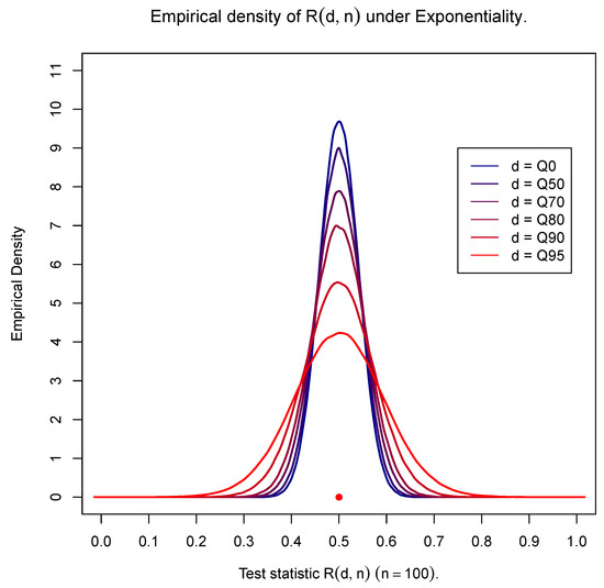
Figure 1.
Exponential distribution.
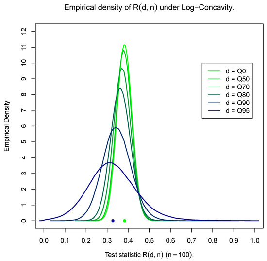
Figure 2.
Light-tailed distributions—Weibull (shape ).
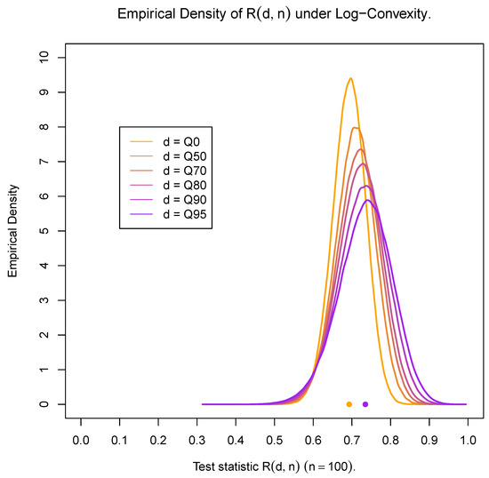
Figure 3.
Heavy-tailed distributions—Weibull (shape ).
On the other hand, Figure 2 and Figure 3 fully confirm expressions (5) and (6). Indeed, it is observed that as d increases (and the number of available data decreases), the limiting result in (5) is evident. One additional observation for the heavy-tailed case is the smaller variability as compared with the one observed for the light-tailed case as d increases. At the same time, as the threshold d tends to zero (including the case of the full data set), the distinction between the exponentiality and light- or heavy-tailed distributions becomes difficult. This is the reason classical tests, i.e., tests based on the entire data sets, are not always able to distinguish between exponential and non-exponential distributions. The test to be proposed below is resolving this matter by providing a tail test which manages to make the distinction and identify correctly the underlying distribution by examining solely the tail part over the threshold d.
As expected, the results are even more extreme as we move further away from the exponential distribution on either side of the particular value of the shape parameter of the distribution (being taken equal to in the above case).
Finally, note that the parameter values used in Figure 1, Figure 2 and Figure 3 do not affect the position of the associated distribution due to the invariance property of the scale parameter satisfied by all distributions considered in this and the subsequent sections. Also note that the position of the distribution of the test statistic in the exponential case in Figure 1 is the same irrespectively of the value of the shape parameter (here, it is taken to be equal to 1).
3.2. The Pairing and the Choice of Threshold
Based on the definition of the test statistic in (10) and the preceding discussion, we have to take under consideration two issues: namely, the sample pairing and the choice of the threshold d. Indeed, the test statistic in (10) requires two independent r.v. values, i.e., i.i.d. sample pairs and a threshold d that should be large enough due to the asymptotic nature of (5) and (6) but not too large, since a sufficient number of pairs should be available to ensure the reliable performance of the test. These two issues are addressed and dealt with in this subsection.
3.2.1. The Pairing
Observe that (10) requires as input a two-dimensional sequence of random variables. In case of a single random sample , without loss of generality, one could create two sequences by choosing any random pairing of the observations involved, as is the case when constructing the figures in the previous subsection. In the simplest case and for an even sample size n, one could take and , and thus create the two random samples required by the relevant theory. Although the original single sample is random and any random pairing will produce two random (sub)samples, one may question the pairing chosen. Any concern associated with the pairing could be resolved by choosing a fixed number of permutations. Indeed, before pairing, a number of permutations (i.e., random re-orderings) could help in overcoming concerns and diminish the influence of an extreme (outlier) value of the test statistic based on a single pairing chosen either randomly or intentionally or even the influence of a kind of dependence, sequential or otherwise. Then, the statistic given in (10) could be calculated as many times as the number of permutations, and then, the test statistic is set equal to the mean value of all repetitions. Figure 4, Figure 5 and Figure 6 attempt to shed some light into the issue of pairing with the use of a number of random pairings of independent samples from various distributions. All three figures reveal the consequences of pairing by providing the upper and lower limits and thus the extent of the range of the test statistic values for different permutations. Thus, the analysis shows a possibly downgraded (in relation to a real case scenario where independence may not be present) effect of pairing and the importance of choosing the mean value (or alternatively the median) of all test statistic values over all permutations. Note that for a two-sample problem, permutations may not be necessary, but they are still recommended to diminish the possibility of dependence between the observations of the two data sets.
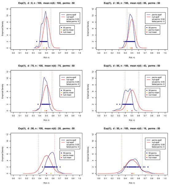
Figure 4.
Exponential distribution.
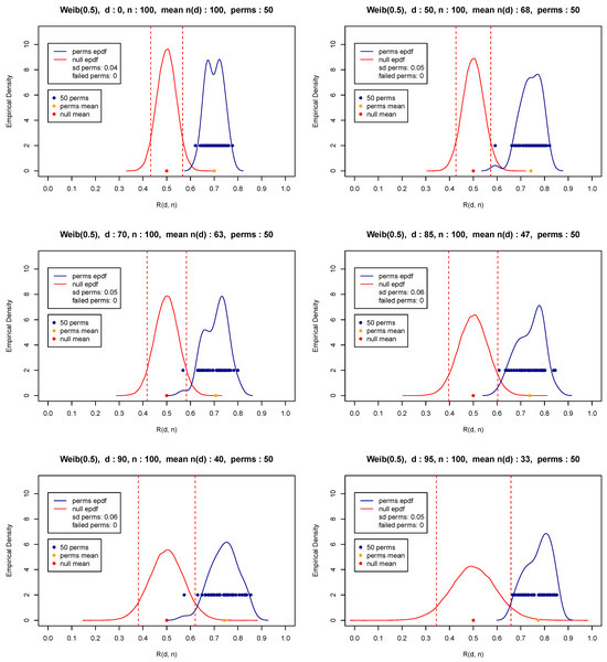
Figure 5.
Heavy-tailed distribution—Weibull, shape .
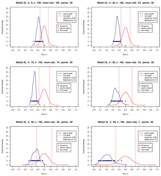
Figure 6.
Light-tailed distribution—Weibull, shape .
In what follows, we have chosen to perform 50 permutations, which is a number that appears to be more than satisfactory for practical purposes. In fact, our extended simulations show that any number of permutations at least equal to 50 gives a distribution with sufficient speed (insignificant computational cost) and a very small variability. At the same time, the execution of at least some permutations is highly recommended so that a balance or compromise is materialized to overcome possible sequential dependencies and diminish influential pairings. Figure 4, Figure 5 and Figure 6 present the distribution of for various thresholds based on 50 permutations (blue points and blue curve) of random samples of size from the exponential distribution with parameter values equal to 1 (Figure 4) and representative light and heavy-tailed distributions (Weibull with shape and 0.5—Figure 5 and Figure 6). The figures also show the mean (orange bullet) and the standard deviation of the 50 repetitions (denoted by sd perms) of the test statistic as well as the mean (red bullet) and the empirical pdf of the test statistic (red curve) under the null hypothesis in (8) and (9). Observe that these results reconfirm the theoretical results appearing in (5)–(7).
- Remarks:
- (1)
- For an odd sample size n, the smallest observation in the sample is removed, as it contributes the least amount of information to the test statistic as d increases.
- (2)
- For extremely large values of d, a larger number of permutations should be considered to ensure that sufficient number of observations and pairs will be available for the evaluation of the test statistic.
- (3)
- Note that although independence is a required assumption, the proposed pairing technique may be used even when a kind of dependence (even a weak one) is present. Although in such a case, the assumptions required for implementing the proposed methodology are not satisfied, the use of permutations is expected to minimize the effect of the particular type of dependence. As it turns out, the implementation of the proposed methodology on sequential or in general, dependent data, raises an issue that needs to be explored: namely, to thoroughly investigate whether the assumption of independence could be entirely dropped. This appears to be an important problem by itself not only from the theoretical point of view but also due to great practical implications, which we intend to investigate as part of an upcoming project.
3.2.2. The Threshold
Another vital issue is the selection of the threshold d in (10), which will satisfactorily distinguish between exponential, light and heavy-tailed distributions in terms of (5)–(7). Observe in Figure 4, Figure 5 and Figure 6 that as the threshold moves from (upper left corner) to (lower right corner), indicating the corresponding percentile of the associated distribution, the available number of observations , i.e., the number of observations having their matched paired summation larger than d, decreases. Indeed, observe for instance that for the light-tailed distribution with in Figure 6, is equal to 7, which is very small compared to exponential or heavy-tailed distributions being equal to 16 and 33, respectively (see Figure 4 and Figure 5).
As expected, small values of force several permutations to fail to contribute to the test statistic, resulting in less reliable and less accurate inferences, especially for extremely large values of d. It is reminded that the asymptotic nature in (5) and (6) refers to r.v values having eventually (i.e., as ) heavy or light-tailed distributions. As a result, it is quite natural that as the sample size increases, the threshold d chosen should represent an extremely high percentile for catching the asymptotic behavior of the tail part implied by those theoretical results.
3.2.3. The Test Statistic Evaluation
The behavior of , and the number of failed permutations based on 50 permutations have been fully explored for thresholds ranging from (the entire data set) to for distributions with various light as well as heavy-tailed parts.
Figure 7, Figure 8 and Figure 9 show representative results based on the Weibull distribution with shape values ranging from 0.1 (for a representative heavy-tailed distribution) to 1 (for the exponential distribution) and up to 1.9 (for a representative light-tailed distribution). Observe that the values remain in the vicinity of 0.5 (top-part of Figure 7) for the exponential distribution irrespectively of the value of the threshold d. On the other hand, the test statistic stays away from and more specifically over (toward 1) for heavy-tailed distributions (see the top part of Figure 8) and under (toward 0) for light-tailed distributions (see top part of Figure 9).
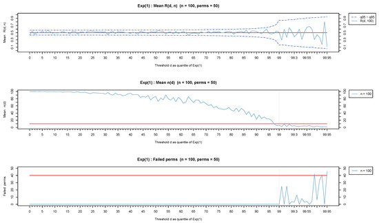
Figure 7.
Exponential distribution.
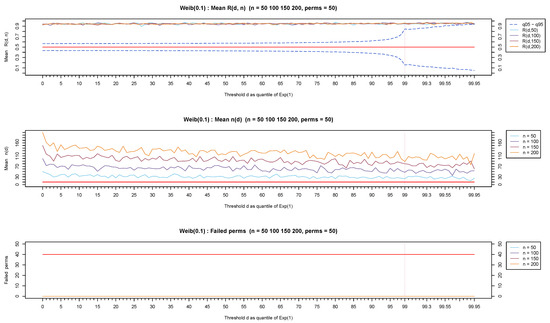
Figure 8.
Heavy-tailed distribution—Weibull, shape .
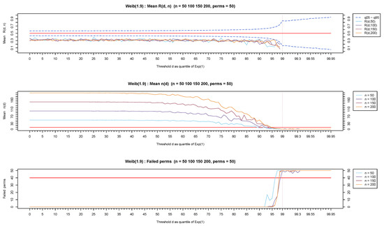
Figure 9.
Light-tailed distribution—Weibull, shape .
Observe that in all three cases but mostly for light-tailed distributions, the test statistic exhibits a fluctuation for large values of d which is due to a small number of available observations. The values for each threshold d are provided in the middle part of each figure, showing clearly that for any distribution but mostly for light-tailed ones, as the sample size decreases (from to ), there are veryfew observations left for the analysis. Extensive simulations have shown that (represented by a red horizontal line in the middle part of Figure 7, Figure 8 and Figure 9) is a reasonable minimum number of observations for reliable inferences. Observe that stays over the red horizontal line for all d values for heavy-tailed distributions (middle part of Figure 8) but crosses the red horizontal line for depending on n for light-tailed distributions (middle part of Figure 9) as well as for the exponential case but for a higher threshold (middle part of Figure 7).
We finally notice (lower part of Figure 7, Figure 8 and Figure 9) that mostly for light-tailed distributions, several permutations fail to contribute toward the test statistic when is small. Indeed, observe the lower part of Figure 9 where at least 40 permutations (represented by the red horizontal line in the lower part of Figure 9) fail to produce a value for when . Similar issues rarely appear in exponential or heavy-tailed distributions (low part of Figure 7 and Figure 8).
Based on all the above, we proceed to the recommendations given in Table 1 for proper thresholds d separately for light and heavy-tailed distributions and various sample sizes ( to ), which ensure simultaneously that the number at the specific threshold and the associated number of available permutations for calculating the test statistic are at least equal to 10, which appears to be a satisfactory choice for all practical purposes.

Table 1.
Recommended thresholds based on sample size.
3.3. Implementation of the Test Statistic
Based on the discussion in the previous sections, the test statistic for the testing problems in (8) and (9) is defined as the average of the empirical counterpart of given in (10), over B permutations executed, with the recommended number of permutations being equal to , namely:
where and is the indicator of A. According to the above discussion, the algorithmic procedure for the proposed tail test is as follows:
Algorithmic Procedure for the Evaluation of the Test Statistic
- 1.
- For a data set with an even number of observations , set and , (for n = odd, remove first the smallest observation).
- 2.
- Produce B random reorderings (permutations) of the data set and repeat Step 1 for each permutation.
- 3.
- Identify the proper threshold d by choosing the value of d corresponding to the sample size in Table 1, which is closer to n.
- 4.
- Evaluate for each of B permutations in Step 2 and for d obtained in Step 3, and calculate the value of in (12).
One of the most important facts for the proposed test statistic is that under the null hypothesis of exponentiality in (8) and (9), it is extremely stable in terms of the mean, while the variability is quite satisfactory, allowing for an easy way to handle critical points for testing purposes. Table 2, based on 25,000 simulations, provides for the series of thresholds and sample sizes of Table 1 the empirical values of the standard deviation of the test statistic in (12) under the null hypothesis. It is worth pointing out that the mean remains stable and equal to 0.50 for any sample size n and any threshold d (results not shown).
Table 2.
Recommended thresholds based on sample sizes and the corresponding standard deviations of the test statistic.
It is easily concluded that under the null hypothesis of exponentiality, the standardized test statistic follows a standard normal distribution, making its implementation straightforward. Observe that the normality under the null hypothesis comes naturally as a result of the discussion in Section 3.1 and Figure 1, where the distribution of the unstandardized test statistic is depicted. Additional visual verification is provided by Figure 10, which based on 15,000 simulations presents the behavior of the empirical distribution of the standardized test statistic for and four (4) extreme percentiles used for the threshold, namely and . The result is presented below:
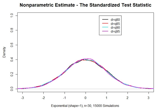
Figure 10.
Standardized test statistic, exponential distribution, n = 30—various thresholds.
Theorem 1.
Proof.
For fixed d, define so that
where the values are i.i.d. random variables with finite mean and finite variance, while the values are independent random variables which are not independent of , so that
where values are i.i.d.. Observe that
since, under the null hypothesis of exponentiality,
Observe also that , which in turn implies that
Then, it is easy to see utilizing Slutzky’s theorem that the following central limit theorem holds and in particular, we have as , that
where represents convergence in distribution. □
- Remarks:
- (1)
- We should point out that if , we have the classical central limit theorem with .
- (2)
- For the given in (12), we consider random re-orderings, i.e., bootstrap samples of size n without replacement, and apply Theorem 1 to the average of the B values of obtained, say , namely (see for instance Csorgo and Nasari 2013 and Rosalsky and Li 2017).
3.4. Performance of the Test—Size
In this and the subsequent section, we explore the capabilities of the proposed test in terms of the size and the power of the test against log-concave and log-convex distributions using for comparative purposes classical tests like the Kolmogorov–Smirnov (KS), Gnedenko (GN), Gini (GI) and the Shapiro–Wilk (SW) (see e.g., Shapiro and Wilk (1972); Gail and Gastwirth (1978); Ascher (1990)). Details about these competing tests can be found in Henze and Meintanis (2005); Pfaff et al. (2012) and Novikov et al. (2015).
In reference to the size, 15,000 simulations have been used for various sample sizes with extremely satisfactory results. In all cases, the nominal level has been achieved. Although several sample sizes () have been used and the nominal levels 1%, 5% and 10% have been considered, the results in Table 3 refer to a representative case for and . The results are presented for values of d ranging from to since under exponentiality, the proposed test statistic is symmetric and its theoretical equivalent (Equation (7)) holds for all values of the threshold d.
Table 3.
Size of the proposed test for 5% nominal level-various threshold values ().
It should be stressed that classical tests are not capable of reaching any nominal level set by the researcher, since they cannot deal with a small portion of observations from specific parts of the distribution, especially when such observations are from the tail part. It is rather expected that such tests are not equipped with internal mechanisms to figure out that such data represent a specific portion (like the tail part) of the entire distribution, which makes the proposed methodology necessary for filling the gap in the relevant literature. It comes as no surprise that all available classical tests fail to reach the desired nominal level. In fact, the larger the threshold, the bigger the extent of failure.
3.5. Performance of the Test—Power
For the performance of the proposed test in terms of the power, we have chosen to focus on the Weibull distribution which for becomes an increasing failure rate (IFR) distribution and for becomes a decreasing failure rate (DFR) distribution. Notice that in the former case, it is used to model wearout (old aging) and in the latter case, it is used to model wear-in (infant mortality) for mechanical and technical units and systems with similar problems encountered in geosciences (e.g., for earthquakes with magnitude over a threshold), in queuing theory (e.g., for jobs arrive all at once) or in actuarial science (e.g., for extreme claims). In addition to the Weibull distribution, for comparative purposes, we have included in our analysis below the Gamma distribution with values of the shape parameter less than as well as larger than 1 so as to cover both log-convex and log-concave scenarios.
Since the size of each test differs from the targeted nominal one, we have decided to proceed further with the comparison of the tests in terms of power, making some necessary adjustments. For this purpose, we rely on the Lloyd method (Lloyd 2005; Jimenez-Gamero and Batsidis 2017), which is based on receiver operating characteristic (ROC) curves. Consider the reliability (or survival) function of a continuous random variable X and let represent the critical value for the nominal value . Then, ROC curves can be constructed by plotting the power against the size for various values.
The top left of Figure 11 provides the ROC curve for the full data set of a representative light-tailed distribution (Weibull with shape = 1.5), where all tests provide a very satisfactory overall performance with the exception of the Kolmogorov–Smirnov (KS) test. Observe that even though the proposed test has been designed for data coming exclusively from the tail part of a distribution, it appears to reach a very respectable power—size behavior quite comparable to available tests for the case of the entire data set (). The bottom left of Figure 11 provides the same curves for a representative case of a heavy-tailed distribution (Gamma with shape = 0.8). On the other hand, a medium length tail part is considered in Figure 11 (top right—Weibull and bottom right—Gamma) where the 70th percentile of the exponential distribution has been used as a threshold. It is evident that the proposed exponentiality test performs quite well. Although the performance can be considered relatively good for the case of the Gamma distribution, the proposed test performs exceptionally well as compared to all other tests included in the analysis. The same behavior has been observed (results not shown) for various other thresholds representing percentiles of the exponential distribution.
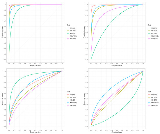
Figure 11.
ROC curves for the proposed (NEW), Gnedenko (GN), Gini (GI) and Shapiro–Wilk (SW) tests. No threshold, (left), and 70th percentile of the exponential distribution, (right). Data from Weibull, shape = 1.5 (Top) and from Gamma, shape = 0.8 (bottom) with n = 100.
Figure 12 provides the ROC curves for the new test for with six different thresholds including the entire data set (Q0). The left part of the figure refers to data from the Weibull distribution with shape = 1.5, while the right part refers to data from the Gamma distribution with a shape parameter taken to be equal to 0.8. The two cases cover log-convex as well as log-concave random variables with one chosen to be relatively close to the exponential distribution (Gamma with shape = 0.8) and the other slightly further away (Weibull shape = 1.5). Similar results have been obtained (results not shown) for different shape parameters ranging from to and from to for both the Gamma and the Weibull distributions with analogous results. Note further that although the results presented for both the size and power involve samples of size 100, the same results have been established for smaller samples sizes (), but due to space limitations, they cannot all be included in the manuscript. Note that the results for the Gamma case are not as exceptional as the ones for the Weibull case, but the proposed test is quite satisfactory as compared to other competitive tests, as Figure 11 shows.
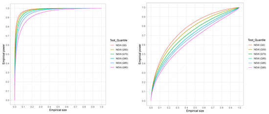
Figure 12.
ROC curves for the proposed test (NEW)—various thresholds of the exponential distribution—Weibull, shape = 1.5 (left), Gamma, shape = 0.8 (right), n = 100.
4. A Real Case Application
In this section, we wish to apply the proposed methodology to the Fire Insurance Danish data (Pfaff et al. 2012) with and show that the underlying distribution is a heavy-tailed one, which will be done based on Theorem 1. For illustrative purposes, the 50 values of the statistic given in (10) for permutations and various d values are presented in Figure 13 (blue bullets). The test statistic given in (12) is also depicted in the same figure (orange bullet).
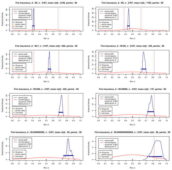
Figure 13.
Danish Fire Insurance Data—Test Statistic—50 permutations—.
Figure 13 clearly shows that the data exhibit eventually a heavy-tail part. Indeed, observe in Figure 13 that the values of the test statistic move to the right as the threshold d increases (i.e., as it attempts to reach infinity as per Equation (6)). It should be pointed out that for d equal to 99.7 or even 99.99, the value of is significantly large (over 300), which implies that the tail part of the distribution has not yet been reached, and as a result, the threshold d should be further increased to be able to capture the nature of the tail part of the distribution. Indeed, as the analysis of the fire insurance data shows, values at least equal to reveal a heavy-tail distribution, although a larger threshold may be needed for a statistically significant conclusion (as per Theorem 1). Finally, by implementing Theorem 1 with , and , the standardized test statistic is equal to and the exponentiality is rejected at a level of significance.
This data set clearly shows that when the focus is exclusively on the tail part, the choice of an ideal threshold is vital for accurate inferences. In reality, the proposed procedure succeeds in identifying the ideal finite value of d, which performs as accurately as the limiting result of (6) (or (5) for the case of a light-tailed distribution. The usefulness of the proposed methodology is evident if one notices that all available exponentiality tests in the literature are not capable of identifying the underlying distribution (like in the case of the fire insurance data), since as opposed to the proposed test, they are based on the entire data and fail, incorctly, to reject the null hypothesis.
5. Concluding Remarks
Conclusively, in this work, we focus on the distinction between the exponential distribution and distributions with log-concave or log-convex densities, i.e., with variables with light-tailed or heavy-tailed distributions, when the emphasis is placed exclusively on the tail part of the distribution, ignoring the rest of the distribution. We first identified a special characterization of the exponential distribution according to which the conditional random variable given in (4) separates the exponential random variable from log-convex and log-concave random variables. This is completed by focusing exclusively on a subset of the original dataset lying over a proper threshold (i.e., on the extreme portion of data), which is equal to at least the 90th percentile of the distribution for medium to large sample sizes and between the 75th and the 90th percentile for small sample sizes. In fact, this variable is centered around one-half () for the extreme part of an exponential random variable, with values above or below one-half for the extreme parts of log-convex and log-concave random variables, respectively. Then, the sample equivalent of the expectation of the above conditional random variable given in (10) was used to set up a novel goodness of fit test, the capabilities of which have been discussed by providing a detailed discussion about the choice of the proper threshold d (Section 3.2.3) and the pairing (Section 3.2.2). Both these issues provide the appropriate conditions and pave the way for the implementation of the test statistic, the performance of which has been investigated in terms of the size and the power and found to be robust for most practical purposes.
In conclusion, the proposed test appears to provide a valuable tool in the researcher’s toolbox for handling successfully the analysis of extreme events, some typical applications of which include the analysis of the magnitude of earthquakes, temperatures, floods or the insurance claims over a certain threshold, like the fire insurance data used in this work. One of the main contributions of the present work to the analysis of extreme events is that as opposed to classical tests based on the entire data set which often fail (incorrectly) to reject a null hypothesis, the proposed testing procedure checks the fit of the tail and makes the correct decision relying exclusively on the available data falling within the tail part of the distribution.
Author Contributions
Conceptualization, I.V. and A.K.; methodology, I.V., G.P. and A.K.; software, I.M. and G.P.; validation, I.M. and G.P.; formal analysis, I.M. and G.P.; investigation, I.M. and G.P.; resources, I.M. and G.P.; data curation, I.M. and G.P.; writing—original draft preparation, I.M. and A.K.; writing—review and editing, I.V., A.K., I.M. and G.P.; visualization, I.M.; supervision, A.K. All authors have read and agreed to the published version of the manuscript.
Funding
This research received no external funding.
Data Availability Statement
The fire insurance danish data are available at: https://utstat.utoronto.ca/sheldon/DataandCodes.html (accessed on 14 September 2023).
Acknowledgments
The authors wish to express their appreciation to the anonymous referees and the Associated Editor for their valuable comments and suggestions that greatly improved both the quality and the presentation of the manuscript. This work was completed as part of research activities of the Laboratory of Statistics and Data Analysis of the University of the Aegean.
Conflicts of Interest
The authors declare no conflict of interest.
Correction Statement
This article has been republished with a minor correction to resolve spelling and grammatical errors. This change does not affect the scientific content of the article.
References
- Ascher, Steven. 1990. A survey of tests for exponentiality. Communications in Statistics Theory and Methods 19: 1811–25. [Google Scholar] [CrossRef]
- Asmussen, Søren, and Jaakko Lehtomaa. 2017. Distinguishing log-concavity from heavy tails. Risks 5: 10. [Google Scholar] [CrossRef]
- Bagdonavičius, Vilijandas, Mikhail Nikulin, and Ruta Levuliene. 2013. On the Validity of the Weibull-Gnedenko Model. In Applied Reliability Engineering and Risk Analysis: Probabilistic Models and Statistical Inference. Edited by Ilia B. Frenkel, Alex Karagrigoriou, Anatoly Lisnianski and Andre Kleyner. Chichester: Wiley, pp. 259–74. [Google Scholar]
- Baratpour, S., and A. Habibi Rad. 2012. Testing goodness-of-fit for exponential distribution based on cumulative residual entropy. Communications in Statistics Theory and Methods 41: 1387–96. [Google Scholar] [CrossRef]
- Bryson, Maurice C. 1974. Heavy-tailed distributions: Properties and tests. Technometrics 16: 61–68. [Google Scholar] [CrossRef]
- Chhikara, Raj S., and J. Leroy Folks. 1977. The inverse Gaussian distribution as a lifetime model. Technometrics 19: 461–68. [Google Scholar] [CrossRef]
- Csorgo, Miklós, and Masoud M. Nasari. 2013. Asymptotics of randomly weighted u- and v-statistics: Application to bootstrap. Journal of Multivariate Analysis 121: 176–92. [Google Scholar] [CrossRef]
- Fisher, Ronald Aylmer, and Leonard Henry Caleb Tippett. 1928. Limiting forms of the frequency distribution of the largest and smallest member of a sample. Mathematical Proceedings of the Cambridge Philosophical Society 24: 180–90. [Google Scholar] [CrossRef]
- Foss, Serguei, Takis Konstantopoulos, and Stan Zachary. 2007. Discrete and continuous time modulated random walks with heavy-tailed increments. Journal of Theoretical Probability 20: 581–612. [Google Scholar] [CrossRef]
- Gail, Mitchell H., and Joseph L. Gastwirth. 1978. A scale-free goodness-of-fit test for the exponential distribution based on the Gini statistic. Journal of the Royal Statistical Society Series B: Statistical Methodology 40: 350–57. [Google Scholar] [CrossRef]
- Gnedenko, Boris. 1943. Sur la distribution limite du terme maximum d’une serie aleatoire. Annals of Mathematics 44: 423–53. [Google Scholar] [CrossRef]
- Gupta, Ramesh C., and Narayanaswamy Balakrishnan. 2012. Log-concavity and monotonicity of hazard and reversed hazard functions of univariate and multivariate skew-normal distributions. Metrika 75: 181–91. [Google Scholar] [CrossRef]
- Henze, Norbert, and Simos G. Meintanis. 2005. Recent and classical tests for exponentiality: A partial review with comparisons. Metrika 61: 29–45. [Google Scholar] [CrossRef]
- Huber-Carol, Catherine, and Ilia Vonta. 2004. Frailty models for arbitrarily censored and truncated data. Lifetime Data Analysis 10: 369–88. [Google Scholar] [CrossRef]
- Huber-Carol, Catherine, N. Balakrishnan, M. S. Nikulin, and M. Mesbah. 2002. Goodness-of-Fit Tests and Model Validity. Boston: Birkhauser. [Google Scholar]
- Jimenez-Gamero, M. Dolores, and Apostolos Batsidis. 2017. Minimum distance estimators for count data based on the probability generating function with applications. Metrika 80: 503–45. [Google Scholar] [CrossRef]
- Jureckova, Jana, and Jan Picek. 2001. A class of tests on the tail index. Extremes 4: 165–83. [Google Scholar] [CrossRef]
- Karagrigoriou, Alex, Georgia Papasotiriou, and Ilia Vonta. 2022. Goodness of fit exponentiality test against light and heavy tail alternatives. In Statistical Modeling of Reliability Structures and Industrial Processes. Edited by Ioannis S. Trianntafyllou and Mangey Ram. Boca Raton: CRC Press and Taylor and Francis, pp. 25–38. ISBN 9781032066257. [Google Scholar]
- Kim, Moosup, and Sangyeol Lee. 2016. On the tail index inference for heavy-tailed GARCH-type innovations. Annals of the Institute of Statistical Mathematics 68: 237–67. [Google Scholar] [CrossRef]
- Lehtomaa, Jaakko. 2015. Limiting behaviour of constrained sums of two variables and the principle of a single big jump. Statistics & Probability Letters 107: 157–63. [Google Scholar]
- Novikov, Alexey, Ruslan Pusev, and Maxim Yakovlev. 2015. Tests for Exponentiality, Tests for the Composite Hypothesis of Exponentiality, Package ‘Exptest’, CRAN. Available online: http://cran.nexr.com/web/packages/evir/evir.pdf (accessed on 14 September 2023).
- Papasotiriou, Georgia. 2021. Non Parametric Test for the Exponential Distribution. Master’s thesis, Department of Mathematics, National Technical University of Athens, Athens, Greece. Available online: https://dspace.lib.ntua.gr/xmlui/handle/123456789/53900 (accessed on 14 September 2023).
- Pfaff, Bernhard, Eric Zivot, Alexander McNeil, and Alec Stephenson. 2012. evir: Extreme Values in R. 2012. R Package Version 1.7-3. Available online: https://cran.r-project.org/web/packages/evir/evir.pdf (accessed on 14 September 2023).
- Rogozhnikov, Andrey P., and Boris Yu Lemeshko. 2012. A Review of tests for exponentiality. Paper presented at the 2012 IEEE 11th International Conference on Actual Problems of Electronics Instrument Engineering (APEIE), Novosibirsk, Russia, October 2–4; pp. 159–66. [Google Scholar]
- Rosalsky, Andrew, and Deli Li. 2017. A central limit theorem for bootstrap sample sums from non-i.i.d. models. Journal of Statistical Planning and Inference 180: 69–80. [Google Scholar] [CrossRef]
- Shapiro, Samuel S., and M. B. Wilk. 1972. An analysis of variance test for the exponential distribution (complete samples). Technometrics 14: 355–70. [Google Scholar] [CrossRef]
- Tremblay, Luc. 1992. Using the Poisson inverse Gaussian in bonus-malus systems. ASTIN Bulletin International Actuarial Association 22: 97–106. Available online: http://www.casact.org/library/astin/vol22no1/97.pdf (accessed on 14 September 2023). [CrossRef]
- Vonta, Filia, Kyriacos Mattheou, and Alex Karagrigoriou. 2012. On properties of the (ϕ, a)-power divergence family with applications in goodness of fit tests. Methodology and Computing in Applied Probability 14: 335–56. [Google Scholar] [CrossRef]
Disclaimer/Publisher’s Note: The statements, opinions and data contained in all publications are solely those of the individual author(s) and contributor(s) and not of MDPI and/or the editor(s). MDPI and/or the editor(s) disclaim responsibility for any injury to people or property resulting from any ideas, methods, instructions or products referred to in the content. |
© 2023 by the authors. Licensee MDPI, Basel, Switzerland. This article is an open access article distributed under the terms and conditions of the Creative Commons Attribution (CC BY) license (https://creativecommons.org/licenses/by/4.0/).