Abstract
Four deep generative methods for time series are studied on commodity markets and compared with classical probabilistic models. The lack of data in the case of deep hedgers is a common flaw, which deep generative methods seek to address. In the specific case of commodities, it turns out that these generators can also be used to refine the price models by tackling the high-dimensional challenges. In this work, the synthetic time series of commodity prices produced by such generators are studied and then used to train deep hedgers on various options. A fully data-driven approach to commodity risk management is thus proposed, from synthetic price generation to learning risk hedging policies.
1. Introduction
Whether for pricing, market stress testing or market risk measurement, time series are widely used in finance. For pricing, most of the proposals in the literature focus on the design of stochastic models, among which one can cite the famous Schwartz (1997) or Schwartz and Smith (2000). A comprehensive survey of stochastic models for commodities is proposed in Deschatre et al. (2021). However, the design of a model is expensive, and once a model is available it remains to tackle the tedious task of its calibration. Also, most of these approaches usually cannot be updated quickly when market conditions change as this task requires in-depth expertise.
Other arguments advocate even more for a change in the way commodity prices are simulated. Firstly, the number and diversity of time series to be simulated increases with the emergence of renewable energies and new markets, making the model design even more complex. Secondly, the need for a joint simulation of prices and volumes arises when using stochastic control tools based on machine learning and able to consider a large class of models in high-dimension (Fecamp et al. 2020). Recent successive crisis (sanitary, Texan), where consequences are especially observed on commodity prices, advocates also for the fast adaptation of models to new market conditions.
Deep generative methods for computer vision (Goodfellow et al. 2014; Kingma and Welling 2013) allows to hope for purely data-driven time series simulators, designed to be more flexible and realistic. Especially, the literature on these methods for time series has particularly benefited from the Generative Adversarial Networks (GANs) community, due to its ease of use and remarkable results on images. Dedicated neural network architectures designed to learn temporal dependencies were first proposed (Esteban et al. 2017; Mogren 2016; van den Oord et al. 2016; Wiese et al. 2020). To help the generator capture temporal dynamics or conditional distributions, some other proposals embed the series in a latent space. Yoon et al. (2019) propose to transform the time series in a supervised manner on a lower dimensional space on which a GAN is applied. This method lies in particular on the simultaneously training of the GAN and the latent space and necessitates five neural networks. Ni et al. (2020) use a theoretically grounded path transformation based on the signature to extract significant features of the trajectories, avoiding the need of learning the representation of the series. Methods based on a Stochastic Differential Equation (SDE) formulation of the sequences have also been introduced to help the generator (Kidger et al. 2021; Remlinger et al. 2022). Another approach consists in designing objective functions which take into account the temporal structure, such as conditional distribution between time steps (Remlinger et al. 2022; Xu et al. 2020). Some attempts to apply generative methods to time series simulating electric power scenarios have already been proposed. The synthetic power generations can be used for the operation and planning of power systems (Qiao et al. 2020). In Chen et al. (2018), the generator is conditioned to weather events, such as high wind days, and to the time of year to produce the generated samples.
Synthetic time series can be used in risk management, portfolio structuring and, last but not least, for risk hedging strategies. In particular, the samples from the generators can be used to hedge an option on derivatives. Deep hedging offers more flexibility concerning the risk criteria and can tackle high-dimensional problems (Fecamp et al. 2020). Machine learning for option pricing and hedging started in the early 1990s. Hutchinson et al. (1994) replicated the Black-Scholes option pricing with a neural network in a supervised approach. Since then, many works focused on flexibility brought by machine learning models (Bayer et al. 2019; Ferguson and Green 2018; Jacquier and Oumgari 2019; McGhee 2018; Vidales et al. 2018). The data-driven approach is supposed to be more adapted to market modeling, by lifting some of the strong assumptions of classical probabilistic models. However, the non-stationarity of the financial market remains an obstacle to the application of these methods. A complete literature review about machine learning for option pricing and hedging is proposed in Ruf and Wang (2020). Such deep hedgers need a large data set to be properly trained. Deep generative methods provide a way to address the lack of real data and promise realistic modeling. However, it is not clear in the literature how both cohabit, and how a fully unsupervised chain performs compared to classical methods.
In this article, four state-of-the-art deep generators for time series are compared on commodities including electricity, gas, coal and fuel. Some evaluation criterion are introduced to quantify the synthetic prices fidelity beyond the classical metrics from the literature. These synthetic time series are then used to train a deep hedger on call options and spread options. The replication loss of the different hedging strategies proposed by the deep hedgers are considered as evaluation metric of the usefulness of the generator. Through this approach, a purely data-driven method for risk management is provided, including commodity price modeling and risk hedging.
Contributions:
- Deep Generation: An numerical comparison of deep generative models is performed on commodity futures. Deep generators are more faithful than classical Geometric Brownian Motion baseline, and perform better on volatile markets.
- Deep Hedging: A hedging comparison on several options is provided, and designs outline for a purely unsupervised method for risk management. The accuracy of the deep hedger can be seen as an evaluation metric of the time series generators.
2. Generative Methods for Time Series
2.1. Deep Generative Models
Four time series generators are considered. They differ by the way in which the synthetic data are constructed, either focusing on learning representations of the series or on designing a temporal dedicated objective function.
2.1.1. Conditional Loss Euler Generator
Conditional Loss Euler Generator (CEGEN Remlinger et al. (2022)) relies on a SDE representation of the time series and minimizes a conditional distance between transition distributions of the real and generated sequences. The stochastic process formulation helps the generator to build the series while the conditional loss ensures the fidelity of the generations. The authors provide theoretical error bounds on the estimation of the diffusion parameters. In opposition to most of the proposals in the literature, CEGEN does not rely on a GAN framework and requires a single neural network.
Time series are seen as realisations of a diffusion on a period :
where is the drift, is the volatility, W is a d-dimensional Brownian motion and d indicates the dimension of the multivariate time series. In practice, a discrete approximation of the SDE is applied with a Euler scheme on a regular time grid with meshsize . The generator learns the functions and so that the synthetic process follows the same distribution as the target one X. The deep Euler scheme obtained is described as:
where is the drift estimation, is the volatility estimation and are i.i.d. random variables.
The authors introduce the conditional loss to address the issues of learning only marginals and the difficulty that recurrent neural networks have to properly capture temporal dependencies (Yoon et al. 2019). To do so, the Bures-Wasserstein-2 (Bhatia et al. 2019) is minimised at each time step between the conditional distributions. Then, the loss function is summed over the time steps:
By doing so, the generator is able to learn the distribution around each data point of the space at each time step, and provides better empirical results in terms of temporal accuracy than GAN-based methods (Remlinger et al. 2022). However, the SDE formulation loses generality and relies on Markovian and Gaussian assumptions.
2.1.2. Causal Optimal Transport GAN
Causal Optimal Transport GAN (COTGAN, Xu et al. (2020)) considers an adapted Wasserstein distance to continuous time processes (Backhoff-Veraguas et al. 2020). The generator extends the regularised approach of the Wasserstein distance of Genevay et al. (2018) to Causal Optimal Transport by adding a penalisation on the traditional cost function. Two discriminator networks learn to penalise anticipatory transport plans and thus ensure the temporal causality constraint. This model is theoretical sounded, easy to implement and demonstrates less bias in learning than other GANs for time series (Chris et al. 2018; Yoon et al. 2019).
In COTGAN, the authors use the Sinkhorn algorithm (Cuturi 2013) to compute the optimal transport plan between two probability distribution and :
where c is the cost function, H is the entropy regularisation of the transport plan with . The distance is minimized, to gain stability COTGAN considers the Sinkhorn divergence instead as an objective function, which also compares samples of the same distribution (Genevay et al. 2018).
In order to penalise non-causal transport plans, avoiding that current values depend on future values, a term is added to the classical cost function:
where are functions required in the Adapted Wasserstein distance formulation and truncated at a fixed J. In COTGAN, are approximated by two neural networks of parameter , which are trained to find the functions that increase the cost when the transport plans are not causal. Thus, the generator minimise the global Wasserstein distance, while the discriminators maximise the distance, as in a GAN framework.
2.1.3. Signature GAN
Signature GAN (SIGGAN, Ni et al. (2020)) introduces a conditional Auto-Regressive Feed-forward Neural Network (AR-FNN) for the generator, combined with signature embedding. AR-FNN is a network architecture dedicated to learning the sequence structure and which transforms past real time series and noise into future synthetic values. The theory-based Signature representation of the series (Chevyrev and Kormilitzin 2016) uniquely characterizes any continuous function by extracting the path characteristics.
A signature of a path X is defined as , where
where J is a compact time interval. The truncated signature of of order N is denoted . The lower order signature terms capture the overall description of the path, such as the mean or volatility. An interesting point with the signature framework is that two paths with the same signature means lead to having the same distribution. This theoretical guarantee allows minimising the difference between the signature means as an objective function for the generative task. The generator is an auto-regressive model estimating knowing . To estimate a neural network iterates the same process over time, and over the previous estimations. The loss function is the Wasserstein-1 distance (Villani 2008) between the real and fake distributions at time t:
where X indicates the real time series and the one obtained by the AR-FNN. The final objective function is then obtained by summing over each time steps and captures the conditional joint distribution of the time series signature. Unlike Wasserstein GAN (Arjovsky and Bottou 2017), there is no need to optimise a discriminator, as the conditional signature loss is used as a critic.
2.1.4. Time Series GAN
Time Series GAN (TSGAN, Yoon et al. (2019)) stands out by its specific training combining both supervised and unsupervised approaches. An embedding space is jointly learned with a GAN model to better capture the temporal dynamics. The generator thus produces sequences on a latent representation which are then reconstructed on the initial data space. By optimizing both supervised and adversarial objectives, the model takes advantage of the efficiency of GANs with a controllable learning approach.
A first neural network provide mappings e between real times series and a latent space:
is the static feature space, and is the temporal feature space. The embed spaces aims at facilitating the learning of temporal dependencies in a lower dimensional representation than the ground true ones , helping both the generator and the adversarial networks to learn significant features. The recovery function
returns the time series out of its latent representation and may be viewed as a decoder. The generator is a function g which takes as input some noise and outputs features into the latent spaces
The discriminator d operates from the feature space and outputs a classification score.
In this setup there is a joint objective. The first is to minimise the reconstruction loss, the embedding and recovery functions have to capture meaningful patterns of the time series in order to be useful for the generator. Secondly, unsupervised loss comes from the GAN framework where the generator minimises the distance between the discriminator outputs as the discriminator seeks to distinguish true from false features in a classification task. Relying only on a binary adversarial feedback might not be sufficient to retrieve conditional distribution. An additional supervised loss is provided to strengthen temporal distribution comprehension, and minimizes conditional distributions difference between real and synthetic data.
2.2. Metric Description
One well-known challenge in the time series generation community is the lack of efficient evaluation metrics (Eckerli 2021; Gao et al. 2020; Wang et al. 2021). To address this issue, one can provide a set of metrics to characterize the specific characteristics of the synthetic data. As done in Remlinger et al. (2022), three types of evaluation metrics are considered:
- Marginal metrics consider the Mean Squared Error (MSE) over time between statistics of real and synthetic samples. Statistics include average, 95% and 5% percentiles denoted respectively Avg, p95, p05. These metrics ensure that the marginal distributions are accurate across the period and quantify the quality of the overall time series envelop.
- The temporal dependency accuracy is measured with the MSE between quadratic variations (QVar) of the real and synthetic time series, approximated as
- Correlation structure (Corr) is evaluated with the average across time of the MSE between the terms of the covariance matrices of synthetic and reference sequences.
A new metric is introduced to evaluate the faithfulness of the generated prices based on the performance obtained by a deep hedger, detailed in Section 3.3.1. The deep hedger is trained on synthetic time series and the replication loss is compared to a classical risk hedging strategy. Some additional market based metrics are also proposed such as the Value-at-Risk (VaR) and the Expected Shortfall (ES).
3. Numerical Experiments
3.1. Joint Simulation of Futures
The prices considered consist of 3-month ahead (3 MAH) future contracts on the electricity, gas, oil and coal markets. Data is daily from 21 January 2020 to 31 December 2020 and comes from the French RTE database (https://www.rte-france.com/en/eco2mix/market-data, accessed on 20 August 2021). Deep generators produce 4-dimensional time series of 30 successive days. The underlying price law is assumed not to depend on the number of days left to maturity of the future contract. In practice, some variations are observed as maturity approaches. However, because the duration of the contract (3 months) is longer than the duration of simulation (30 days) the approximation is acceptable.
The Figure 1 reports the Maximum Likelihood Estimation (MLE) of the volatility and the correlation of a Geometric Brownian Motion (GBM Black and Scholes (1973)). A rolling window of 100 days is used to evaluate the dependency of these parameters with time.
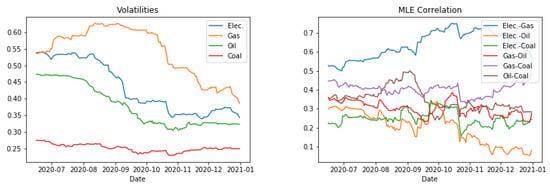
Figure 1.
Rolling mean of the volatility and correlation analysis of the commodity prices.
These parameters are not constant over time, highlighting the non-stationarity of the market and the difficulty of the calibration. For the sake of simplicity, an average approximation is done on these estimates for the calibration of the GBM (the deep generative methods are not concerned). The considered volatilities are , , and , and the correlation coefficients are
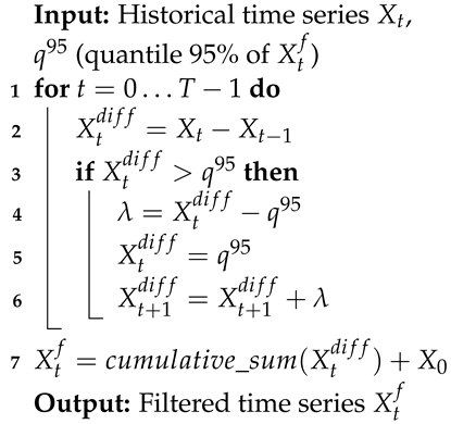
Commodity markets include stylised facts such as positive price jumps and heavy distribution tails. In order to facilitate the training of the generators, a filter is done on the data as pre-processing, described in Algorithm 1. By doing so, the trends of the original time series are preserved while avoiding extreme jumps.
| Algorithm 1: Jump Filter |
 |
3.2. Synthetic Prices
Table 1 reports the performance of the four generators on three types of evaluation metrics, alongside a 4-dimensional GBM calibrated on the historical dataset. The deep generative approaches provide better estimates of the marginal distributions than the GBM on every dimensions of the time series. CEGEN and TSGAN stand out and produce the most faithful time series. The time marginals are well estimated by CEGEN, without any high error value, emphasis that the global envelop is well respected. On the temporal aspects, SIGGAN and COTGAN provide consistent QVar depending on the considered dimension. In particular, the signature embedding preserves better the temporal structure than the other methods, especially on the gas dimension. Despite the low scores, CEGEN struggles with the Oil price temporal dependencies. As the SDE formulation is imposed on the generator, this result may express that Oil price dynamic may be not characterized with this diffusion. In the case of COTGAN, its adversarial loss performs well on the marginals but fails to replicate the temporal structure by flattening the time series as shown in Figure 2. TSGAN remains consistent on both marginal and transitional distributions, while being more general than CEGEN (which imposes a SDE formulation). The generative methods manage to properly capture the average correlation between electricity, gas, oil and coal. Especially, each generator outperforms the GBM simulations, and CEGEN relying on a similar SDE formulation as GBM returns the lowest correlation error. The evaluation of the calibrated GBM highlights that probabilistic models can be effective to model such time series. However, on the temporal aspects the GBM does not seem adapted. In practice, transfer learning could be a way to improve the training of deep generators, by first considering synthetic series and then refining the model with historical data.

Table 1.
Evaluation metrics on joint simulation of electricity, natural gas, coal and oil 3-month futures contracts prices. For all metrics, the lower, the better. Bold values indicate best metrics.
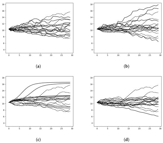
Figure 2.
Generation of the 3MAH Gas. Dashed lines represent trajectories of the historical time series, full lines represent samples produced by the generators. (a) CEGEN. (b) TSGAN. (c) COTGAN. (d) SIGGAN.
At this stage, CEGEN and TSGAN stand out for their faithful scenario price generations. However, it is not clear whereas these generators are accurate enough to be applied in an operational way.
3.3. Hedging Related Tests
The samples from the previously tested generators are used to (deep) hedge options on commodity derivatives. By comparing the replication errors on the basis of historical data, these numerical tests allow to go beyond the classical market statistics by comparing the different generators on an operational problem.
3.3.1. Deep Hedging
A self-financing strategy is a d-dimensional -adapted process on some probability space , where is the terminal date. Some market prices valued on of an underlying asset are given and observed on a discrete time grid , where is the spot. For the sake of simplicity, the time grid is assumed regular with mesh size . The terminal value of the portfolio at time is and defined as:
where will be referred to as the premium. The portfolio is re-balanced every day. There are no controls at the last date. A global approach is considered to learn the optimal policies as done in Fecamp et al. (2020), minimising a global criteria, in opposition of local schemes (reviewed in Germain et al. (2021)). A contingent claim pays at time T. The risk hedging problem leads to the following optimization problem
where the function ℓ indicates the quadratic loss and the payoff.
The optimal policy is approximated by a feed-forward neural network, called deep hedger. The model learns the optimal controls which minimise a hedging risk at the terminal value T. The network consists in 3 hidden layers of 10 units each with Relu activation. Adam optimizer is used, with learning rate at 1 × 10. The number of iterations is 10.000 and batch size is 300. There are four deep hedgers as there are four generators, each hedgers being trained on the samples of a generator. During the training, at each iteration of the deep hedger the generators simulate new data. The training set includes 211 historical price sequences of 30 dates on where the different evaluation scores are computed. The four different hedging policies are then tested on unobserved price time series from the historical data set. Figure 3 illustrates the full data-driven methods for risk hedging.
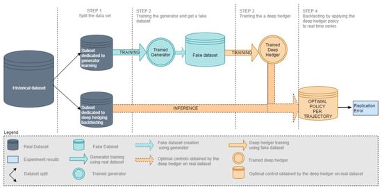
Figure 3.
Model-free deep hedger framework.
The deep hedger is an approximation of the optimal policy that contributes to the replication error of the hedged portfolios. In order to dissociate the nature of the replication error, that may come either from the underlying model or from the hedging policy estimation, an additional deep hedger is trained on a calibrated GBM. These replication errors of the hedged portfolios are used to evaluate the accuracy of the generators. If the synthetic prices are sufficiently realistic, no significant gap in the replication should be observed between a hedging strategy applied on the simulations and on the historical time series.
3.3.2. Hedging Evaluation Metrics
Hedging strategies put emphasis to reduce losses at the expense of gains. In order to focus on the losses associated with the different strategies, some risk metrics such as VaR or ES are considered. The standard deviation is also considered, but can be misleading because high gains will increase its value. To evaluate how a hedging strategy reduces the error, a score called the hedging effectiveness is defined:
where RiskMetric quantifies the risk (i.e., the variations) of profit and loss (PnL). The score belongs to , the greater, the better, and measures the improvement of the risk by hedging a position. A score of 1 means that no losses are observed. The hedging effectiveness score is computed in two steps. First, historical scenarios allow to evaluate the PnL of the hedging strategy for each scenario path. This back-testing builds a distribution of the strategy PnL from the scenarios. Thereafter, the pre-defined risk measure is evaluated with respect to this PnL distribution and derives the hedging effectiveness score. Three risk measures are studied:
- Standard deviation (Stdev): Standard deviation measures the amount of variation of the values in samples.
- Value-at-Risk (VaR): VaR measures tail loss, and is defined as the loss level that shall not be exceeded with a certain confidence level during a certain period of time.
- Expected shortfall (ES): ES is an alternative to VaR, which gives the expected loss in the worst few cases for a certain confidence level.
However, the standard deviation treats the variations in profit and loss indifferently, while the primary interest of hedging is to reduce losses and VaR may underestimate tail risk when the extreme loss is huge despite low probability. Therefore, a set of metrics is considered and a mean is also included as a RiskMetric. For both VaR and ES a confidence level of 95% is chosen in the numerical results below.
3.3.3. Call Option Hedging
Deep hedgers are trained on synthetic data produced by the generative methods listed out in Section 2. The hedging occurs on a daily basis on an at-the-money call option of payoff . The Black-Scholes (BS) model (Black and Scholes 1973) derives a closed formula which is used as baseline for the replication loss and premium comparison, and should not be confused with GBM which is a deep hedger trained on GBM samples. The four options are separately hedged on each of the markets previously described with maturities days and strikes . Spots are respectively for electricity, for gas, for coal and for fuel. The training and testing losses of the deep hedgers are provided in Appendix A.
Table 2 reports the replication errors of deep hedgers back-tested on unobserved historical prices. Initial risk indicates the risk of the payoff without hedging. The deep hedging policies bring improvements on every options compared to the initial risk and the BS model. The policy learned with CEGEN samples provides a significant lower replication loss than every other methods. On the oil case however, the very specific case where CEGEN did not manage to get correct QVar (Table 1), the replication loss is significantly higher (and close to BS). COTGAN, SIGGAN and TSGAN have close results, improving against BS. In particular, COTGAN does not stand out despite the good performances from Table 1. The results with hedging options are consistent with the first analysis. CEGEN outperforms the other generators in most of the cases, even if every methods provide relevant hedging policies in terms of replication loss.

Table 2.
Replication losses of deep hedgers trained on synthetic data for 3MAH forwards (French market). Bold values indicate best scores.
Figure 4 illustrates the PnL distributions for each deep hedger trained on each generator, alongside with the distribution of the initial risk. TSGAN outperforms the other generators, by always being consistently in the top 2 of the least risky PnL distributions. CEGEN also presents high performances on every commodities, unlike the SIGGAN and the GBM which weaken on fuel, with notably a high tail risk.
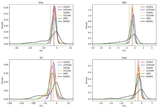
Figure 4.
PnL distributions for at-the-money call option hedging. Vertical lines represent the means of the associated distributions.
An options trader determines a selling price according to the hedging strategy of the PnL distribution. In order to be attractive in the market, the trader has to offer a low price, slightly higher than the average of the PnL distribution, to make a profit. However, if this distribution is too dispersed, the trader has to cover the risk of big losses by offering a higher price. In the case of fuel, using the GBM or SIGGAN strategies, the trader must not make a mistake by proposing a low price in spite of a significant recentering of the distribution around the average because the tail risk is very high. Another observation is that in all cases below, the vertical lines representing the averages of the different distributions are higher for the hedging strategies than for the naked strategy. However, under the assumption of no arbitrage, the average PnL should be the same when hedging or not. If this looks profitable, especially for the COTGAN whose averages are the highest, it is not necessarily a sign of good performance. On the contrary, it may be because of bad hedging evaluation, but in the context of a bullish market, it may turn to its advantage.
Table 3 reports the hedging ratios for the Stdev, VaR and ES risk metrics. At first sight, it seems difficult to distinguish the best generator. COTGAN outperforms sporadically the other methods, but TSGAN provides a better ratio with the Stdev metric. CEGEN has close results and stand out on the gas case. On these hedging scores, determining the best model is not sufficient, but analysing the controls obtained by the associated policies could allow a more in-depth comparison.

Table 3.
Hedging scores of at-the-money call options. For all scores, the closer to 1, the better. Bold values indicate best scores.
The controls from each model on a single historical price trajectory are illustrated in Figure 5. The policies of CEGEN and SIGGAN are very reactive to the price, and propose similar policy on each option. COTGAN as for it provides low volatility controls on electricity and gas data, in the opposite on oil and fuel the deep hedger seem to follow the price of the commodity. Such instability may question the validity of the policy, and would need further analysis. This is consistent with the Table 1 and the unrealistic smooth curves that did not have significant price fluctuations shown in the Figure 2. In all cases, TSGAN and BS controls are relatively consistent and appear to be unaffected by the price, buying the same amount of asset over time during the period.
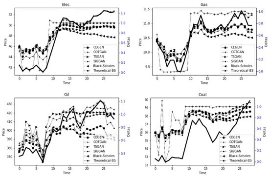
Figure 5.
Controls proposed by each risk hedging strategy. Full line represents a price time series. Dashed lines are the quantity of the underlying needed to hedge the risk at each time step.
The hedging results are closely related with the time series accuracy of Section 3.1, the strategies that stand out are the ones obtained from CEGEN and TSGAN. However, considering the hedging ratio as evaluation metric, COTGAN samples are the most realistic of the set of tested generators. When training the deep hedger, it seems that smooth price time series can be enough to learn an average strategy. A deep look on the obtained controls seems necessary.
3.3.4. Spread Option Hedging
A call option on the spread between gas and coal has a payoff . The spread is the price difference between these two commodities, where the strike is the initial spread . As in the previous section, the maturity remains 30 days and the hedge portfolio is rebalanced everyday. Although the success of the hedge still depends heavily on a correct representation of the gas and coal time series individually, this is no longer the only condition for learning a good strategy. Generators must also represent the joint distribution of these prices to correctly train a deep hedger on the spread. In particular, the generators’ appreciation of the historical correlation is crucial to the correct modelling of prices.
Table 4 reports the hedging effectiveness scores for the risk metrics alongside the PnL. Here, COTGAN and CEGEN outperform the other methods. However, in the case of COTGAN, the smooth price trajectories (illustrated in Figure 2) do not seem to affect the scores. In practice, such trajectories could not be used.

Table 4.
Hedging effectiveness of at-the-money call option on spread. Bold values indicate best scores.
Figure 6 highlights a significant difference between the CEGEN-based strategy and the others. A surprising result is TSGAN, which is ranked among the best generators, is now in third place. This is nevertheless consistent with Table 1 indicating a poor replication of the correlation.
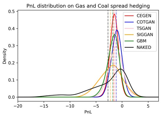
Figure 6.
PnL distribution for spread option hedging. Vertical dashed lines represent the mean of the distributions.
CEGEN seems to be the generator of choice for a case where the correlation between different time series has to be taken into account. However, despite the very good performance in the univariate hedging case, TSGAN fails to perform well in this situation.
4. Conclusions
This study describes a purely data-driven approach for risk management, from time series generation to hedging on commodity markets. A comparison between state-of-the-art deep generative methods is proposed on energy market applications. First, the accuracy of the generations is evaluated on energy commodity prices. Then, a study focuses on the usefulness of these generators in a risk hedging task. Deep hedgers are trained on synthetic data produced by the generators for several options. Deep generative methods outperform classical pricing approaches, the hedging performance aligns very closely with the generation fidelity. Among the deep generators, CEGEN and TSGAN stand out on tested commodities and for both market indicators and replication losses. While TSGAN provides more accurate time series, especially in terms of temporal structure, CEGEN is better at representing interdependencies in a joint simulation. The latter is more easily interpretable than TSGAN, but at the cost of reduced generality.
Author Contributions
Conceptualization, J.M. and C.R.; methodology, J.M. and C.R.; validation, N.B., C.R. and J.M.; formal analysis, N.B., C.R. and J.M.; investigation, N.B.; resources, J.M.; writing—original draft preparation, J.M., C.R. and N.B.; writing—review and editing, J.M., C.R. and N.B.; visualization, J.M., C.R. and N.B.; supervision, J.M. and C.R.; project administration, J.M. All authors have read and agreed to the published version of the manuscript.
Funding
This research received no external funding.
Data Availability Statement
Publicly available datasets were analyzed in this study. This data can be found here: https://www.rte-france.com/en/eco2mix/market-data, accessed on 20 August 2021.
Acknowledgments
This research is supported by the department OSIRIS (Optimization, SImulation, RIsk and Statistics for energy markets) of EDF Lab, by EDF Lab Singapore and by FiME laboratory which are gratefully acknowledged. We would like to thank Carol Hargreaves for her feedback.
Conflicts of Interest
The authors declare no conflict of interest.
Appendix A. Models and Hyper-Parameters
Our methodology follows the proposed in the respective papers concerning the choice of hyper-parameters and architecture of neural networks. The original code of the papers is used for our simulation, expecting for TSGAN where the version used is the one from the Conditional Signature GAN GitHub. The hyper-parameters tuning is performed using a gridsearch.
Appendix A.1. Model Specifications
Appendix A.1.1. CEGEN
The generator includes a single neural network. As proposed in Remlinger et al. (2022), a feed forward neural network is considered, composed of 2 layers of 3 times the data dimension each. Table A1 shows architectural and settings choice.

Table A1.
Generator neural network hyper-parameters for CEGEN.
Table A1.
Generator neural network hyper-parameters for CEGEN.
| Settings of CEGEN | |
|---|---|
| (ndates) | 30 |
| Optimizer | Adam |
| Training iterations | 1000 |
| Batch size | 300 |
| Learning rates | 1 × |
Appendix A.1.2. COTGAN
The generator is represented by 3-layer LSTM network, whose output at each time step is passed through a ReLU network. Adam is used for updating and , with learning rate 1 × . Batch size is 32. The discriminator is a network that has two layers of 1-D causal CNN with stride 1, filter length 5. Each layer has 32 neurons. The activation is ReLU for each layer except the output which is a sigmoid. Table A2 summarizes those parameters choices.

Table A2.
Generator neural network hyper-parameters for COTGAN.
Table A2.
Generator neural network hyper-parameters for COTGAN.
| Settings of COTGAN | |
|---|---|
| (ndates) | 30 |
| White noise dim | |
| Optimizer | Adam |
| Training iterations | 1000 |
| Batch size | 32 |
| Learning rates | 1 × |
Appendix A.1.3. SIGGAN and TSGAN
SIGGAN and TSGAN use the same AR-FNN generator in this paper. The structure uses 3 types of layers: feed forward, parametric rectified linear unit and residual layers. The two last terms are thus defined:
- parametric rectified linear unit (PReLU) is a parameterised function with ,
- Residual layer: let be an affine function, and a PReLU, the residual layer function is,
The generator is composed of one layer FNN followed by one PReLU and 2 residual layers, and one last FNN, as shown in Table A3. It takes as input the p last values of the d-dimensional time series that we simulate. Adam optimizer is used, the number iterations is 1000 during the training process. The learning rates are set at 1 × for SIGGAN and 3 × for TSGAN as prescribed in the introducing papers of the generators. TSGAN proposes 2 discriminator weights updates for 1 generator weight update to improve the convergence. SIGGAN does not have a discriminator network. TSGAN uses the same ARFNN architecture for the discriminator network.

Table A3.
Generator ARFNN settings.
Table A3.
Generator ARFNN settings.
| Settings of ARFNN | |
|---|---|
| (ndates) | 30 |
| Optimizer | Adam |
| Training iterations | 1000 |
| Batch size | 32 |
| Learning rates | 1 × (SIGGAN), 3 × (TSGAN) |
Appendix A.2. Convergence of Models
Appendix A.2.1. Deep Generation
As shown in Figure A1, all generators seem to converge, their losses reach a plateau.
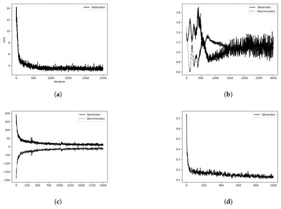
Figure A1.
Generators losses. Dotted lines represent discriminator losses; full lines represent generator losses. For CEGEN and SIGGAN there is no discriminator neural network. (a) CEGEN. (b) TSGAN. (c) COTGAN. (d) SIGGAN.
Appendix A.2.2. Deep Hedging
Hedging a Call Option
Figure A2 illustrates that the training and testing losses of the deep hedgers are closer in the CEGEN and TSGAN cases than in the GBM, COTGAN, and SIGGAN cases.
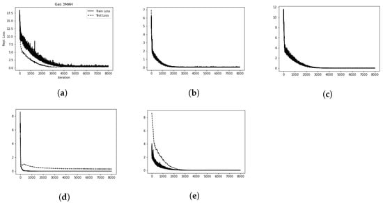
Figure A2.
Losses of the deep hedgers training on the 3 MAH Gas call option. Dashed lines represent test losses computed on the historical time series; plain lines represent generator losses computed on synthetic time series. (a) GBM (b) CEGEN. (c) TSGAN. (d) COTGAN. (e) SIGGAN.
Hedging a Spread Option
Figure A3 reports the replication errors of the deep hedgers trained on synthetic prices to hedge a spread option. For all models, the convergence is quickly reached, but the replication losses of the hedgers based on TSGAN and SIGGAN is more volatile, which can be due to their specific time series embedding.
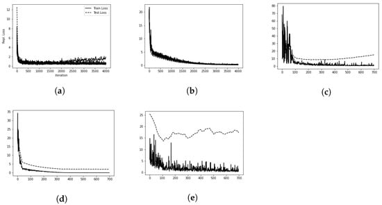
Figure A3.
Losses of the deep hedgers training to hedge a spread option between 3MAH Gas and 3MAH Coal. Dashed lines represent test losses computed on the historical time series; plain lines represent generator losses computed on synthetic time series. (a) GBM (b) CEGEN. (c) TSGAN. (d) COTGAN. (e) SIGGAN.
References
- Arjovsky, Martin, and Léon Bottou. 2017. Towards principled methods for training generative adversarial networks. arXiv arXiv:1701.04862. [Google Scholar]
- Backhoff-Veraguas, Julio, Daniel Bartl, Mathias Beiglböck, and Manu Eder. 2020. Adapted wasserstein distances and stability in mathematical finance. Finance and Stochastics 24: 601–32. [Google Scholar] [CrossRef]
- Bayer, Christian, Blanka Horvath, Aitor Muguruza, Benjamin Stemper, and Mehdi Tomas. 2019. On deep calibration of (rough) stochastic volatility models. arXiv arXiv:1908.08806v1. [Google Scholar]
- Bhatia, Rajendra, Tanvi Jain, and Yongdo Lim. 2019. On the bures–wasserstein distance between positive definite matrices. Expositiones Mathematicae 37: 165–91. [Google Scholar] [CrossRef]
- Black, Fischer, and Myron Scholes. 1973. The pricing of options and corporate liabilites. Journal of Political Economy 81: 637–54. [Google Scholar] [CrossRef]
- Chen, Yize, Yishen Wang, Daniel Kirschen, and Baosen Zhang. 2018. Model-free renewable scenario generation using generative adversarial networks. IEEE Transactions on Power Systems 33: 3265–75. [Google Scholar] [CrossRef]
- Chevyrev, Ilya, and Andrey Kormilitzin. 2016. A primer on the signature method in machine learning. arXiv arXiv:1603.03788. [Google Scholar]
- Chris, Donahue, McAuley Julian, and Miller Puckette. 2018. Adversarial audio synthesis. arXiv arXiv:1802.04208. [Google Scholar]
- Cuturi, Marco. 2013. Sinkhorn distances: Lightspeed computation of optimal transport. arXiv arXiv:1306.0895. [Google Scholar]
- Deschatre, Thomas, Olivier Féron, and Pierre Gruet. 2021. A survey of electricity spot and futures price models for risk management applications. Energy Economics 102: 105504. [Google Scholar] [CrossRef]
- Eckerli, Florian. 2021. Generative adversarial networks in finance: An overview. SSRN 3864965. [Google Scholar] [CrossRef]
- Esteban, Cristóbal, Stephanie L. Hyland, and Gunnar Rätsch. 2017. Real-valued (medical) time series generation with recurrent conditional gans. arXiv arXiv:1706.02633. [Google Scholar]
- Fecamp, Simon, Joseph Mikael, and Xavier Warin. 2020. Deep learning for discrete-time hedging in incomplete markets. Journal of Computational Finance 25: 51–85. [Google Scholar] [CrossRef]
- Ferguson, Ryan, and Andrew Green. 2018. Deeply learning derivatives. arXiv arXiv:1809.02233. [Google Scholar]
- Gao, Nan, Hao Xue, Wei Shao, Sichen Zhao, Kyle Kai Qin, Arian Prabowo, Mohammad Saiedur Rahaman, and Flora D. Salim. 2020. Generative adversarial networks for spatio-temporal data: A survey. arXiv arXiv:2008.08903. [Google Scholar] [CrossRef]
- Genevay, Aude, Gabriel Peyré, and Marco Cuturi. 2018. Learning generative models with sinkhorn divergences. Paper presented at the Twenty-First International Conference on Artificial Intelligence and Statistics, Canary Islands, Spain, April 9–11; pp. 1608–17. [Google Scholar]
- Germain, Maximilien, Huyên Pham, and Xavier Warin. 2021. Neural networks-based algorithms for stochastic control and pdes in finance. arXiv arXiv:2101.08068. [Google Scholar]
- Goodfellow, Ian, Jean Pouget-Abadie, Mehdi Mirza, Bing Xu, David Warde-Farley, Sherjil Ozair, Aaron Courville, and Yoshua Bengio. 2014. Generative adversarial nets. Paper presented at the Conference Advances in Neural Information Processing Systems, Montréal, QC, Canada, December 8–13; pp. 2672–80. [Google Scholar]
- Hutchinson, James M., Andrew W. Lo, and Tomaso Poggio. 1994. A nonparametric approach to pricing and hedging derivative securities via learning networks. The Journal of Finance 49: 851–89. [Google Scholar] [CrossRef]
- Jacquier, Antoine Jack, and Mugad Oumgari. 2019. Deep ppdes for rough local stochastic volatility. SSRN 3400035. [Google Scholar] [CrossRef]
- Kidger, Patrick, James Foster, Xuechen Li, Harald Oberhauser, and Terry Lyons. 2021. Neural sdes as infinite-dimensional gans. arXiv arXiv:2102.03657. [Google Scholar]
- Kingma, Diederik P., and Max Welling. 2013. Auto-encoding variational bayes. arXiv arXiv:1312.6114. [Google Scholar]
- McGhee, William. 2018. An artificial neural network representation of the sabr stochastic volatility model. SSRN 25: 3984219. [Google Scholar] [CrossRef]
- Mogren, Olof. 2016. C-rnn-gan: Continuous recurrent neural networks with adversarial training. arXiv arXiv:1611.09904. [Google Scholar]
- Ni, Hao, Lukasz Szpruch, Magnus Wiese, Shujian Liao, and Baoren Xiao. 2020. Conditional sig-wasserstein gans for time series generation. arXiv arXiv:2006.05421. [Google Scholar] [CrossRef]
- Qiao, Ji, Tianjiao Pu, and Xinying Wang. 2020. Renewable scenario generation using controllable generative adversarial networks with transparent latent space. CSEE Journal of Power and Energy Systems 7: 66–77. [Google Scholar]
- Remlinger, Carl, Joseph Mikael, and Romuald Elie. 2022. Conditional loss and deep euler scheme for time series generation. Paper presented at the 36th AAAI Conference on Artificial Intelligence, Vancouver, BC, Canada, February 22–March 1; pp. 8098–8105. [Google Scholar]
- Ruf, Johannes, and Weiguan Wang. 2020. Neural networks for option pricing and hedging: A literature review. arXiv arXiv:1911.05620. [Google Scholar] [CrossRef]
- Schwartz, Eduardo. 1997. The stochastic behavior of commodity prices: Implications for valuation and hedging. The Journal of Finance 52: 923–73. [Google Scholar] [CrossRef]
- Schwartz, Eduardo, and James E. Smith. 2000. Short-term variations and long-term dynamics in commodity prices. Management Science 46: 893–911. [Google Scholar] [CrossRef]
- van den Oord, Aaron, Sander Dieleman, Heiga Zen, Karen Simonyan, Oriol Vinyals, Alex Graves, Nal Kalchbrenner, Andrew Senior, and Koray Kavukcuoglu. 2016. Wavenet: A generative model for raw audio. arXiv arXiv:1609.03499. [Google Scholar]
- Vidales, Marc Sabate, David Siska, and Lukasz Szpruch. 2018. Unbiased deep solvers for parametric pdes. arXiv arXiv:1810.05094. [Google Scholar]
- Villani, Cédric. 2008. Optimal Transport: Old and New. Berlin: Springer Science & Business Media, vol. 338. [Google Scholar]
- Wang, Zhengwei, Qi She, and Tomas E. Ward. 2021. Generative adversarial networks in computer vision: A survey and taxonomy. ACM Computing Surveys (CSUR) 54: 1–38. [Google Scholar] [CrossRef]
- Wiese, Magnus, Robert Knobloch, Ralf Korn, and Peter Kretschmer. 2020. Quant gans: Deep generation of financial time series. Quantitative Finance 20: 1419–40. [Google Scholar] [CrossRef]
- Xu, Tianlin, Li K. Wenliang, Michael Munn, and Beatrice Acciaio. 2020. Cot-gan: Generating sequential data via causal optimal transport. arXiv arXiv:2006.08571. [Google Scholar]
- Yoon, Jinsung, Daniel Jarrett, and Mihaela van der Schaar. 2019. Time-series generative adversarial networks. Paper presented at the Advances in Neural Information Processing Systems Conference, Vancouver, BC, Canada, December 8–14. [Google Scholar]
Disclaimer/Publisher’s Note: The statements, opinions and data contained in all publications are solely those of the individual author(s) and contributor(s) and not of MDPI and/or the editor(s). MDPI and/or the editor(s) disclaim responsibility for any injury to people or property resulting from any ideas, methods, instructions or products referred to in the content. |
© 2022 by the authors. Licensee MDPI, Basel, Switzerland. This article is an open access article distributed under the terms and conditions of the Creative Commons Attribution (CC BY) license (https://creativecommons.org/licenses/by/4.0/).