Heat Equation as a Tool for Outliers Mitigation in Run-Off Triangles for Valuing the Technical Provisions in Non-Life Insurance Business

Abstract

Estimating outstanding claims reserves in the non-life insurance business is often impaired by outlier-contaminated datasets. Widely used methods to eliminate outliers in non-life development triangles are either limiting the number of outliers by robust statistical methods or by change of development factors. However, the whole estimation process is likewise adversely affected so that: (i) the total sum of all triangle payments is not correct or (ii) the difference between the original triangle and its backward estimation via the bootstrap method is ineligible. In this paper, the properties of the heat equation are examined to obtain an outlier smoothing technique for development triangles. The heat equation in two dimensions is being applied on an outlier contaminated dataset where no individual data are available. As a result, we introduce a new methodology to (i) treat outliers in non-life development triangles, (ii) keep the total sum of all triangle payments, and (iii) provide acceptable differences between the original and the backward estimated triangle. Consequently, the outlying values are eliminated and the resulting development triangle could be used as an input for any claims reserving method without a need for further robustification or change of development factors. Additionally, the research on the application of heat equation in one dimension presented in this paper enables one to employ the bootstrap method using Pearson’s residuals in cases where the method was originally inapplicable due to development factors being lower than one.

1. Introduction

According to Solvency II regulations, the insurer must be able to estimate the future claims reserves as accurately as possible. The insurer who operates in the non-life insurance business often does not know the amount of the final claims for the year of the accident at the end of that year. It depends on the business line in the non-life insurance industry or the time duration of a claims settlement. Delays can occur due to the time lag between the occurrence of the accident and the appearance of the consequences of the event. Therefore, a run-off triangle can be considered to arrange the claims reserves. Most important is to estimate the outstanding claims reserve. Various methods can be used, the most popular one is the classic chain-ladder method (Verdonck et al. 2009).

“The chain ladder method is based on the assumption that the expectations underlying the columns and the rows in the run-off triangle are proportional” (Verdonck et al. 2009). Since the early 1990s, several articles have been published to incorporate the simple chain ladder method into the statistical framework, and consideration has been given to stochastic models that generate a chain ladder algorithm (Manolache 2019). Full stochastic models for the chain ladder method were published by (Liu and Verrall 2010; Mack 1993; Murphy 1994; Verdonck and Debruyne 2011; Verdonck et al. 2009) and other authors. Extended versions of these models have also been created. For example, (Peters et al. 2014) developed an extended class of model structures for the paid–incurred chain ladder models, where they developed exactly the Bayesian formulation of such models. (Wuthrich 2017) extended the chain-ladder method for claims reserving to include information about the properties of individual claims applying a neural network model. “The chain ladder method should only be used for large portfolios where consistency of the estimates is more important than unbiasedness and where all entries into the incurred loss triangle are rather reliable (no big relative chance fluctuations and/or errors)” (Bühlmann 2016, p. 7).

The Cape Cod method, which is also known as the Stanard–Buhlmann method, (Bühlmann and Straub 1983; Stanard 1985) was proposed to overcome some of the shortcomings of the chain ladder method (Saluz 2015). The a priori loss ratio in the Cape Cod method “is calculated as the weighted average of the chain ladder ultimate loss ratios across all years with the used premium as the weights” (Korn 2016, p. 1). Due to its simplicity and advantages over the chain ladder method, the Cape Cod method has become a proven method in practice (Saluz 2015). The Cape Cod method is a special case of the Generalized Cape Cod Methods addressed by (Gluck 1997; Korn 2016; Struzzieri et al. 1998).

A popular method that generates a simulated prediction distribution to obtain the standard errors of well-specified models is bootstrapping (Verdonck et al. 2009). This method has already been considered in the area of claims reserving by (England and Verrall 1999; Lowe 1994; Maciak et al. 2022; Zaçaj et al. 2022). Several authors (Peremans et al. 2017; Verdonck et al. 2009) applied robust bootstrap procedures for the chain-ladder method.

One of the key decisions in estimating claims reserves is how to treat outliers. According to (Embrechts and Wüthrich 2022, p. 5) outliers in insurance typically are not data errors but large financial claims that are an important pricing component. (Verdonck and Van Wouwe 2011) proposed two techniques to detect and correct outliers in the bivariate chain-ladder method—the first technique was based on the bagplot to the bivariate dataset and the second one was the robust technique based on the MCD (Minimum Covariance Determinant). (Avanzi et al. 2022) extended their approach and also applied two alternative robust bivariate chain-ladder techniques to treat outlier—the first one was based on the outlyingness and the second technique was based on bagdistance, which is derived from the bagplot.

In relation to the above-mentioned, the objective of designing an in-house application (Barlak 2021) for computing non-life reserves using well-defined deterministic and stochastic methods (Avanzi et al. 2016; Badounas and Pitselis 2020; Brazauskas et al. 2009; Peremans et al. 2018; Verdonck and Van Wouwe 2011; Verdonck et al. 2009), and challenges associated with the lack of person-specific data, lead us to the design of a new method to treat outliers in non-life development triangles. By applying properties of the heat equation, outliers could be treated without changing the whole triangle payments total sum. Furthermore, a bootstrap method using residuals could be applied in some cases where it was originally impossible.

The heat equation is a partial differential equation that describes temperature changes in a given area over a period of time (Gorguis and Chan 2008). The one-dimensional heat equation was first studied by Fourier at the beginning of the 19th century (Cannon and Browder 1984). The heat equation has applications in various fields of science, one of the most important of them is the theory of heat conduction (Widder 1976). It has also been used for image enhancement (Black and Sapiro 1999; Buades et al. 2006) or for a detection of a pollution problem (El Badia and Ha-Duong 2002). (Itkin et al. 2021) applied multi-layer heat equations when solving financial problems and developing efficient algorithms for pricing barrier options for time-dependent one-factor short-rate models. At present, we are not aware of the use of the heat equation to treat outliers in non-life development triangles. In this paper, we fill this gap by proposing a new method to treat outliers, which is based on a heat equation.

Based on the above, we set the aim of the paper to design a new method to treat outliers in non-life development triangles.

The remainder of the paper is structured as follows. Section 2 outlines the theoretical basis of methods for the calculation of technical reserves. Selected Chain-ladder and Cape Cod deterministic methods (Section 2.1.1) with their stochastic adjustments (Section 2.1.2) and additional stochastic modification (Cowell 2009) (Section 2.1.3) are introduced in this section. Two different methods for treating outliers in 2-D (Section 2.4.1 and Section 2.4.2) and an approach to the numerical solution of one- and two-dimensional heat equation (Section 2.2 and Section 2.3) constitute the core part of this research. Finally, a method for adjusting development factors to be greater than one (>1) without changing the total sum in a triangle row is proposed in this section, with description and real-world examples being presented. Section 3 lists the results of the practical application of the heat equation when treating outliers in non-life development triangles. Section 5 summarizes the essential conclusions resulting from the research and presents the significant findings.

2. Materials and Methods

2.1. Methods for Technical Reserves Calculation

Hereby, we would like to recall some concepts that underlie the technical reserves calculation briefly. For a detailed description, the interested reader could refer to (Avanzi et al. 2016; Badounas and Pitselis 2020; Brazauskas et al. 2009; Peremans et al. 2018; Verdonck and Van Wouwe 2011; Verdonck et al. 2009).

2.1.1. Deterministic Methods

Let us start with a brief overview of the well-known deterministic methods used for the calculation of technical reserves in this paper. We use two deterministic methods for the mentioned purposes. Firstly, it is the Chain-ladder method ${\widehat{C}}_{i,J}^{CL}=C_{i,I-i}·{\prod }_{k=I-i}^{J-1}\widehat{f_k}$, where $\widehat{f_j}={\sum }_{s=0}^{I-j-1}\frac{C_{s,j+1}}{{\sum }_{k=0}^{I-j-1}{C}_{i,k}}$ for I as maximum number of years from an event of a claim and J stands for the total number of development years. Secondly, we have chosen the Cape-Cod method using the following formula for technical reserves computation ${\widehat{C}}_{i,J}^{CC}=C_{i,I-i}+(1-\widehat{l_i})\widehat{\kappa }{P}_i$ (Dahms 2021), where $\widehat{\kappa }=\frac{{\sum }_{i=1}^I{C}_{i,I-i}}{{\sum }_{i=1}^I\widehat{l_i}{P}_i}$.

The choice for a stochastic process was subjectively the simplest one, namely the bootstrap. We have employed two modifications of the deterministic methods. The first one uses residuals.

2.1.2. Bootstrap Method Using Residuals

In general, we have a triangle of cumulative payments (

Table 1. Cumulative claim payments.

i\j	0	1	...	J-i	...	J-1	J
0	$C_{0,0}$	$C_{0,1}$	...	$C_{0,j}$	...	$C_{0,I-1}$	$C_{0,J}$
1	$C_{1,0}$	$C_{1,1}$	...	$C_{1,j}$		$C_{1,J-1}$
⋮			⋮		⋰
i	$C_{i,0}$	$C_{i,1}$	...	$C_{i,j}$
⋮			⋰
I-1	$C_{I-1,0}$	$C_{I-1,1}$
I	$C_{I,0}$

Source: own construction.

).

In the next step, we estimate development factors, which help us to calculate cumulative payments in the lower triangle (

Table 2. Completed lower triangle.

i\j	0	1	...	J-i	...	J-1	J
0	$C_{0,0}$	$C_{0,1}$	...		...	$C_{0,I-1}$	$C_{0,J}$
1	$C_{1,0}$	$C_{1,1}$	...			$C_{1,I-1}$	${\widehat{C}}_{1,J}$
⋮			⋮		⋰
i	$C_{i,0}$	$C_{i,1}$	...	$C_{i,J-i}$	...	${\widehat{C}}_{i,J-1}$	${\widehat{C}}_{i,J}$
⋮			⋰		⋮
I-1	$C_{I-1,0}$	$C_{I-1,1}$				${\widehat{C}}_{I-1,J-1}$	${\widehat{C}}_{I-1,J}$
I	$C_{I,0}$	${\widehat{C}}_{I,1}$	...		...	${\widehat{C}}_{I,J-1}$	${\widehat{C}}_{I,J}$

Source: own construction.

).

For the moment, we use the diagonal and apply the formula ${\widehat{C}}_{i,J}^{CL}=C_{i,I-i}·{\prod }_{k=I-i}^{J-1}\widehat{f_k}$ to estimate observed values of payments backwards (

Table 3. Estimated upper triangle backwards.

i\j	0	1	...	J-i	...	J-1	J
0	${\widehat{C}}_{0,0}$	${\widehat{C}}_{0,1}$	...		...	${\widehat{C}}_{0,I-1}$	$C_{0,J}$
1	${\widehat{C}}_{1,0}$	${\widehat{C}}_{1,1}$	...			$C_{1,I-1}$	${\widehat{C}}_{1,J}$
⋮			⋮		⋰
i	${\widehat{C}}_{i,0}$	${\widehat{C}}_{i,1}$	...	$C_{i,J-i}$	...	${\widehat{C}}_{i,J-1}$	${\widehat{C}}_{i,J}$
⋮			⋰		⋮
I-1	${\widehat{C}}_{I-1,0}$	${\widehat{C}}_{I-1,1}$				${\widehat{C}}_{I-1,J-1}$	${\widehat{C}}_{I-1,J}$
I	$C_{I,0}$	${\widehat{C}}_{I,1}$	...		...	${\widehat{C}}_{I,J-1}$	${\widehat{C}}_{I,J}$

Source: own construction.

). We then get the upper triangle of both estimated and observed payments, which we will introduce into a bootstrap algorithm.

We compute the unscaled Pearson’s residuals using $r_{i,j}=\frac{X_{i,j}-{\widehat{X}}_{i,j}}{\sqrt{{\widehat{X}}_{i,j}}}$ where $i+j\le I$.

Using $C_{i,j}={\sum }_{k=0}^j{X}_{i,k}$ we easily get the formula from (Pesta 2011)

$$r_{i,j}=\frac{(C_{i,j}-C_{i,j-1})-({\widehat{C}}_{i,j}-{\widehat{C}}_{i,j-1})}{\sqrt{{\widehat{C}}_{i,j}-{\widehat{C}}_{i,j-1}}},$$

(1)

where $i+1\le I+1$ likewise and additionally $C_{i,j-1}={\widehat{C}}_{i,j-1}=0$ for $j=1$.

The next is the bootstrap algorithm itself, where for $1\le b\le B$ (B stands for the total number of bootstrap cycles) following steps are performed:

• By using random sampling with replacement from the set of residuals from the upper triangle without the diagonal elements $\left\{r_{i,j}\right\},i+j<I$ we create a new upper triangle of residuals in each bootstrap cycle ${\{}_{\left(b\right)}{r}_{i,j}^{*}\}$.
• The new non-cumulative upper triangle is then computed using $r_{i,j}=\frac{X_{i,j}-{\widehat{X}}_{i,j}}{\sqrt{{\widehat{X}}_{i,j}}}$ as ${}_{\left(b\right)}{X}_{i,j}^{*}{=}_{\left(b\right)}{r}_{i,j}^{*}\sqrt{{\widehat{X}}_{i,j}}+{\widehat{X}}_{i,j}$.
• Non-cumulative upper triangle of the new ”observed” payments is then used as an input to the classic deterministic method (in our case, the Chain-ladder or the Cape Cod) to get the vector of reserves ${}_{\left(b\right)}R$.

After B simulations, we get B columns of reserves and their sums (

Table 4. Simulated reserves columns and their sums.

${{}_{\left(1\right)}R}_0$	${{}_{\left(2\right)}R}_0$	⋯	${{}_{\left(B\right)}R}_0$
${{}_{\left(1\right)}R}_1$	${{}_{\left(2\right)}R}_1$	⋯	${{}_{\left(B\right)}R}_1$
		⋮
${{}_{\left(1\right)}R}_I$	${{}_{\left(2\right)}R}_I$	⋯	${{}_{\left(B\right)}R}_I$
${\sum }_{k=0}^I{{}_{\left(1\right)}R}_k$	${\sum }_{k=0}^I{{}_{\left(2\right)}R}_k$	⋯	${\sum }_{k=0}^I{{}_{\left(B\right)}R}_k$

Source: own construction.

).

We then easily get the n-th percentile from the sorted reserves sums.

2.1.3. Chain-Ladder Bootstrap Method Using Local Development Factors

The method proposed in (Cowell 2009). Let us denote the observed local development factors as ${\lambda }_{i,j}=\frac{C_{i,j+1}}{C_{i,j}}$. At the same time, the first column in a triangle of cumulative payments is equal to the first column in the non-cumulative one. Therefore, $C_{i,0}=X_{i,0},\forall i\in \{0,\cdots ,I\}$. We can write the cumulative triangle schematically as in

Table 5. Local development factors.

i\j	0	1	...	J-i	...	J-1	J
0	$C_{0,0}$	${\lambda }_{0,0}$	...	${\lambda }_{0,J-i}$	...	${\lambda }_{0,J-1}$	${\lambda }_{0,J}$
1	$C_{1,0}$	${\lambda }_{1,0}$	...	${\lambda }_{1,J-i}$		${\lambda }_{1,J-1}$
⋮			⋮		⋰
i	$C_{i,0}$	${\lambda }_{i,0}$	...	${\lambda }_{i,J-i}$
⋮			⋰
I-1	$C_{I-1,0}$	${\lambda }_{I-1,0}$
I	$C_{I,0}$

Source: own construction inspired by (Cowell 2009).

.

Where each $C_{i,j}$ from the upper triangle can be expressed by the formula ${\widehat{C}}_{i,J}^{CL}=C_{i,I-i}·{\prod }_{k=I-i}^{J-1}\widehat{f_k}$. To compute the reserves column, we need to fill the local development factors into the lower triangle as well. The Chain-ladder method uses one estimated factor for each unoccupied cell in the column. In this case, the local development factor estimation ${\widehat{\lambda }}_{i,j}$ is obtained as a random sample with replacement from the set of all observed local development factors for a given development year $\left\{{\lambda }_{k,j}\right\}$, where $k\in \{0,\cdots ,J-i\}$.

Let us have a look at an example (

Table 6. Development factors estimation.

i\j	0		1		2		3		4
0	100	$\stackrel{1.9}{\to }$	190	$\stackrel{1.6}{\to }$	304	$\stackrel{1.2}{\to }$	365	$\stackrel{1.0}{\to }$	365
1	120	$\stackrel{2.2}{\to }$	264	$\stackrel{1.6}{\to }$	422	$\stackrel{1.2}{\to }$	506
2	200	$\stackrel{2.0}{\to }$	405	$\stackrel{1.6}{\to }$	648
3	150	$\stackrel{1.9}{\to }$	285			$\stackrel{{\widehat{\lambda }}_{2,3}}{\to }$
4	200	$\stackrel{{\widehat{\lambda }}_{0,4}}{\to }$

Source: own construction.

).

Let us assume we want to compute ${\widehat{\lambda }}_{0,4}$. We find the factor estimation by random sampling with a replacement from the set of observed factors in a given development year $\{1.9,2.2,2.0,1.9\}$. Factor ${\widehat{\lambda }}_{2,3}$ will always be equal to $1.2$; hence we cannot take any other value from the set $\{1.2,1.2\}$. Notice that the last column of the local development factors estimates will always consist of just one number as the set we are sampling is only a single-element one.

The advantage of this approach is its simple application to the bootstrap. In every cycle b (for $1\le b\le B$), we fill the lower triangle with estimates of the local development factors. The reserves column is computed as $R_i=C_{i,0}·{\prod }_{k=0}^{J-i}{\lambda }_{i,k}$ (See

Table 7. Computed reserves for one bootstrap cycle applying the estimated local development factors.

i\j	0	1	...	J-i	...	J-1	J	U	R
0	$C_{0,0}$	${\lambda }_{0,0}$	...	${\lambda }_{0,J-i}$	...	${\lambda }_{0,J-1}$	${\lambda }_{0,J}$	$U_0$	$R_0$
1	$C_{1,0}$	${\lambda }_{1,0}$	...	${\lambda }_{1,J-i}$		${\lambda }_{1,J-1}$	${\widehat{\lambda }}_{1,J}$	$U_1$	$R_1$
⋮			⋮		⋰	⋮	⋮
i	$C_{i,0}$	${\lambda }_{i,0}$	...	${\lambda }_{i,J-i}$		${\widehat{\lambda }}_{i,J-i}$	${\widehat{\lambda }}_{i,J}$	$U_i$	$R_i$
⋮			⋰			⋮	⋮
I-1	$C_{I-1,0}$	${\widehat{\lambda }}_{I-1,0}$	...	${\widehat{\lambda }}_{I-1,J-i}$	...	${\widehat{\lambda }}_{I-1,J-1}$	${\widehat{\lambda }}_{I-1,J}$	$U_{I-1}$	$R_{I-1}$
I	$C_{I,0}$	${\widehat{\lambda }}_{I,0}$	...	${\widehat{\lambda }}_{I,J-i}$	...	${\widehat{\lambda }}_{I,J-1}$	${\widehat{\lambda }}_{I,J}$	$U_I$	$R_I$

Source: own construction inspired by (Cowell 2009).

).

Again, we get B vectors of reserves and the percentiles from their sorted sums.

2.2. Heat Equation in One Dimension

For the sake of simplicity, we take the plain form of the heat equation (Gurevich 2016)

$$\frac{\partial u(x,t)}{\partial t}=\frac{{\partial }^{2}u(x,t)}{\partial x^2},$$

(2)

where $u(x,t)$ stands for a temperature in a point of one dimensional space x and in a specific point of time t for $x\in [0,L]$. The initial condition (so called Dirichlet boundary condition) will be the temperature of the whole interval $[0,L]$ at $t=0$ i.e., $u(x,0)=f\left(x\right)$ for $x\in [0,L]$. The boundary conditions represent the temperature of the interval boundaries (in this case points 0 and L) for the whole time period e.g., $u(0,t)=u(L,t)=0$$\forall x>0$.

Notice the heat diffusion in the Figure 1 (illustrated employing an online differential equation solver (Silvestre n.d.). Apparently, the initial condition is the whole function at time $t=0$. In this case, we use the so-called Neumann boundary conditions $\frac{\partial u(0,t)}{\partial x}=\frac{\partial u(L,t)}{\partial x}=0$, meaning that heat will neither leave nor enter the system on its boundaries.

Notice the outlier in Figure 1a. After a very short period of time (in fact, almost instantly—Figure 1b), the heat equation diffuses high outlying temperature to the surroundings, while the function of temperature itself hardly changes. We aim to benefit from this property.

Numerical Solution of the Heat Equation in One Dimension

By means of $\frac{df\left(x\right)}{dx}=f^{\prime }\left(x\right)\approx \frac{f(x+dx)-f\left(x\right)}{dx}$ the left side of the Formula (2) can be rewritten as

$$\frac{\partial u}{\partial t}=\frac{u^{\tau +1}-u^{\tau }}{dt}.$$

(3)

Now, consider the continuous interval $[0,L]$ as a discreet set of points ${\left\{x_i\right\}}_{i=1}^n$, where $\forall i\in 1,\cdots ,n-1:x_{+1}-x_i=dx$. The right side of the Equation (2) can be equally rewritten as

$$\frac{{\partial }^{2}u(x,t)}{\partial x^2}=\frac{\frac{u_{i+1}-u_i}{dx}-\frac{u_i-u_{i-1}}{dx}}{dx}=\frac{u_{i+1}-2u_i+u_{i-1}}{d{x}^2}.$$

(4)

Putting (3) and (4) together we get a discreet form of (2)

$$\frac{u_i^{\tau +1}-u_i^{\tau }}{dt}=\frac{u_{i+1}^{\tau }-2u_i^{\tau }+u_{i-1}^{\tau }}{d{x}^2},$$

(5)

and, therefore

$$u_i^{\tau +1}=u_i^{\tau }+\frac{dt}{d{x}^2}\left(u_{i+1}^{\tau }-2u_i^{\tau }+u_{i-1}^{\tau }\right).$$

(6)

The space discretization is illustrated in

Table 8. Space discretization applied in the one-dimensional heat equation.

t\x	0	1	⋯	$\mathit{i}-1$	i	$\mathit{i}+1$		n	$\mathit{n}+1$
0	$u_0^0$	$u_1^0$	⋯	$u_{i-1}^0$	$u_i^0$	$u_{i+1}^0$	⋯	$u_n^0$	$u_{n+1}^0$
1	$u_0^1$	$u_1^1$	⋯	$u_{i-1}^1$	$u_i^1$	$u_{i+1}^1$	⋯	$u_n^1$	$u_{n+1}^1$
⋮					⋮				⋮
$\tau$	$u_0^{\tau }$	$u_1^{\tau }$	⋯	$u_{i-1}^{\tau }$	$u_i^{\tau }$	$u_{i+1}^{\tau }$	⋯	$u_n^{\tau }$	$u_{n+1}^{\tau }$
				↘	↓	↙			⋮
$\tau +1$	$u_0^{\tau +1}$	$u_1^{\tau +1}$	⋯	$u_{i-1}^{\tau +1}$	$u_i^{\tau +1}$	$u_{i+1}^{\tau +1}$	⋯	$u_n^{\tau +1}$	$u_{n+1}^{\tau +1}$
⋮					⋮				⋮

Source: own construction.

.

We can see temperatures in the discreet one-dimensional space for each time point in columns 1 to n. Columns 0 and $n+1$ are boundary conditions. In this case, we do not prefer the heat to enter nor to leave the space; therefore, we simply set the column 0 equal to the column 1 (and, respectively, the column $n+1$ equal to the column n).

When using the numerical solution of a partial differential equation, it is very important to regard the stability of the solution. In this case, the stability condition must be satisfied (Gurevich 2016)

$$dt\le \frac{1}{2}d{x}^2.$$

(7)

2.3. Heat Equation in Two Dimensions

Let us examine the heat equation in two dimensions

$$\frac{\partial u(x,y,t)}{\partial t}=\frac{{\partial }^{2}u(x,y,t)}{\partial x^2}+\frac{{\partial }^{2}u(x,y,t)}{\partial y^2},$$

(8)

where $u(x,y,t)$ is temperature at point $(x,y)$ in a two-dimensional space and time t. For our purpose, we can simplify our space to $(x,y)\in \mathsf{\Lambda }=[0,L]\times [0,L]$. Thus, the initial condition will be considered as function of temperature on the whole subspace $\mathsf{\Lambda }$ at $t=0$, i.e., $u(x,y,0)=f(x,y)$ for $x\in \mathsf{\Lambda }$. Boundary conditions will be represented by the temperature on the edges of the subset $\mathsf{\Lambda }$ at each time point. In the case of Dirichlet boundary conditions, we set $u(0,y,t)$, $u(L,y,t)$, $u(x,0,t)$, $u(x,L,t)$ as constants. Respectively, using the Neumann boundary conditions as constants, we set the derivatives of the mentioned points, where again, temperature does not leave or enter the boundary of $\mathsf{\Lambda }$.

The following Figure 2 shows escaping heat from a very thin plate in time.

Numerical Solution of the Heat Equation in Two Dimensions

Let us rewrite the equation in continuous form (8) to a discreet form as

$$\frac{u_{i,j}^{\tau +1}-u_{i,j}^{\tau }}{dt}=\frac{u_{i+1,j}^{\tau }-2u_{i,j}^{\tau }+u_{i-1,j}^{\tau }}{d{x}^2}+\frac{u_{i,j+1}^{\tau }-2u_{i,j}^{\tau }+u_{i,j-1}^{\tau }}{d{y}^2},$$

(9)

i.e.,

$$u_{i,j}^{\tau +1}=\frac{dt}{d{x}^2}(u_{i+1,j}^{\tau }-2u_{i,j}^{\tau }+u_{i-1,j}^{\tau })+\frac{dt}{d{y}^2}(u_{i,j+1}^{\tau }-2u_{i,j}^{\tau }+u_{i,j-1}^{\tau }).$$

(10)

Discretization scheme in time $t=\tau$ is then (

Table 9. Discretization in time $\tau$ for the two-dimensional heat equation.

	$u_{0,1}^{\tau }$	$u_{0,2}^{\tau }$	⋯	$u_{0,j-1}^{\tau }$	$u_{0,j}^{\tau }$	$u_{0,j+1}^{\tau }$	⋯	$u_{0,n}^{\tau }$
$u_{1,0}^{\tau }$	$u_{1,1}^{\tau }$	$u_{1,2}^{\tau }$	⋯	$u_{1,j-1}^{\tau }$	$u_{1,j}^{\tau }$	$u_{1,j+1}^{\tau }$	⋯	$u_{1,n}^{\tau }$	$u_{1,n+1}^{\tau }$
$u_{2,0}^{\tau }$	$u_{2,1}^{\tau }$	$u_{2,2}^{\tau }$	⋯	$u_{2,j-1}^{\tau }$	$u_{2,j}^{\tau }$	$u_{2,j+1}^{\tau }$	⋯	$u_{2,n}^{\tau }$	$u_{2,n+1}^{\tau }$
⋮					⋮				⋮
$u_{i,0}^{\tau }$	$u_{i,1}^{\tau }$	$u_{i,2}^{\tau }$	⋯	$u_{i,j-1}^{\tau }$	$u_{i,j}^{\tau }$	$u_{i,j+1}^{\tau }$	⋯	$u_{i,n}^{\tau }$	$u_{i,n+1}^{\tau }$
⋮					⋮				⋮
$u_{m,0}^{\tau }$	$u_{m,1}^{\tau }$	$u_{m,2}^{\tau }$	⋯	$u_{m,j-1}^{\tau }$	$u_{m,j}^{\tau }$	$u_{m,j+1}^{\tau }$	⋯	$u_{m,n}^{\tau }$	$u_{m,n+1}^{\tau }$
	$u_{m+1,1}^{\tau }$	$u_{m+1,2}^{\tau }$	⋯	$u_{m+1,j-1}^{\tau }$	$u_{m+1,j}^{\tau }$	$u_{m+1,j+1}^{\tau }$	⋯	$u_{m+1,n}^{\tau }$

):

White part of the Table 9 contains temperatures mapped from the set $\mathsf{\Lambda }$ in a discreet form. Initial condition represents temperature within the subspace $\mathsf{\Lambda }$ at $\tau =0$. Grey part of the table comprises boundary conditions. Finally, the temperature at time $\tau +1$ is computed by means of $u_{i,j-1}^{\tau }$, $u_{i,j}^{\tau }$ and $u_{i,j+1}^{\tau }$ according to the Equation (10).

Stability of the numerical solution will be conditioned by the form

$$dt\le \frac{d{x}^{2}d{y}^2}{2(d{x}^2+d{y}^2)}.$$

(11)

2.4. Heat Equation Application

The heat equation has many applications, one of which is damaged painting restorations. For the majority of points in a painting, when taking a very small surrounding of a given point, the “difference” between it and other points is small, unlike some scratches (or naturally some edges of objects) where the “difference” is obviously bigger. Using the heat equation, we can smooth these differences at a cost of distorting the edges. Thus, the adjusted result can be blurred. Notice the woman’s forehead in the Figure 3. In this case, the heat diffusion had a sufficient amount of time to soften the damage but not enough to make it too blurred.

Small red squares on the Figure 3 mark the damaged areas. On the right side, we can see the effect of the heat equation application. This characteristic of the heat equation was a motivation to study its application also in non-life development triangles.

Let us have a set $Z=\{z_1,z_2,\cdots z_{n-1},z_n\}$ with its quartiles labeled as $Q1,Q2,Q3$ a $Q4$. We then mark $z_i\in Z$ as an outlier if $z_i<Q1-1.5·IQR$ or $z_i>Q3+1.5·IQR$, where $IQR=Q3-Q1$.

2.4.1. Practical Use—Triangle Transformation

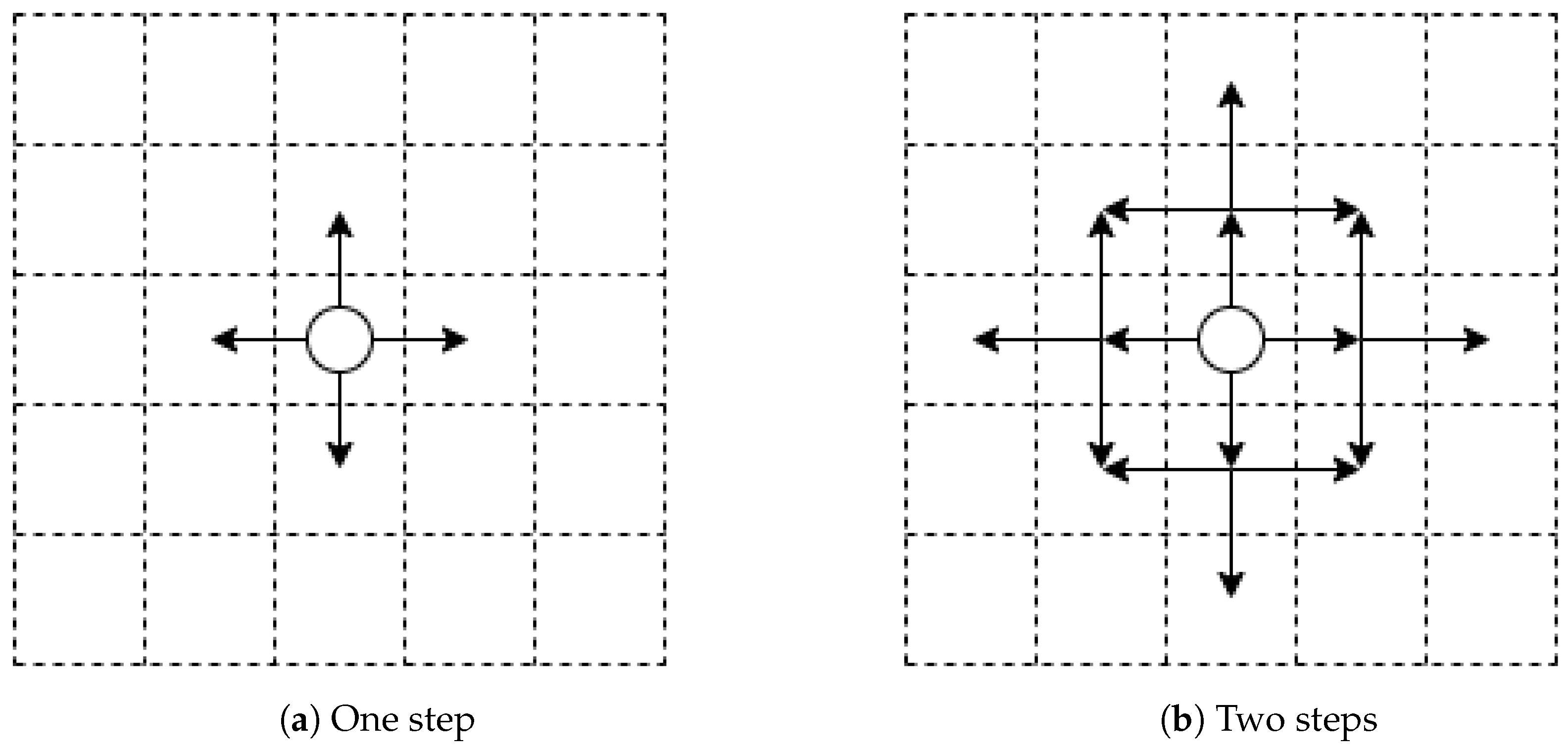
Function of the non-cumulative payment development, depending on the development year, is generally decreasing. Thus, we cannot use the heat equation on a pure triangle. The first approach is to transform the non-cumulative payments triangle before it enters the heat equation. This way appears incorrect, but for the sake of research, we introduce this method, as well. In this case, from each payment, we subtract the median of its column. The resulting triangle is then the initial condition for the heat equation. For every whole row or column of a triangle in time $\tau$ in a form ${\{{\xi }_1,{\xi }_2,\cdots ,{\xi }_{k-1},{\xi }_k\}}^{\tau }$, a vector with boundary conditions will simply be ${\{{\xi }_1,{\xi }_1,{\xi }_2,\cdots ,{\xi }_{k-1},{\xi }_k,{\xi }_k\}}^{\tau }$, ensuring that no heat will enter or leave. (Nota bene: these boundary conditions are in Neumann’s form). To secure stability, we set $dt=0.05$ with $dx=dy=1$ and the number of steps being at least two for letting the heat propagate to at least all eight adjacent cells (see Figure 4b).

For our purposes, we set a maximum number of steps to four. After running the heat equation, it is important to transform the adjusted triangle back to the original form by adding medians to its values. At this point, we can run methods for reserves computation on a new adjusted triangle. In practice, however, an insurance company does not have a stable number of clients during accident years, for instance, which calls for a solution.

2.4.2. Practical Use—Heat Equation Adjustment

Instead of transforming the triangle, we try to transform the heat equation itself to be able to cope with systematic changes during the accident years, as well as the natural decline of payments during the development period. Let us rewrite the Formula (10) to

$$u_{i,j}^{\tau +1}=\frac{dt}{d{x}^2}\left[(u_{i+1,j}^{\tau }-u_{i,j}^{\tau })+(u_{i-1,j}^{\tau }-u_{i,j}^{\tau })\right]+\frac{dt}{d{y}^2}\left[(u_{i,j+1}^{\tau }-u_{i,j}^{\tau })+(u_{i,j-1}^{\tau }-u_{i,j}^{\tau })\right].$$

(12)

We compare incomparable values in all four round brackets. It is similar to comparing today’s 100 € to 100 € in 5 years. Therefore, we simply use the equivalent to the compounding and discounting approach.

Let us define horizontal factors between the non-cumulative values of payments as

$${\widehat{h}}_j=m\left(\left\{\frac{X_{0,j+1}}{X_{0,j}},\cdots ,\frac{X_{I-1,j+1}}{X_{I-1,j}}\right\},\left\{X_{0,j},\cdots ,X_{I-1,j}\right\}\right),$$

(13)

where function $m(x,w)$ is a weighted median of values $x_j$ and of their corresponding weights $w_j$. In case a local horizontal factor $\frac{X_{i,j+1}}{X_{i,j}}$ does not make sense (e.g., division by zero), the weighted median is computed without this local factor and its corresponding weight. We set the horizontal factor to $0.5$ if it does not exist or is lower than zero. As a consequence, we preserve decreasing in the non-cumulative payments during the development period. Whether a constant is to be precisely determined in this case is up to the reader.

The vertical factors are set simply as

$${\widehat{v}}_i=\frac{X_{i+1,0}}{X_{i,0}},$$

(14)

to eliminate possible edge problems during the accident years. $X_{i,0}$ is the first possible non-cumulative payment (development year zero). Weighted medians are not used here because payments up to one year are the biggest carrier of information. In practice, it is not unusual that the outlier in the later development period clearly damages the ratio of payments between the accident years. The vertical factor is set to 1 if it does not exist or is lower than zero. As a result, we assume no systematic change between the following accident years.

For both factors (horizontal and vertical), we set their distance from zero to be at least $0.001$ to avoid unreasonably high multiplications. Then the adjusted step for the numerical solution is set as

$$\begin{array}{c}{u}_{i,j}^{\tau +1}=\frac{dt}{d{x}^2}\left[\left(u_{i+1,j}^{\tau }\frac{1}{\sqrt{v_i}}-u_{i,j}^{\tau }\sqrt{v_i}\right)+\left(u_{i-1,j}^{\tau }\sqrt{v_{i-1}}-u_{i,j}^{\tau }\frac{1}{\sqrt{v_{i-1}}}\right)\right]\hfill \\ \hfill +\frac{dt}{d{y}^2}\left[\left(u_{i,j+1}^{\tau }\frac{1}{\sqrt{h_j}}-u_{i,j}^{\tau }\sqrt{h_j}\right)+\left(u_{i,j-1}^{\tau }\sqrt{h_{j-1}}-u_{i,j}^{\tau }\frac{1}{\sqrt{h_{j-1}}}\right)\right].\end{array}$$

(15)

2.4.3. Non-Positive Increments Estimates

The stochastic modification methods described in Section 2.1.2 are based on the computation of the residuals using the Formula (1). The square root in the denominator implies that the bootstrap method cannot be used when estimated increments are zero or lower (meaning that the development factors must be more than one).

For this case, we use the one-dimensional heat equation to try to adjust the development factors to values greater than one. The initial condition for the row of the triangle $\{r_1,r_2,\cdots ,r_{k-1},r_k$} will be the row itself. The boundary condition in time $\tau$ will be ${\{r_1,r_1,r_2,\cdots ,r_{k-1},r_k,r_k\}}^{\tau }$. The time step is set to $dt=0.05$ to satisfy stability condition (7), having $dx=1$. The maximum number of steps is set to 8. If, after running the heat equation, any development factor is still one or lower than the bootstrap, the methods from Section 2.1.2 will not be used.

3. Results

3.1. Practical Use—Triangle Transformation

Let us start with the triangle with an artificially created outlier, the number with bold in

Table 10. Non-cumulative payments with an artificial outlier.

	0	1	2	3	4
0	27,595,371	16,541,317	955,064	221,151	253,000
1	30,177,361	35,000,000	2,654,823	5200
2	27,421,072	13,715,687	4,783,474
3	22,757,188	12,915,963
4	37,314,432

Source: Adapted from (Gatialova 2010).

.

The original non-outlier value was 15,888,572. After three steps1 of the two-dimensional heat equation, we get the result displayed in

Table 11. Non-cumulative payments triangle after three steps of the heat equation in two dimensions.

	0	1	2	3	4
0	28,296,830	17,912,300	2,003,148	625	254,360
1	31,230,863	26,046,477	4,647,049	162,163
2	27,389,026	16,254,519	4,301,611
3	25,447,541	12,975,899
4	35,388,691

Source: own production.

with reduced outlier value with bold.

For the following results, it is important to be aware of the fact that the reserves were computed using the original vector of earned premium from (Gatialova 2010) for

Table 12. Computed quantiles of reserves with outlier without using the heat equation in two dimensions.

	50th	75th	90th	95th
CL	34,130,722
CC	28,506,180
BCL	34,496,727	47,019,901	64,831,451	80,843,126
BCC	28,868,084	34,393,630	39,639,634	42,741,521
BCL_C	29,435,838	47,904,121	54,952,155	55,865,054

Source: own production.

and

Table 13. Computed quantiles of reserves with outlier using the heat equation in two dimensions.

	50th	75th	90th	95th
CL	31,616,200
CC	28,492,405
BCL	31,560,638	36,415,770	41,173,703	44,909,633
BCC	28,372,479	31,116,043	33,344,732	34,786,776
BCL_C	30,043,105	33,191,035	39,069,138	40,057,328

Source: own production.

.

As expected, besides the slightly modified point estimates, using the heat equation caused lower variance in the bootstrap methods.

3.2. Non-Positive Increments Estimates

Let us take the original triangle from (Gatialova 2010) (

Table 14. Triangle of non-cumulative payments with a negative value above the diagonal.

	0	1	2	3	4
0	27,595,371	16,541,317	955,064	−10,000	253,000
1	30,177,361	15,888,572	2,654,823	5200
2	27,421,072	13,715,687	4,783,474
3	22,757,188	12,915,963
4	37,314,432

Source: Adapted from (Gatialova 2010).

) and set one increment to −10,000. It is up to the reader why $-500$ is not enough in this case.

After running the heat equation in one dimension (apparently on the first row of the triangle), we get the following adjusted triangle (

Table 15. Triangle of non-cumulative payments after the adjustment by the heat equation in one dimension.

	0	1	2	3	4
0	27,042,668	16,314,707	1,686,123	51,403	239,850
1	29,462,922	15,941,324	3,184,029	137,681
2	26,735,803	13,954,346	5,230,085
3	22,265,127	13,408,024
4	37,314,432

Source: own production.

).

Whereas the sum of payments in each row before and after the adjustment is the same. Rounded development factors are summarized in

Table 16. Development factors before and after the adjustment.

	$0\to 1$	$1\to 2$	$2\to 3$	$3\to 4$
Before (Table 14)	1.54711	1.06390	0.99995	1.00561
After (Table 15)	1.56507	1.07802	1.00202	1.00532

Source: own production.

.

As soon as all the development factors are greater than one, the adjusted triangle can be used as an input for the bootstrap method using residuals. For other methods, the original triangle was used. Afterwards, the reserves shown in

Table 17. Computed quantiles of reserves for the Table 14 applying the heat equation in one dimension.

	50th	75th	90th	95th
CL	27,465,613
CC	23,074,551
BCL	30,027,309	34,617,421	39,368,558	42,569,244
BCC	24,681,341	26,913,779	29,159,449	30,773,575
BCL_C	27,663,269	29,795,669	31,530,287	33,215,173

Source: own production.

are obtained.

3.3. Practical Use—Heat Equation Adjustment

Let us introduce a real insurance company example (Motor insurance). As NBS is allowed to publish only aggregated data, the triangle is multiplied by a constant. Numbers are therefore different, but the ratios stay the same. For our purposes, it is also sufficient to show only a part of the triangle as shown in

Table 18. Triangle of non-cumulative payments for Motor insurance.

	0	1	2	3	4	⋯
2002	747,090	179,926	2209	2454	0
2003	1,258,341	675,284	44,707	2134	5332
2004	4,014,851	1 107,703	30,763	2752	−9282
2005	4,594,908	1,291,662	20,091	63,549	−3747
2006	6,560,239	1,567,906	−23,166	9402	14,918
2007	8,578,376	1 991,642	43,927	−16,275	3801
2008	10,200,767	1,698,292	12,573	7004	55,160
2009	9,229,452	1,451,055	28,551	−1621	9922
⋮

Source: NBS—adjusted report.

.

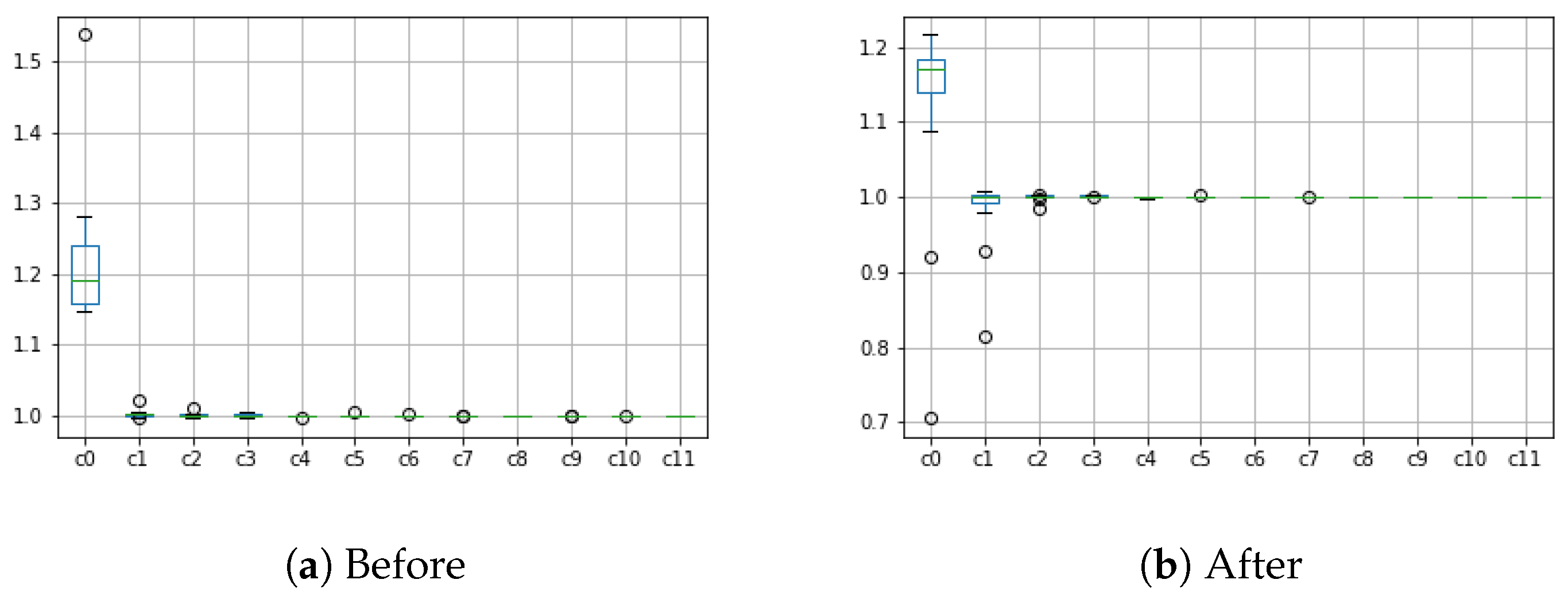
In this case (systematic changes during accident years), it is not appropriate to use the triangle transformation technique. Some outliers can be smoothed; some others will appear. Figure 5 shows boxplots of the local development factors before and after the inappropriate adjustment.

Using the heat equation adjustment technique from the Section 2.4.2, we get the boxplots of the local development factors as shown in Figure 5, where existing outliers are smoothed and the new ones do not appear again as they do in Figure 6.

Both figures represent the boxplots of the local development factors for each development year. The Figure 5 shows how the development factors change after applying the heat equation on the original development triangle using an inappropriate triangle transformation technique. In Figure 6, the appropriate heat equation adjustment technique has been used.

4. Discussion

There are different approaches to mitigate outliers during the loss reserves estimation. The mitigation of outliers is usually dependent on a specific methodology (Bornhuetter and Ferguson 1972; Bühlmann and Straub 1983; Stanard 1985; Taylor 1977; Verdonck et al. 2009) for calculating reserves and the subsequent creation of a robust alternative.

Current research on the removal of outliers in contaminated datasets for claims reserves is quite limited as the traditional methods are preferably applied. In the light of the most recent works published in this topic (Avanzi et al. 2022b; Badounas et al. 2022), our method takes on a different approach. First, outlying values are detected and smoothed by the heat equation application. The resulting development triangle could then be used as an input for any method without the need for its robustification.

The future work shall address the appropriate setting for the parameters of the numerical solution of the heat equation, such as the step length or the maximum number of steps. The current parameters are set as constants, which seems to be sufficient for the demonstration of the methodology.

5. Conclusions

Outlier management in the non-life development triangles for calculation of technical reserves estimates has been thoroughly addressed in the existing literature. This article presents another way to approach the problem naturally occurring in the non-life development triangles. The heat equation and its properties introduced in the paper help address the lack of person-specific data while keeping the whole original triangle payments total sum and reasonable differences between the original and the backward estimated triangle. The method enables to smooth out the outliers across the neighboring years instead of their elimination which yields more realistic results. Hence, the unscaled Pearson’s residuals for the stochastic modifications and the one-dimensional heat equation are used to adjust the development factors to values greater than one. Otherwise, the bootstrap method cannot be used. Introducing the one-dimension and the two-dimension heat equation offers an uncommon overview of the simplest stochastic process coupled with the physical equation and their potential in overcoming the challenges of the field.

References

1. Avanzi, Benjamin, Mark Lavendera, Greg Taylora, and Bernard Wong. 2016. On the impact, detection and treatment of outliers in robust loss reserving. Paper presented at the Actuaries Institute 2016 General Insurance Seminar, Melbourne, Australia, November 13–15. [Google Scholar]
2. Avanzi, Benjamin, Mark Lavender, Greg Taylor, and Bernard Wong. 2022a. Detection and treatment of outliers for multivariate robust loss reserving. arXiv arXiv:2203.03874. [Google Scholar]
3. Avanzi, Benjamin, Mark Lavender, Greg Taylor, and Bernard Wong. 2022b. On the impact of outliers in loss reserving. arXiv arXiv:2203.00184. [Google Scholar]
4. Badounas, Ioannis, Apostolos Bozikas, and Georgios Pitselis. 2022. A robust random coefficient regression representation of the chain-ladder method. Annals of Actuarial Science 16: 151–82. [Google Scholar] [CrossRef]
5. Badounas, Ioannis, and Georgios Pitselis. 2020. Loss reserving estimation with correlated run-off triangles in a quantile longitudinal model. Risks 8: 14. [Google Scholar] [CrossRef]
6. Barlak, Jan. 2021. Stochastické vývojové trojuholníky a ich využitie pri odhadovaní technických rezerv v neživotnom poistení. Available online: https://opac.crzp.sk/?fn=detailBiblioForm&sid=AF3291F10EFAAB2E0DB4B36C36BB&seo=CRZP-detail-kniha (accessed on 23 May 2022).
7. Black, Michael J., and Guillermo Sapiro. 1999. Edges as outliers: Anisotropic smoothing using local image statistics. In Scale-Space Theories in Computer Vision. Berlin/Heidelberg: Springer, pp. 259–70. [Google Scholar] [CrossRef]
8. Bornhuetter, Ronald L., and Ronald E. Ferguson. 1972. The actuary and ibnr. Proceedings of the Casualty Actuarial Society 59: 181–95. [Google Scholar]
9. Brazauskas, Vytaras, Bruce L. Jones, and Ricardas Zitikis. 2009. Robust fitting of claim severity distributions and the method of trimmed moments. Journal of Statistical Planning And Inference 139: 2028–43. [Google Scholar] [CrossRef]
10. Buades, Antoni, Bartomeu Coll, and Jean-Michel Morel. 2006. Image enhancement by non-local reverse heat equation. Preprint CMLA 22: 2006. [Google Scholar]
11. Bühlmann, Hans. 2016. Historical origin of the cape cod claims reserving method. SSRN Electronic Journal. [Google Scholar] [CrossRef]
12. Bühlmann, Hans, and Erwin Straub. 1983. Estimation of ibnr reserves by the methods chain ladder, cape cod and complementary loss ratio. International Summer School. Unpublished. [Google Scholar]
13. Cannon, John Rozier, and Felix E. Browder. 1984. The One-Dimensional Heat Equation. Encyclopedia of Mathematics and Its Applications. Cambridge: Cambridge University Press. [Google Scholar]
14. Cowell, Robert. 2009. Exploration of a Novel Bootstrap Technique Forestimating the Distribution of Outstanding Claimsreserves in General Insurance. Technical Report. London: Faculty of Actuarial Science and Insurance, Cass Business School, City University London. [Google Scholar]
15. Dahms, Rene. 2021. Stochastic Reserving Lecture. Available online: https://ethz.ch/content/dam/ethz/special-interest/math/risklab-dam/documents/Lectures/Stochastic_Reserving_2019.pdf (accessed on 23 May 2022).
16. El Badia, Abdellatif, and Tuong Ha-Duong. 2002. On an inverse source problem for the heat equation application to a pollution detection problem. Journal of Inverse and Ill-Posed Problems 10: 585–99. [Google Scholar] [CrossRef]
17. Embrechts, Paul, and Mario V. Wüthrich. 2022. Recent challenges in actuarial science. Annual Review of Statistics and Its Application 9: 119–40. [Google Scholar] [CrossRef]
18. England, Peter, and Richard Verrall. 1999. Analytic and bootstrap estimates of prediction errors in claims reserving. Insurance: Mathematics and Economics 25: 281–93. [Google Scholar] [CrossRef]
19. Gatialova, Jaroslava. 2010. Rezervy-ich výpočet a význam v životnom a neživotnom poistení. Available online: https://opac.crzp.sk/?fn=detailBiblioForm&sid=5B91E22B52137C4AAB32540D0767 (accessed on 23 May 2022).
20. Gluck, Spencer M. 1997. Balancing development and trend in loss reserve analysis. Proceedings of the Casualty Actuarial Society 84: 482–532. [Google Scholar]
21. Gorguis, Alice, and Wai Kit Benny Chan. 2008. Heat equation and its comparative solutions. Computers & Mathematics with Applications 55: 2973–80. [Google Scholar] [CrossRef]
22. Gurevich, Svetlana. 2016. Numerical Methods for Complex Systems I. Available online: https://www.uni-muenster.de/imperia/md/content/physik_tp/lectures/ws2016-2017/num_methods_i/heat.pdf (accessed on 23 May 2022).
23. Hill, Christian. 2016. Learning Scientific Programming with Python. Available online: https://scipython.com/book/chapter-7-matplotlib/examples/the-two-dimensional-diffusion-equation/ (accessed on 23 May 2022).
24. Itkin, Andrey, Alexander Lipton, and Dmitry Muravey. 2021. Multilayer heat equations: Application to finance. arXiv arXiv:2102.08338. [Google Scholar]
25. Korn, Uri. 2016. An extension to the cape cod method with credibility weighted smoothing. In CAS E-Forum, Summer. Available online: https://www.casact.org/sites/default/files/database/forum_16sforum_korn.pdf (accessed on 23 May 2022).
26. Liu, Huijuan, and Richard J. Verrall. 2010. Bootstrap estimation of the predictive distributions of reserves using paid and incurred claims. Variance 4: 121–35. [Google Scholar]
27. Lowe, Julian. 1994. A practical guide to measuring reserve variability using: Bootstrapping, operational time and a distribution free approach. In Proceedings of the 1994 General Insurance Convention. London: Institute and Faculty of Actuaries. [Google Scholar]
28. Maciak, Matúš, Ivan Mizera, and Michal Pešta. 2022. Functional profile techniques for claims reserving. ASTIN Bulletin 52: 449–82. [Google Scholar] [CrossRef]
29. Mack, Thomas. 1993. Distribution-free calculation of the standard error of chain ladder reserve estimates. ASTIN Bulletin: The Journal of the IAA 23: 213–25. [Google Scholar] [CrossRef]
30. Manolache, Aurora Elena Dina. 2019. Chain claims reserving methods in non-life insurance. Proceedings of the International Conference on Applied Statistics 1: 216–25. [Google Scholar] [CrossRef]
31. Murphy, Daniel M. 1994. Unbiased Loss Development Factors. Available online: https://www.casact.org/sites/default/files/database/forum_94spforum_94spf183.pdf (accessed on 23 May 2022).
32. Peremans, Kris, Pieter Segaert, Stefan Van Aelst, and Tim Verdonck. 2017. Robust bootstrap procedures for the chain-ladder method. Scandinavian Actuarial Journal 2017: 870–97. [Google Scholar] [CrossRef]
33. Peters, Gareth W., Alice X. D. Dong, and Robert Kohn. 2014. A copula based Bayesian approach for paid–incurred claims models for non-life insurance reserving. Insurance: Mathematics and Economics 59: 258–78. [Google Scholar] [CrossRef]
34. Peremans, Kris, Stefan Van Aelst, and Tim Verdonck. 2018. A robust general multivariate chain ladder method. Risks 6: 108. [Google Scholar] [CrossRef]
35. Pesta, Michal. 2011. Bootstrap Methods in Reserving. Available online: https://www2.karlin.mff.cuni.cz/~pesta/NMFM401/pesta-seminar111209.pdf (accessed on 23 May 2022).
36. Saluz, Annina. 2015. Prediction uncertainties in the cape cod reserving method. Annals of Actuarial Science 9: 239–63. [Google Scholar] [CrossRef]
37. Schönlieb, Carola-Bibiane. 2012. Applying Modern Pde Techniques to Digital Image Restoration. Available online: https://www.mathworks.com/company/newsletters/articles/applying-modern-pde-techniques-to-digital-image-restoration.html (accessed on 23 May 2022).
38. Silvestre, Luis. n.d. Heat Equation Solver. Available online: https://www.math.uchicago.edu/~luis/pde/heat.html (accessed on 23 May 2022).
39. Stanard, James N. 1985. A simulation test of prediction errors of loss reserve estimation techniques. Proceedings of the Casualty Actuarial Society 72: 124–48. [Google Scholar]
40. Struzzieri, Paul J., Paul R. Hussian, and Two Pennsylvania Plaza. 1998. Using best practices to determine a best reserve estimate. CAS Forum 10121: 353–413. [Google Scholar]
41. Taylor, Greg C. 1977. Separation of inflation and other effects from the distribution of non-life insurance claim delays. ASTIN Bulletin: The Journal of the IAA 9: 219–30. [Google Scholar] [CrossRef]
42. Verdonck, Tim, and Michiel Debruyne. 2011. The influence of individual claims on the chain-ladder estimates: Analysis and diagnostic tool. Insurance: Mathematics and Economics 48: 85–98. [Google Scholar] [CrossRef]
43. Verdonck, Tim, and Martine Van Wouwe. 2011. Detection and correction of outliers in the bivariate chain–ladder method. Insurance: Mathematics and Economics 49: 188–93. [Google Scholar] [CrossRef]
44. Verdonck, Tim, Martine Van Wouwe, and Jan Dhaene. 2009. A robustification of the chain-ladder method. North American Actuarial Journal 13: 280–98. [Google Scholar] [CrossRef] [Green Version]
45. Widder, David Vernon. 1976. The Heat Equation. Pure and Applied Mathematics. Amsterdam: Elsevier Science. [Google Scholar]
46. Wuthrich, Mario V. 2017. Neural networks applied to chain-ladder reserving. SSRN Electronic Journal. [Google Scholar] [CrossRef]
47. Zaçaj, Oriana, Endri Raço, Kleida Haxhi, Etleva Llagami, and Kostaq Hila. 2022. Bootstrap methods for claims reserving: R language approach. WSEAS Transactions on Mathematics 21: 252–59. [Google Scholar] [CrossRef]
Figure 1. Heat distribution in a rod during the time period.
Risks 10 00171 g001
Figure 2. Escaping heat. Inspired by (Hill 2016).
Risks 10 00171 g002
Figure 3. Damaged image restoration. Source: (Schönlieb 2012).
Risks 10 00171 g003
Figure 4. Heat diffusion to adjacent points.
Risks 10 00171 g004
Figure 5. Failed attempt to outlier elimination using the triangle adjustment technique.
Risks 10 00171 g005
Figure 6. Outlier elimination using the heat equation adjustment technique.
Risks 10 00171 g006