Article

Factors Driving Duration to Cross-Selling in Non-Life Insurance: New Empirical Evidence from Switzerland

1
Center of Data Analysis, Visualisation and Simulation, University of Applied Sciences of the Grisons, Ringstrasse 34, 7000 Chur, Switzerland
2
Department of Actuarial Science, Faculty of Business and Economics (HEC Lausanne), University of Lausanne, Chamberonne—Extranef, 1015 Lausanne, Switzerland
3
Swiss Finance Institute, University of Lausanne, 1015 Lausanne, Switzerland
*
Author to whom correspondence should be addressed.
Risks 2022, 10(10), 187; https://doi.org/10.3390/risks10100187
Submission received: 26 August 2022 / Revised: 14 September 2022 / Accepted: 16 September 2022 / Published: 27 September 2022
(This article belongs to the Special Issue Risks: Feature Papers 2022)

Abstract

:
Customer relationship management and marketing analytics have become critical for non-life insurers operating in highly competitive markets. As it is easier to develop an existing customer than to acquire a new one, cross-selling and retention are key activities. In this research, we focus on both car and household-liability insurance products and consider the time a customer owning only a single product takes before buying the other product at the same insurer. Based on longitudinal consumer data from a Swiss insurance company covering the period from 2011 to 2015, we aim to study the factors driving the duration to cross-selling. Given the different dynamics observed in both products, we separately study the car and household-liability insurance customer cohorts. Considering the framework of survival analysis, we provide descriptive statistics and Kaplan–Meier estimates along major customer characteristics, contract history and distribution channel usage. For the econometric analysis of the duration, we compare the results from Cox and accelerated failure time models. We are able to characterize the times related to the buying behavior for both products through several covariates. Our results indicate that the policyholder age, the place of residence, the contract premium, the number of contracts held, and the initial access channel used for contracting influence the duration to cross-selling. In particular, our results underline the importance of the tied agent channel and the differences along the geographic region and the urbanicity of the place of residence. By quantifying the effects of the above factors, we extend the understanding of customer behavior and provide a basis for developing models to time marketing actions in insurance companies.

1. Introduction

One of the main objectives of insurance companies targets profitable growth, while the evaluation of adequate premium levels by actuaries and proper risk selection by underwriters is key for keeping profitability, the marketing departments and their customer relationship management (CRM) is concerned about attracting new customers (Bieck et al. 2010; Maas et al. 2008). Growing in saturated markets is difficult and customers tend to be less loyal when competition is intense (Guillen et al. 2008). Like for many convenience products, customers tend to seek for the lowest priced offers leading to increasingly important fluctuations in insurance portfolios (Kamakura et al. 2003). In many markets, if an insurer acquires a new customer, a competitor loses one (Kamakura 2007; Prinzie and Van den Poel 2006). Since serving an existing customer is more cost effective than acquiring a new one (Fornell and Wernerfelt 1987), insurers try to retain their customers and to strengthen long-term relationships (Gupta et al. 2006). For example, Dutang (2012) shows that cross-selling has a preventive effect on lapse in property and casualty insurance. In this context, several streams of research have developed, analyzing the factors driving the customer journey (see, e.g., Staudt and Wagner 2018) and studying the next purchases (see, e.g., Mau et al. 2015, 2017, 2018). Cross-selling, i.e., selling additional items unrelated to a previous purchase, is one of the main CRM tools to forge relationships (Prinzie and Van den Poel 2006; Verhoef and Donkers 2005). Such strategies gain in importance especially when competition is strong (Prinzie and Van den Poel 2007). Since companies have only limited resources, it is important to identify the personal incentives that lead customers to cross-buy, respectively, to identify the moment when pushing cross-selling is most effective. Nowadays, many service transactions are automatized by technology and it is important to integrate the drivers of cross-buying behavior (Knott et al. 2002; Kumar et al. 2008). Moreover, given that an overly aggressive cross-selling strategy can weaken the customer relationship, cross-selling must be applied carefully, targeting the right customer with the right product at the right time. This is only possible if the prevalent buying and successful selling patterns are well understood. The first product bought and the elapsed time to the next purchase can explain part of the customer behavior dynamics (Jain and Vilcassim 1991) and help to time marketing actions (Grewal et al. 2004). Research by Ngobo (2004); Verhoef and Donkers (2005); Verhoef et al. (2001) among others has been conducted to statistically describe and determine the factors influencing cross-buying in non-life insurance. However, to the best of our knowledge, little research has been interested in analyzing the time a policyholder takes to cross-buy, i.e., the inter-purchase time between products, and no research has been done relating that duration to the policy attributes.
In this paper, we consider the two most common non-life insurance products, car and household-liability insurance. We are interested in the time a customer owning only a single product takes before contracting the other product at the same insurer. Thus, we concentrate on two transitions from the car, respectively, household-liability insurance single-product state to the state of owning both products. Based on the framework of survival analysis, we aim to evaluate two duration models to identify and quantify the effects of selected factors that significantly relate to the time taken for cross-selling. The objective is to compare the results of the traditionally used Cox model with the one of an accelerated failure time model by extending their use for continuous variables in a non linear way. We calibrate our models using longitudinal client data from a top-tier Swiss insurance company covering the period from 2011 to 2015. Available covariates include customer attributes (age, urbanicity of the residence and geographic region), product attributes (premium, number of damages, other contracts held) as well as the first purchase channel. We base our analysis on 60,752 customers having contracted their first car ( 28,388 ) or household-liability ( 32,364 ) insurance product in 2011.
When referring to survival analysis, the “survival” time corresponds to the inter-purchase time between the single- and two-products states. The traditional “survival probability” relates to the probability of remaining a single-product customer. Through the period covered by our data, we observe some customers buying the second product and allowing the calculation of the survival time. At the end of the period not all customers have transited. This is related to the fact that a customer may never buy the second product, e.g., because not owning a car or living with a partner that has taken out insurance, that the other contract is taken with a competitor or that the observation frame is too short. In order to integrate this right-censoring in our statistics, we use Kaplan–Meier estimates to describe the durations. For the econometric modeling, we propose to apply Cox and accelerated failure time (AFT) models, while Cox models are typically used for such study (Ansell et al. 2007; Prinzie and Van den Poel 2006), we compare our results with AFT models that provide a direct relationship between the explanatory variables and the duration (see, e.g., Fuino and Wagner 2020; Kalbfleisch and Prentice 2002). Studies in the marketing literature primarily use demographic and economic variables as risk factors (Grewal et al. 2004). We use the covariates contained in our data, i.e., include customer information recorded at contract inception, to identify customers with similar buying dynamics (see also Frees 2015; Laas et al. 2016). The Cox and AFT models are linear models, i.e., the factors are included as linear predictors. Since this assumption can be too restrictive for continuous variables like the customers’ age or the premium levels (Denuit and Lang 2004; James et al. 2013), they are traditionally segmented into categories, often unrelated to the data (Dougherty et al. 1995; Ohlsson and Johansson 2010). In this context, we apply a data-driven method to bin the continuous variables (Henckaerts et al. 2018; Staudt and Wagner 2019). The method is based on smoothing functions describing the effects of the continuous variables. The Cox model can be extended to such functions by transforming it into a Poisson generalized linear model (Wood 2017). Data-driven categories are built by applying evolutionary trees (Grubinger et al. 2014), a machine learning method, on the effects of the smoothing functions, leading to a model with only categorical variables. Such model may be useful for the management to determine groups particularly susceptible for cross-buying and to define actions and incentives.
We find that customers with a household-liability insurance contract show different times to cross-selling than the ones with a car insurance contract: the probability of the latter buying household-liability insurance increases more importantly after about two years of customer relationship and reaches about 20% of the initial cohort after five years. Our econometric study shows that the place of residence, the number of contracts held, the access channel, the age and the premiums of the contracts held are relevant factors that significantly relate to the duration to cross-selling. Thereby, our numerical results support, among others, the relevance of the tied agent channel, the differences along geographic regions and the importance of the urbanicity of the place of residence.
The remainder of the work is structured as follows: In Section 2, we outline the states, transitions and the data, introduce the notations used in the sequel and statistically describe the inter-purchase time and the explanatory variables. In Section 3, we measure the relation of the available covariates on the duration to cross-selling. For both car and household-liability cohorts, we derive optimal econometric Cox and AFT models and compare the results with the observations made from the descriptive statistics. We conclude in Section 4.

2. Insurance Portfolio Data and Cross-Selling Statistics

Our analysis relies on a longitudinal dataset of a Swiss insurer comprising all new customers that have contracted a car or a household-liability insurance product in the year 2011. These policyholders are observed over a period of five years, i.e., until 2015. We are interested in studying the time it takes them to buy the other product, i.e., car insurance for a household-liability insurance single-product costumer or household-liability insurance for a car insurance single-product customer. In Section 2.1, we describe the considered transitions and provide statistics on the portfolio development, cross-selling probabilities and goodness-of-fit statistics for the inter-purchase times. In Section 2.2, we detail the available variables in the data, illustrate the relative frequencies along the characteristics of the observations and provide descriptive statistics on the duration along the covariates.

2.1. Time to Cross-Selling

As laid out in the Introduction, we focus in our analysis on the two main non-life insurance products for private customers. We consider customers having bought a car (CA) or household-liability (HL) insurance product in 2011. We do not distinguish between different modules and deductible levels of the insurance cover bought, e.g., motor third party liability, collision and parking damage in CA and the components of household and liability insurance in HL, while motor third party liability, one module of CA insurance, is compulsory, components of HL insurance are not in Switzerland. Customers can freely choose their insurance provider from more than ten sizable players. A customer is recorded in our data if he or she has underwritten a CA or HL contract with the insurer providing the data, otherwise the customer relationship is not observed. We consider that a policyholder has done cross-buying if he or she holds a combination of both products CA and HL denoted by “CA & HL”. In Figure 1, we illustrate both transitions we are interested in. The transitions originate with customers holding CA or HL insurance as starting state. In practice, different scenarios for cross-buying exist: either a customer is buying the additional product for the first time, e.g., when buying a car or a young customer establishing an own household, or a customer is coming from a competitor.

2.1.1. Portfolio Development

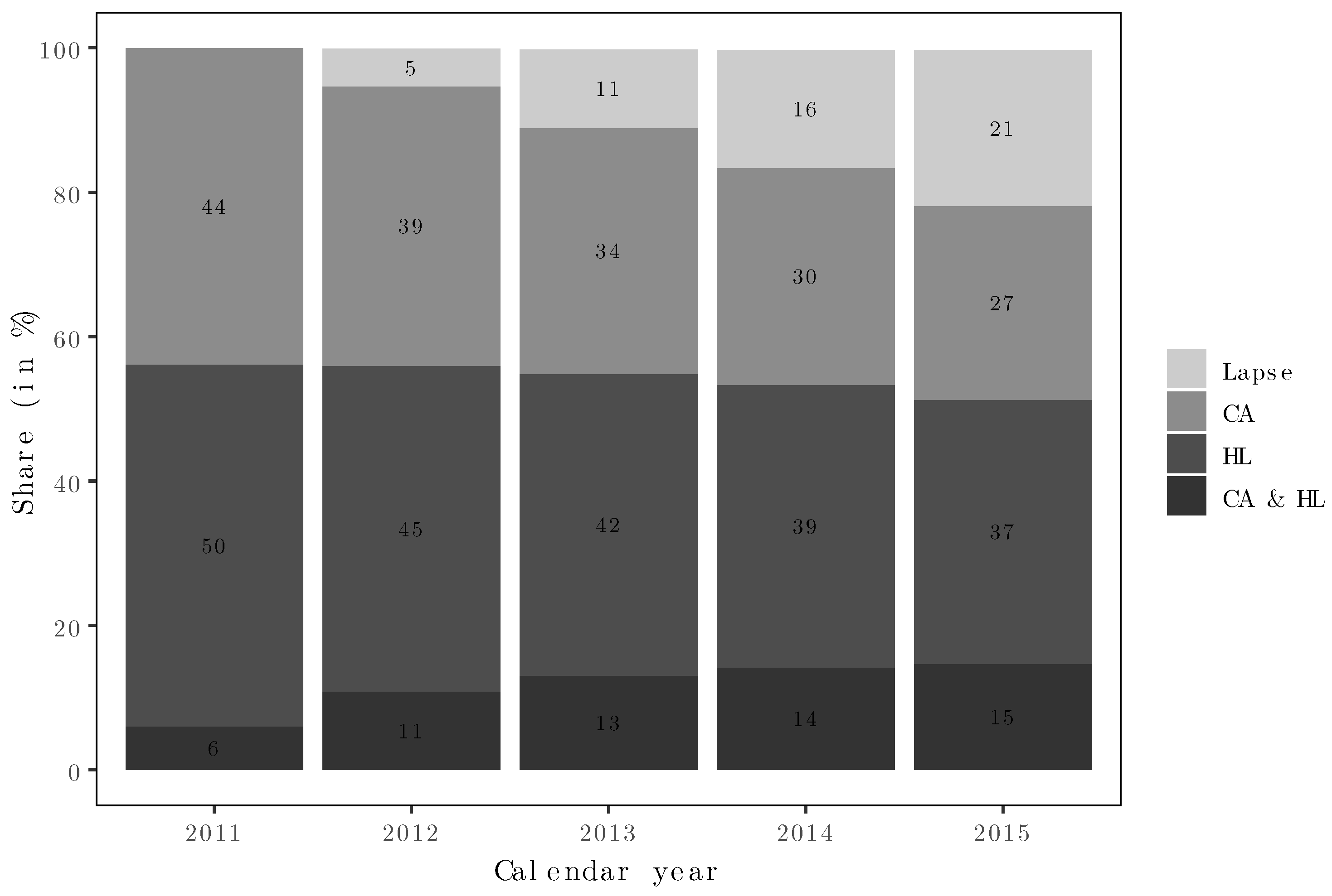
In Figure 2, we illustrate the aggregated development of the portfolio through the years from 2011 to 2015. The first bar represents the original state where 100% corresponds to the 60,752 customers recorded at the end of the year. We observe a higher share of HL single-product customers (50%) when compared to CA (44%). Further 6% of the customers have underwritten both CA and HL in the first year. This share of two-products customers (CA & HL) is increasing to 15 % in 2015. At the same time, we also observe contract cancellations: the share of lapsing customers yields 22% in 2015, while HL customers represent half of the portfolio in 2011, they still are 37 % in 2015. The share of CA policyholders decreases faster, from 44% in 2011 to 27% in 2015. Customers who cancel their contracts are not further analyzed in this paper; such analysis can, for example, be found in Staudt and Wagner (2018).

2.1.2. Duration to Cross-Selling and Right-Censoring

We are interested in the time it takes to perform the transition after buying the first CA or HL insurance product. It has to be noted that, given our observation period of five years, records will be right-censored. In fact, some customers may not need and thus not buy the other product, some may have an existing second contract with a competitor or buy the other product at a competitor. Sometimes contract terms foresee long cancellation and thus waiting periods so that our five-years period is too short to observe further dynamics of customers changing their providers. Furthermore, we note that we cannot observe cross-buying behavior if the customer underwrites the second product at a competitor. The inter-purchase time will depend on various factors. We study some of them through the available recorded covariates in our data (see Section 2.2). Nevertheless, we acknowledge that the generalization of our results is limited by the fact that records stem from one single insurer and the observed dynamics are subject to the underlying unobserved strategy of the insurer, e.g., regarding particular efforts in cross-selling and specific marketing actions. We cannot control for such actions in our study and must keep aware of the related potential bias. Finally, in our data, policyholders may hold other insurance contracts at inception, including other non-life insurance products like travel insurance or life insurance policies. We consider the presence of such contracts. In the following, for simplifying the writing, we call CA and HL customers or “cohorts” the set of customers having contracted CA, respectively, HL insurance in 2011.
Our records exhibit a total of 60,752 customers in the CA and HL cohorts. We count 28,388 CA customers and 32,364 HL contracts. Given that the inception date of the relationship with the CA or HL product is known, we do not have to deal with left censoring. For the first and, if applicable, for the second contract the exact underwriting dates are recorded so that we calculate the inter-purchase time T in days. All observations where the customer has not bought the second product by the end of the observation period are right-censored and marked accordingly with a binary variable (Jackson 2016; Kalbfleisch and Prentice 2002; Moore 2016). In our case, right-censoring is uninformative as the reasons why cross-selling has not taken place are unrelated to the outcome. The share of right-censoring is lower in the case of the CA cohort with 81% remaining single-product customers after five years. This share is 83% for the HL cohort.

2.1.3. Kaplan–Meier Estimates for the Cross-Selling Probability

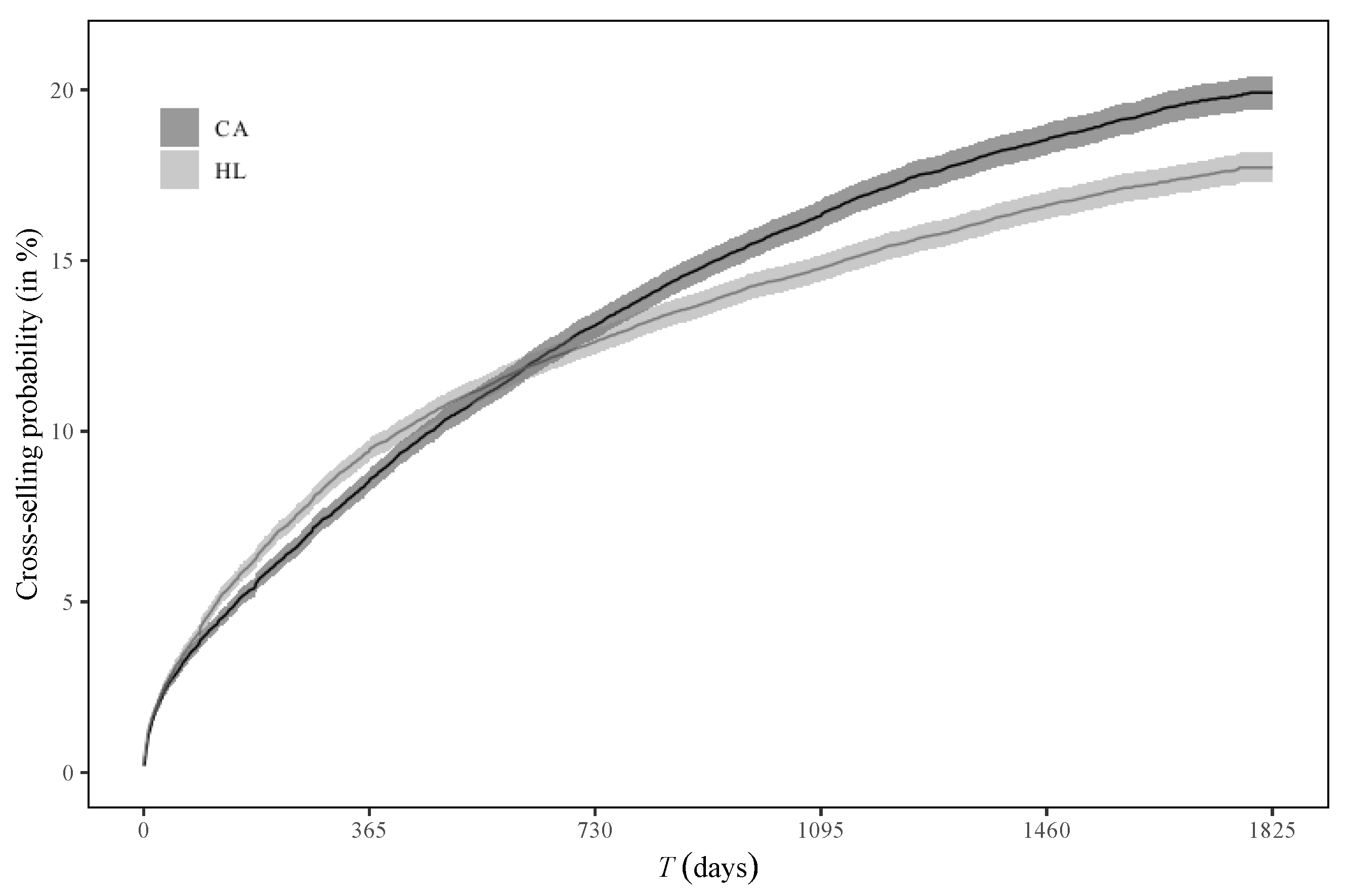
In the following, we consider the time to cross-selling for both products. For this purpose, we are interested in the cross-selling probability. This can be derived from the traditional Kaplan–Meier (KM) estimator in survival analysis. In fact, the probability of cross-selling is the complementary probability, 1 P ( KM ) , to the probability P ( KM ) of remaining a single-product customer (“survivor”). In Figure 3, we report the cross-selling probability for both CA and HL cohorts. We indicate the 95% confidence intervals (gray shaded area), while the differences between both cohorts are minor during the first year, we clearly observe a higher probability for CA customers to buy HL insurance after two years. This is in line with the overall observation in Figure 2 where a larger share of HL customers remains in the single-product state. The differences between both cohorts’ inter-purchase times can be confirmed statistically by the log-rank test (p-value smaller than 0.01, (Aalen et al. 2008)). Following this observation, we study both CA and HL cohorts separately in the sequel.

2.2. Covariates and Descriptive Statistics

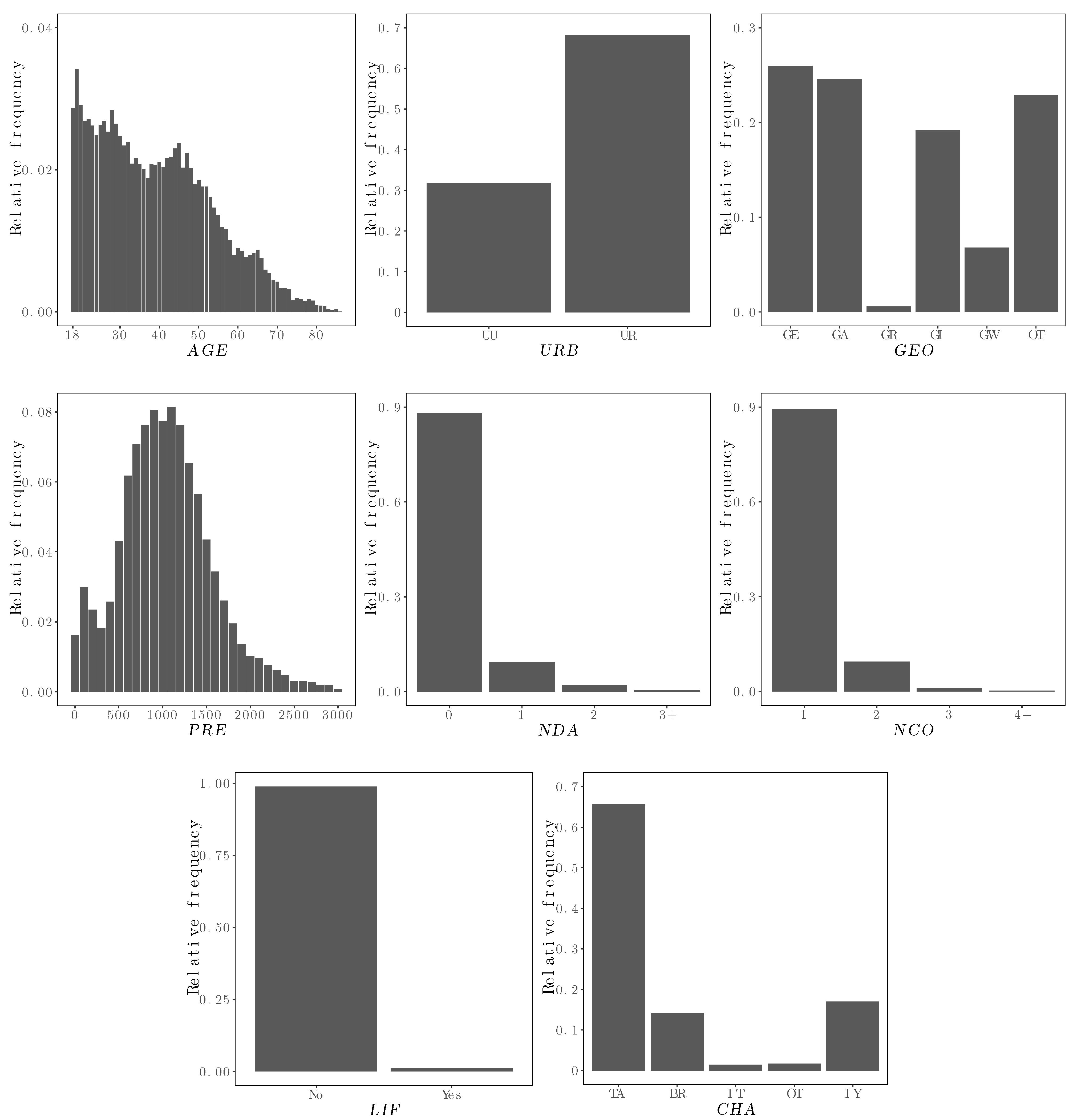
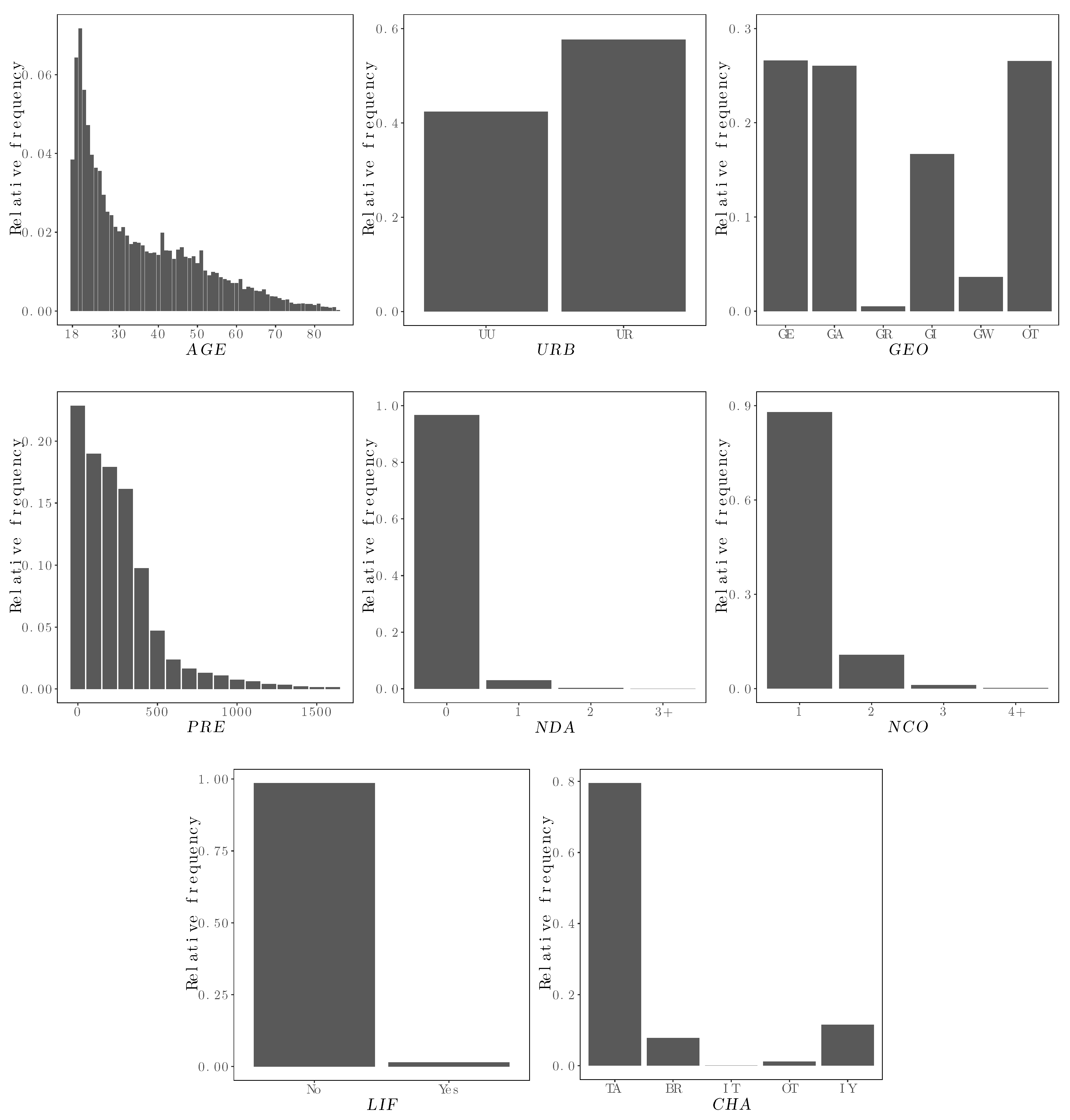
Our data include comprehensive information on the customers, their contracts and the channel used for buying their first CA or HL policy. In Table 1, we summarize the available explanatory variables contained in the dataset. They reflect the information the insurer gathers at contract inception. The data about the policyholders include their age A G E as well as the urbanicity U R B , urban or rural, and the geographic region GEO linked to their place of residence. The geographic region variable consists of five main regions in Switzerland (Lüdi and Werlen 2005) and one categorical value for customers outside of Switzerland (OT). The five Swiss regions that we consider are the East and West Swiss Plateau (GE and GW), the Alps and Prealps (GA), the Romandy (GR) and the Italian-speaking area of Switzerland (GI).1 The products CA and HL are described through the contract premium P R E 2 paid by the policyholders and the number of damages declared to the insurer. The variable NDA specifies four categories of having either no claim (0), one (1), two (2), or three and more ( 3 + ) claims. The number of contracts NCO variable counts the total number of policies a customer holds at CA or HL contract inception. Thereby, each product line is counted once along, e.g., travel, legal protection and life insurance. NCO contains four categories of having underwritten either one (1), two (2), three (3) or four and more ( 4 + ) contracts. The binary variable L I F specifically indicates if the customer has a life insurance contract. The interaction channel used by the policyholder to buy the CA or HL product is given through the access channel variable CHA . The latter records if buying from either a tied agent (TA), an independent intermediary (IY), a broker (BR), the Internet/insurer’s website (IT) or another channel (OT, e.g., by telephone or via particular types of brokers). Tied agents represent the most important part of the sales force at Swiss insurers and they are exclusively linked to the insurer while brokers BR are not. We graphically illustrate the relative frequencies of observations in both CA and HL cohorts along the above variables in Figure 4 and Figure 5.
In the following, we describe the inter-purchase time quantiles in both CA and HL cohorts. In Table 2, we report the relative shares of observations contained in our data as well as the T 5 % , T 10 % and T 15 % time quantiles. The quantiles correspond to the time needed for 5%, 10%, respectively, 15%, of the customers to buy the other product. The values are derived from the KM estimates determined for each of the explanatory variables and categories. The quantiles are measured in days and can only be calculated if at least 5%, 10% or 15% of the customers have been observed cross-buying. In fact, given the high prevalence of right-censoring in our data, these cross-selling shares are not reached along all attributes. In such cases, we state the value as “n.a.” standing for not applicable. For the continuous variable age of the policyholder we consider four age classes commonly found in insurance companies, namely, 18–25, 26–40, 41–65 and 66+ years. For the contract premium, we determine four classes, separately for both cohorts, using the rounded quartiles (25%, 50% and 75%) as limits.3 The values can be found in the first column of Table 2.
The inter-purchase time quantiles related to the CA cohort are reported in the first (left) part of Table 2. Policyholders aged from 41 to 65 years represent the largest group and have the highest T 5 % = 250 and T 10 % = 781 quantiles. This means that it takes 250, respectively, 781, days to cross-sell the HL product to 5%, respectively, 10%, of the CA product holders. Young customers aged from 18 to 25 years (share of 22.3%) have cross-selling times that are four times lower with 15% of them buying the HL product after 349 days ( T 15 % = 349 ). In fact, considering their life cycle, younger customers have more changing needs, e.g., due to new family circumstances and own acquisitions. New CA policyholders aged 66 years or older represent only 5.1 % of the data. This is related to the fact that at higher ages less customers need a new insurance or change their provider (Eling and Kiesenbauer 2014; Staudt and Wagner 2018). Nevertheless, some of them cross-buy in a rather short interval ( T 5 % = 25 ). Most customers observed in the portfolio are living in a rural region ( 68.3 % ) and have much shorter durations to cross-selling. Throughout the geographic regions we also observe important heterogeneity: The East Swiss Plateau ( 26 % ) has a 10%-inter-purchase time quantile of 509 days. The same quantile, in one of the smallest regions, the Italian-speaking area of Switzerland ( 6.8 % ), yields T 10 % = 1223 days while in the Alps and Prealps ( 24.6 % ) and the West Swiss Plateau we observe T 10 % = 365 , respectively, 380 days. With regard to the contract premiums, we observe that customers paying a car premium P R E CA below CHF 747 take much longer before buying a HL product when compared to those with larger contracts. Expectedly, most customers (88%) have no declared damages (see, e.g., Denuit and Lang 2004; Klein et al. 2014; Ohlsson and Johansson 2010). We note that the more damages a customer has declared, the faster he or she cross-buys. In fact, each report of a damage gives an opportunity for the insurer to interact with the customer beyond the settlement of the claim. The fact that claims promote cross-selling activities is in line with previous findings by, e.g., Kamakura (2007). The vast majority of policyholders ( 89.3 % ) have only one contract at inception. Customers with more contracts are cross-buying faster, which can be explained by the tighter relationship and higher frequency of interaction with the insurer (Verhoef et al. 2001). Nevertheless, some of these observations need to be taken with care since the very short durations may be linked to multiple contracts underwritten at the same time but appearing with a delay in the records. Having a life insurance product considerably reduces the cross-selling times. The most popular sales channel in Switzerland is the tied agent channel. For insurers, tied agents are important for cross-selling leading to shorter production times when compared to the other channels. After one year (365 days), 10% of tied agents’ CA customers have also contracted a HL product. This is also true for the internet channel. Although, the internet channel at the studied insurer allows only single-product purchases, the strategy of the insurer asks tied agents to contact online customers and follow up closely with them after their initial online purchase to promote cross-selling. In line with the results of Staudt and Wagner (2018), brokers have a negative influence on cross-buying since independent brokers propose the most adequate product from any company to their customers and do not give a particular weight to earlier purchases at a given firm. Correspondingly, cross-selling times in that group are about five times longer with, e.g., T 5 % = 524 and T 10 % = 1676 .
We provide the duration to cross-selling time quantiles for the HL cohort in the second part of Table 2. Customers from the youngest age group are most numerous ( 38.9 % ) and present the shortest time with T 15 % = 919 days to reach the 15% cross-selling threshold. As found in the statistics for CA, HL customers living in a rural region ( 57.7 % ) have importantly smaller durations to cross-selling with 10% having a CA contract already after 289 days. This is to be compared with urban customers where 849 days are required to reach the same level. Policyholders paying a contract premium between CHF 110 and 252 are the slowest cross-buyers when compared to the other groups. In the HL cohort, 96.7% of the policyholders have not reported any damages. To interpret the effect of the number of damages on the cross-selling times in the remaining small population, an econometric study under consideration of significance levels is necessary. We observe that the HL cohort contains about 88 % single-product customers and 98.6 % have no life insurance contract. As for the CA cohort, the tied agent is the major access point for HL ( 79.5 % ) and leads to better cross-selling dynamics. In fact, brokers (7.8%) are more than three times slower to cross-sell 10% of the policyholders (1343 against 372 days). No HL products have been sold over the Internet or the insurer’s website in 2011 (0%).

3. Duration to Cross-Selling Analysis

In the following, we aim to econometrically establish the relationship between the explanatory variables and the duration to cross-selling to the CA & HL state from both CA and HL single-product customers cohorts. Given our observations in Section 2.1, we continue to assess the CA and HL cohorts separately in Section 3.1 and Section 3.2, respectively. In each cohort study, we first measure the relation between the explanatory variables and the duration through a Cox model. We optimize the model by only retaining relevant variables along the BIC and derive categories for the continuous variables using evolutionary trees. Using these findings, we also evaluate the effects of the retained variables in an AFT model.

3.1. Model for the CA Cohort

3.1.1. Cox Model

In this section, we study the relation of the explanatory variables to the duration a CA single-product customer needs to buy the HL product. We consider the framework of survival analysis and we first model the inter-purchase time with the help of a Cox model. Thereby, we consider the instantaneous cross-selling probability λ T , x at time T with explanatory variables x (see Table 1) as follows:
λ T , x = λ 0 ( T ) · exp x β .
In the above formula, λ 0 ( T ) is the baseline cross-selling probability at time T and β denotes the estimated coefficients related to the explanatory variables x (Kalbfleisch and Prentice 2002, chp. 2). We estimate the model through a Poisson generalized linear model where at each event time a binary response is created (Whitehead 1980). All binary variables are counted at each time and a Poisson distribution is assumed. Such model allows to include continuous variables through a non linear predictor (Wood 2017).

3.1.2. Model Development

First, without performing any variable selection, we include all variables reported in Table 1. The two continuous variables, age of the policyholder A G E and contract premium P R E CA , appear in the model through smoothing functions ( f 1 and f 2 ) (Wood 2017). Thus, our initial model for the CA cohort writes out:
log λ T , x λ 0 ( T ) = β 1 · U R B + β 2 · GEO + β 3 · NDA + β 4 · NCO + β 5 · L I F + β 6 · CHA + f 1 ( A G E ) + f 2 ( P R E CA ) .
Seeking to optimize the model, only relevant variables should be included. A traditional way to pursue is to use a stepwise forward and backward selection procedure on the available variables (see, e.g., Frees et al. 2016). The performance of the model is measured through the BIC (Schwarz 1978) taking into account the log-likelihood of the model and the effective number of degrees of freedom, i.e., the number of parameters used in the fitting. Ignoring interactions between the explanatory variables, we remain with the following model for the CA cohort:
log λ T , x λ 0 ( T ) = β 1 · GEO + β 2 · NCO + β 3 · CHA + f 1 ( A G E ) + f 2 ( P R E CA ) .
The model includes three categorical variables, the geographic regions GEO , the number of contracts NCO and the access channel CHA . The terms f 1 ( A G E ) and f 2 ( P R E CA ) consider the effect of the continuous variables age of the policyholder A G E and the CA contract premium P R E CA through a smoothing function.
Finally, we consider the interactions between the continuous variables. We omit interactions between continuous and categorical variables since these add a continuous smoothing function for each category and mostly lead to more complex and less explicit models (Henckaerts et al. 2018). Overall, we find that these interactions do not improve the model in terms of BIC and we remain with Equation (3).
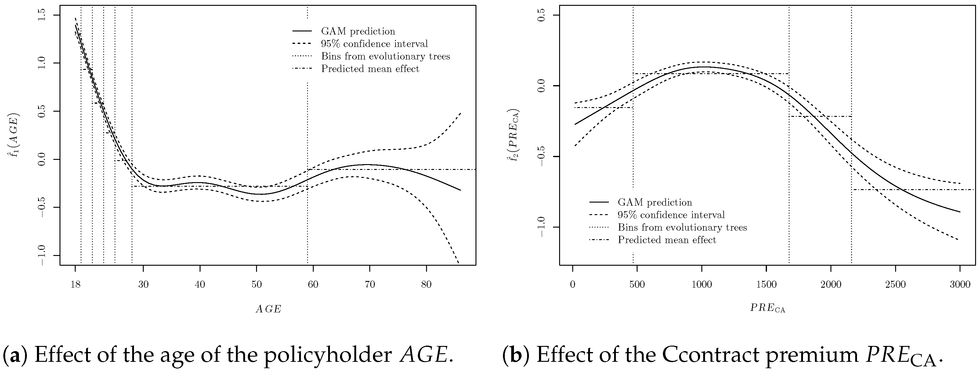
We denote with f ^ 1 and f ^ 2 the empirical fitted smoothing functions of the effects of the age of the policyholder and the CA contract premium, respectively. Figure 6 illustrates both functions revealing nonlinear effects on the cross-selling probability. Dashed lines represent the 95 % confidence intervals, yielding larger intervals in regions where observations are more heterogeneous and scarcer. Indeed, given the shape of the smoothing functions, the variables age A G E and contract premium P R E CA cannot be included as a linear predictor in the Cox model. In Figure 6a, we observe that young customers aged between 18 and 29 years show a higher instantaneous probability of leaving the single-product state, while there is a sharp decrease at lower ages, f ^ 1 is non-monotonic elsewhere yielding only a smaller increase at ages around 60 years. The corresponding effect f ^ 2 from the CA contract premium is monotonically increasing until a value of about CHF 1000 and then decreasing (see Figure 6b).

3.1.3. Binning of Continuous Variables

The Poisson Generalized Linear model does not allow to relate the explanatory variables directly to the time needed to cross-buying (Fuino and Wagner 2020; Kalbfleisch and Prentice 2002). Accelerated failure model (AFT) models allow this relation; however, in the statistical software R that we use, there is no package available which allows smoothing functions to be included (at the time of writing). Traditionally, insurers build categories for continuous variables when the linearity assumption is too restrictive. Dougherty et al. (1995) and Ohlsson and Johansson (2010) propose to group consecutive values to create a category. Henckaerts et al. (2018) propose a machine learning model to build such categories. Accordingly, the continuous variables A G E and P R E CA are segmented in a finite number of classes. We take a data-driven automatic approach by applying evolutionary trees, a machine learning algorithm, on the effects f ^ 1 ( A G E ) and f ^ 2 ( P R E CA ) . In our implementation, we rely on the package evtree in R (Grubinger et al. 2014). The number of leaf nodes , i.e., the number of categories used for each variable, depends on the tuning parameter α through the complexity measure n · log ( M S E ) + 4 · α · ( + 1 ) · log ( n ) , where n is the size of the dataset and M S E the mean squared error. The number of observations n is used as weight in the implementation and we require the calculated bins to contain at least 1000 observations for not being too sparsely populated. Under an increasing penalization parameter α , the number of leaf nodes will decrease. To consider the trade-off between accuracy and complexity of the constructed bins, we replace the continuous variables in the Cox model (3) by the bins and assess the new model using the BIC for each value of α . We retain the bins that bring the smallest BIC value.
The optimal categories for A G E result in the seven classes 18–19, 20–21, 22–23, 23–25, 26–28, 29–59 and 60 + years. The contract premiums are split into four classes: CHF 0–473, 474–1676, 1677–2161 and 2162 + . The boundaries of the bins and the predicted mean effects in each category are illustrated with dashed vertical lines, respectively, dashed-pointed horizontal lines, in the graphs of Figure 6. With the retained binning options our Cox model becomes:
log λ T , x λ 0 ( T ) = β 1 · GEO + β 2 · NCO + β 3 · CHA + β 4 · AGE cat + β 5 · PRE CA , cat ,
where AGE cat and PRE CA , cat correspond to new categorical variables built along the bins reported above.

3.1.4. Accelerated Failure Time Model

To evaluate the relationship between the duration to cross-selling T and the explanatory variables x in an alternative and direct way, we propose to introduce an AFT model. We consider a linear relationship between log T and the covariates as follows:
log T = μ + x β + σ W .
Here μ is a constant and W an error variable based on the inter-purchase time distribution assumption. The observed inter-purchase times T related to the CA policyholders can be empirically fitted to the distributions of a positive random variable. We aim to find the best fit from the exponential, Weibull, Gamma and log-normal distributions (Kalbfleisch and Prentice 2002, chp. 2; Jackson 2016). We chose the best distribution under the BIC measure and compare it to the KM estimates for the cross-selling probabilities. We report along the BIC for the CA cohort and the four considered distributions in Table 3.
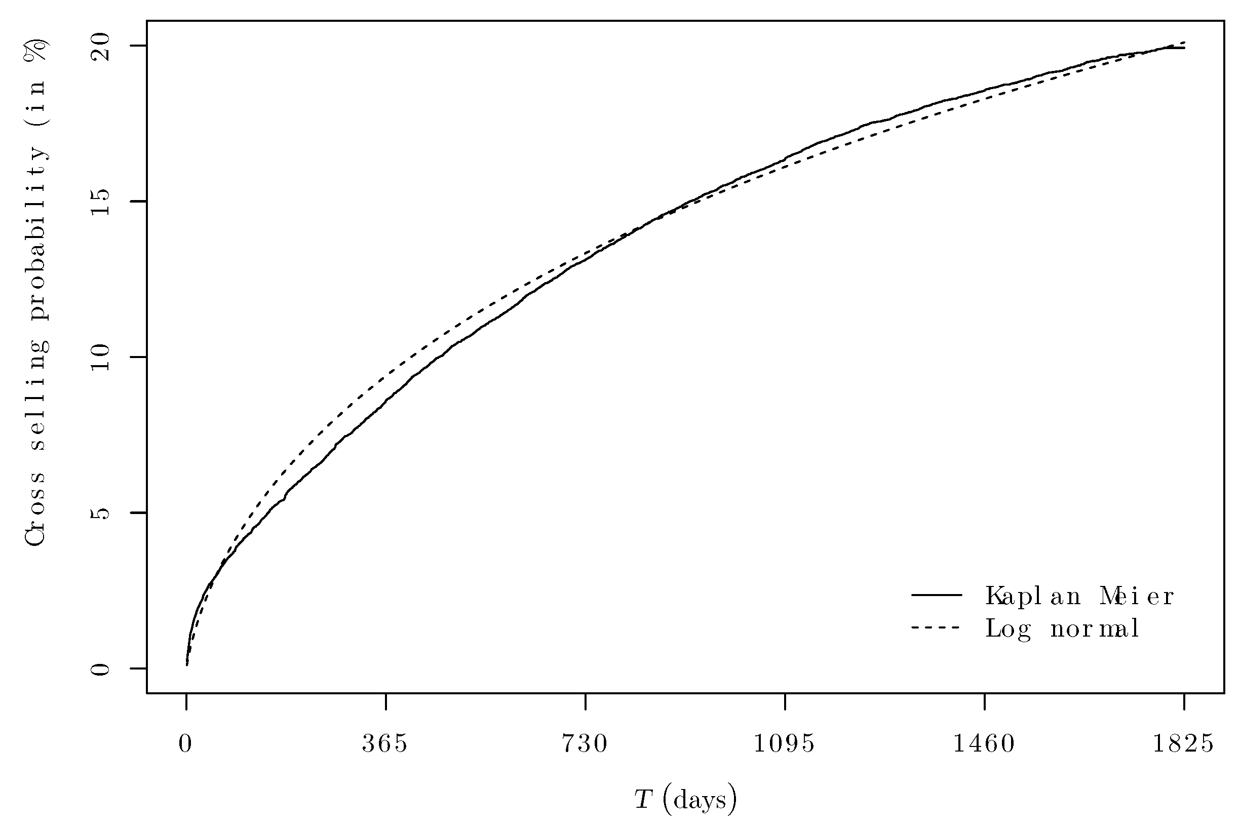
We observe that the log-normal distribution provides the lowest BIC, i.e., the best fit, for describing the cross-selling durations for the CA cohort. Figure 7 illustrates the KM estimate and the fitted log-normal distribution for the CA cohort’s cross-selling times. We observe a good fit by the log-normal distribution for all times above one year in the case of CA (Figure 7). In the following, we remain with the log-normal distribution for describing the cross-selling times. Relying on the optimized right-hand side obtained in Equation (4), we consider the following AFT model:
log T = μ + β 1 · GEO + β 2 · NCO + β 3 · CHA + β 4 · AGE cat + β 5 · PRE CA , cat + σ W .
We use the package survival in R . Note that, for categorical and binary variables, we take the category with the highest number of observations as a baseline.

3.1.5. Numerical Results and Discussion

The application of the Cox and AFT models (4) and (6) on the observations from the CA cohort are summarized in Table 4. For the Cox model, we report the exponential of the estimated β coefficients (column “exp(coeff.)”) as well as the exponential of the standard error (column “exp(s.e.)”). Note that the model provides results for the instantaneous cross-selling probability where smaller, respectively, larger values are inversely related to larger and smaller durations. For easing the interpretation of the duration to cross-selling and for allowing a direct comparison with the AFT model, we also report the inverse exponential value exp ( β ) for the Cox model (column “exp(−coeff.)” highlighted with gray background). Values above, respectively, below one, express longer, respectively, shorter, durations to cross-selling. For the AFT models, we first provide the coefficient and standard error estimates as obtained from the R -routine. In a gray shaded column (“exp(coeff.)”) we provide the exponentiated values of the coefficient that can be directly compared with those obtained in the Cox model. As expected, given the selection procedure for the variables, we observe that all are significant. The results obtained from the Cox model are in line with those obtained from the AFT model and confirm the discussion of the impact of the various factors derived from the descriptive statistics. Through the geographic regions, we observe that customers from the French-(GR) and Italian-speaking regions (GI) present higher cross-selling durations. The duration significantly decreases with an increasing number of contracts NCO . Policyholders underwriting their contracts through a tied agent (baseline of the model) yield the lowest cross-selling times when compared to any other interaction channel. Customers aged between 29 and 59 years (baseline) present the longest times T. Hence, managers should develop marketing actions for customers under 29 years who have access to a tied agent. Especially during times, where information can easily be compared online. We remark a sensitivity to no cross-selling when customers are loosing their student rebates, which is usually given till the age of 25 in Switzerland. Particular efforts in the development are needed in customers with a low premium. The insurer often has low power to develop these customers since they mostly relate to young customers having their first (isolated) contracts with limited needs. The (negative) influence of brokers should also be studied and, e.g., be countered by contacting the customers at the end of their contract duration.

3.2. Model for the HL Cohort

3.2.1. Model Development

Following the sequence from the previous section, we now derive optimal Cox and AFT models to describe the duration to cross-selling for the HL cohort. Using forward and backward stepwise selection on the available variables under the BIC, the Cox model yields:
log λ T , x λ 0 ( T ) = β 1 · U R B + β 2 · NCO + β 3 · CHA + f 1 ( A G E ) + f 2 ( P R E HL ) .
This model can be directly compared with Equation (3), while both models are very close and include the respective contract premium for ( P R E CA or P R E HL ), we observe that the model for the HL cohort includes the binary urbanicity variable U R B in place of the geographic region variable GEO . The other variables are the same in both CA and HL models. If we allow for interactions between the age of the policyholder A G E and the contract premium P R E HL , the model does not improve under the BIC.
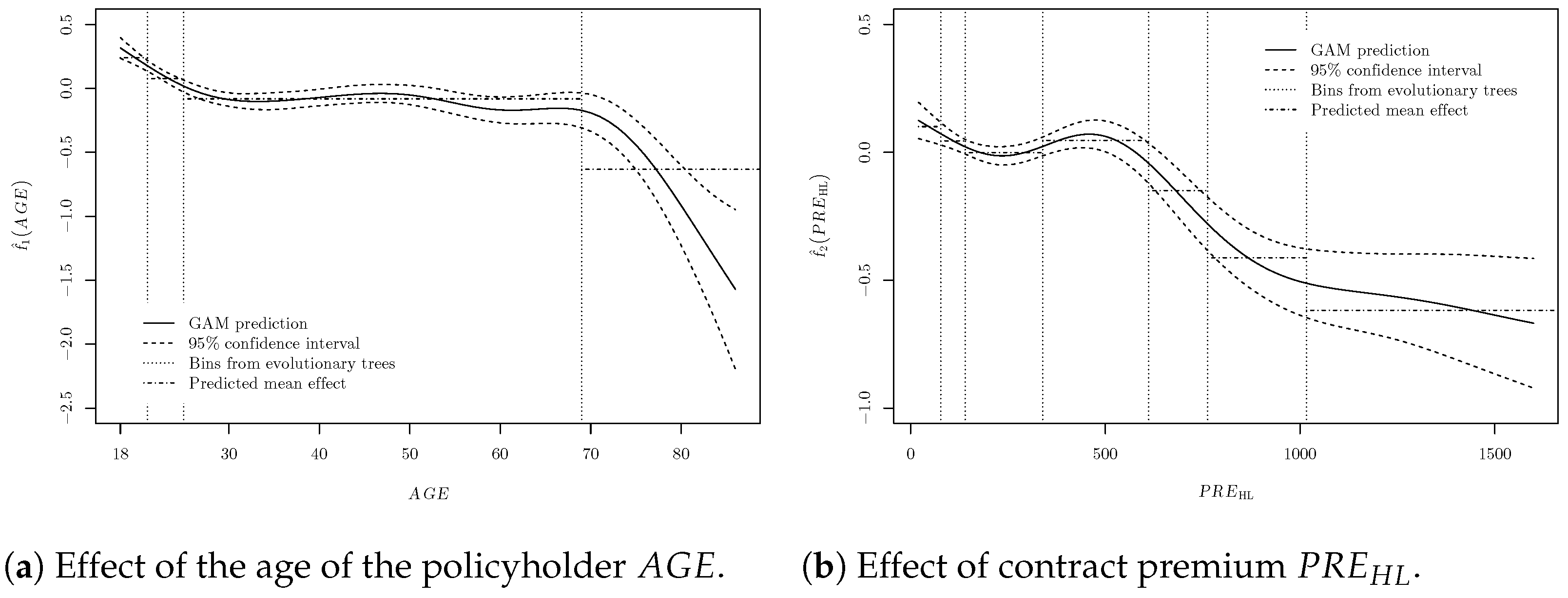
In Figure 8, we illustrate the smoothed effects f ^ 1 ( A G E ) and f ^ 2 ( P R E HL ) of the policyholder age and the contract premium on the cross-selling probability. The shapes of the functions differ from the ones obtained for the CA cohort (cf. Figure 6). In the HL cohort, the influence of younger customers is more limited and only a small decrease is observed in Figure 8a. This may be linked to the specificity of the other product, i.e., car insurance, where cross-buying CA is linked to buying a car. In fact, among young customers, possessing a car is much less common than living in the own household away from the parents. At ages above 70 years, the effect shown by f ^ 1 is negative, resulting in lower instantaneous to cross-selling probabilities. The function f ^ 2 is non-monotonic (see Figure 8b). For lower premiums, we observe only small variations. For a contract premium above about CHF 500, the effect is importantly decreasing. Thus, customers with higher premiums have a higher probability to remain single-product customers. For both the policyholder age and the contract premium the effects seem to be smaller when compared to the findings from the CA cohort.
Further, we derive optimal bins for the continuous variables A G E and P R E HL . Using the evolutionary trees technique, the age of the policyholder variable A G E becomes AGE cat and is binned into four categories, namely, 18–21, 22–25, 26–29 and 70 + years. The HL contract premium PRE HL , cat is categorized along seven bins: CHF 20–80, 81–148, 149–359, 360–578, 579–698, 699–910 and 911 + . We graphically illustrate the retained classes and their effects in Figure 8, while we have retained seven age classes in the CA cohort, we only define four age categories in the case of HL. Conversely, while in the CA cohort we have identified four classes for the contract premium, there are seven in the HL cohort. The age and the premium have a lower, respectively, higher influence, on cross-selling in HL than in CA. In consequence, the final Cox model with only categorical variables becomes:
log λ T , x λ 0 ( T ) = β 1 · U R B + β 2 · NCO + β 3 · CHA + β 4 · AGE cat + β 5 · PRE HL , cat .
Finally, we apply the right-hand side expression of Equation (8) in an AFT model which writes out as follows:
log T = μ + β 1 · U R B + β 2 · NCO + β 3 · CHA + β 4 · AGE cat + β 5 · PRE HL , cat + σ W ,
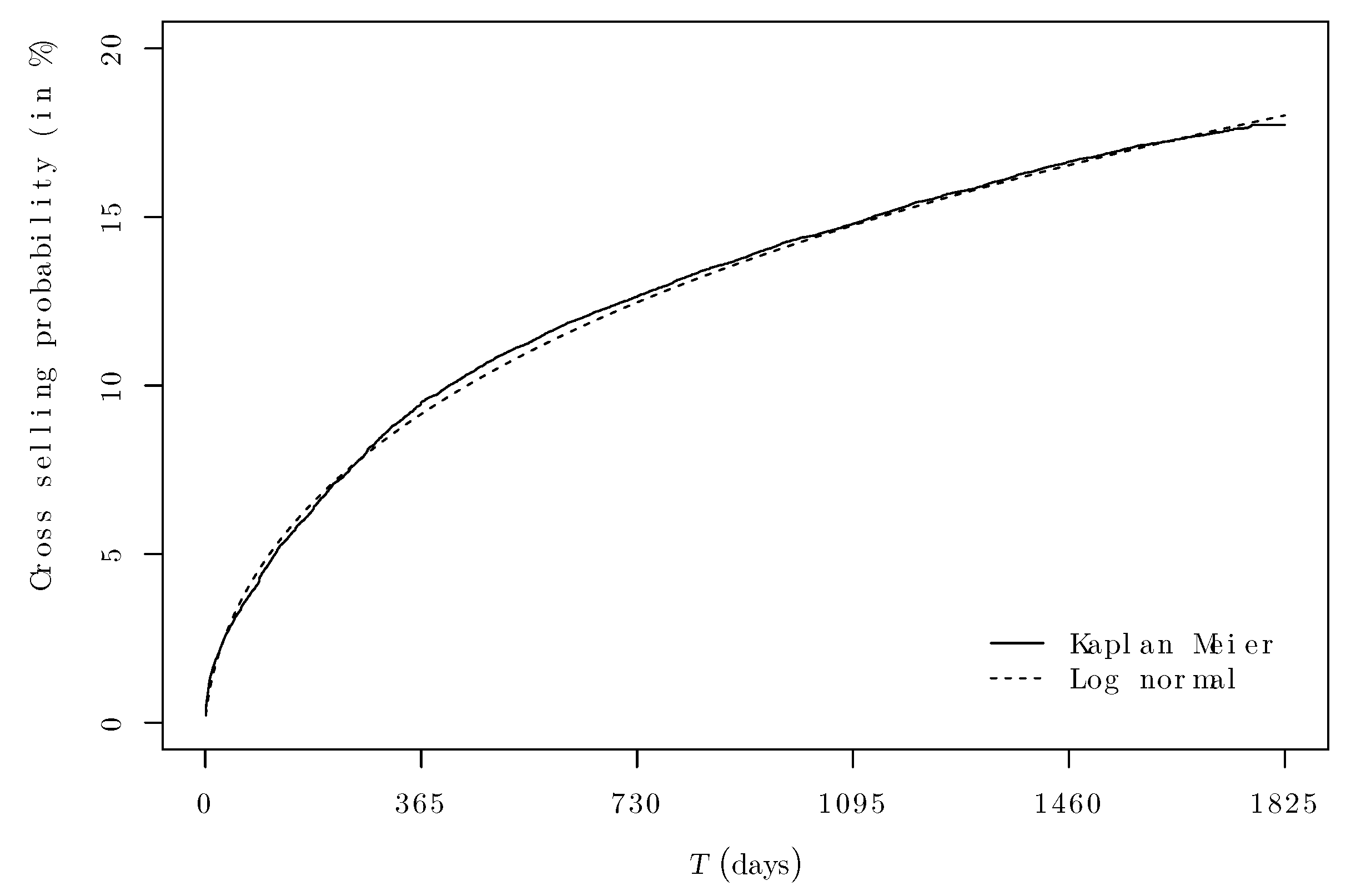
where for W we assume a log-normal distribution according to the BIC measure in Table 5 and Figure 9. We observe a quasi-perfect overlapping throughout all times for the HL cohort.

3.2.2. Numerical Results and Discussion

Following the layout of Table 4, the empirical results from the Cox model (8) and the AFT model (9) are summarized in Table 6. We note that in both models the same coefficients are significant. Customers living in a rural region show smaller transition times and thus are cross-buying faster than customers from urban regions. The duration to cross-selling decreases with the number of contracts and we find that customers initially buying from a tied agent are faster to also hold the CA product when compared to the other access channels. Customer relationships stemming from a broker take significantly longer to develop. Further, we observe that younger customers and those with lower HL contract premiums are faster to buy car insurance. We also show that the relationship of insurers with urban customers are critical. Tied agents could help, but also research on if car cross-selling is an option for urban customers needs to be done. Indeed urban customers may have no need for such cover (e.g., in the absence of car ownership.

4. Conclusions

Only limited research and figures on cross-selling in non-life insurance are available in the literature and, to the best of our knowledge, the factors related to the duration to cross-selling have received little attention in econometric studies. In this paper, we aim to provide insights about the time it takes to develop customer-insurer relationships through cross-selling. Focusing on two non-life insurance products, we study the development of new customer cohorts on the basis of a longitudinal data set. For both car and household-liability insurance customers we identify the factors that significantly relate to the customer development timeline.
We observe different dynamics in both considered cohorts. Relying on Kaplan–Meier estimates, we lay out for the two cohorts the duration it takes to sell the other product to 5%, 10% respectively 15% of the customers. Within the actuarial framework of survival analysis, we further develop a Cox model and an AFT model to describe the probabilities and times to cross-selling. We find that the place of residence, the number of contracts held, the access channel, the age and the contract premiums are significant in describing the duration to cross-selling.
While we are able to quantify the impact of the selected factors for cross-selling, our findings provide a first step for getting a better understanding in insurance customer dynamics. In fact, this is particularly relevant for practitioners as an intermediate step for timing marketing actions. As discussed in, e.g., Staudt and Wagner (2018), relationship management should integrate the whole customer lifecycle. We identify several directions for further research. For example, the inclusion of data about the cancellation of a contract and other products would allow to explain in more detail the customer journey. Calibrating semi-Markov models on historical longitudinal data could provide further probabilistic insights and the relevant factors for retaining existing customers (Janssen and Manca 2006). Moreover, the inclusion of more detailed risk factors and socio-economic variables may improve the modeling. Finally, the prediction power could be enhanced with a longer dataset and the application of more sophisticated methods like random forests.

Author Contributions

Conceptualization, Y.S. and J.W.; methodology, Y.S. and J.W.; investigation, Y.S.; formal analysis, Y.S. and J.W.; data curation, Y.S.; writing—original draft preparation, Y.S.; writing—review and editing, Y.S. and J.W.; supervision, J.W. All authors have read and agreed to the published version of the manuscript.

Funding

The APC was funded by the University of Lausanne.

Data Availability Statement

Not applicable.

Acknowledgments

Both authors are thankful to the insurance company providing the data for the analysis.

Conflicts of Interest

The authors declare no conflict of interest.

Notes

1
GE includes major cities like Zurich and Winterthur, GW includes Berne and Basel, GA includes St. Gallen, Chur and Lucerne, GR includes Geneva, Lausanne and Sion, and GI includes Lugano and Locarno. We denote categorical variables in bold face and, e.g., the vector GEO has the form (GE, GW, GA, GR, GI, OT).
2
We use subscripts CA and HL on P R E to distinguish the premium in both products.
3
As we use rounded quartile values as boundaries for the classes, we find shares not exactly equal to 25%.

References

  1. Aalen, Odd O., Ørnulf Borgan, and Håkon K. Gjessing. 2008. Survival and Event History Analysis. Statistics for Biology and Health. New York: Springer. [Google Scholar] [CrossRef]
  2. Ansell, Jake, Tina Harrison, and Tom Archibald. 2007. Identifying Cross-selling Opportunities, Using Lifestyle Segmentation and Survival Analysis. Marketing Intelligence and Planning 25: 394–410. [Google Scholar] [CrossRef]
  3. Bieck, Christian, Boderas Mareike, Peter Maas, and Tobias Schlager. 2010. Powerful Interaction Points: Saying Goodbye to the Channel. Somers: IBM Institute for Business Value and University of St. Gallen. [Google Scholar]
  4. Denuit, Michel, and Stefan Lang. 2004. Non-life Rate-making with Bayesian GAMs. Insurance: Mathematics and Economics 35: 627–47. [Google Scholar] [CrossRef]
  5. Dougherty, James, Ron Kohavi, and Mehran Sahami. 1995. Supervised and Unsupervised Discretization of Continuous Features. Machine Learning 12: 194–202. [Google Scholar] [CrossRef]
  6. Dutang, Christophe. 2012. Etude des Marchés D’assurance Non-Vie à L’aide D’équilibre de Nash et de Modèle de Risques Avec Dépendance. Doctoral thesis, Université Claude Bernard—Lyon I, Villeurbanne, France. [Google Scholar]
  7. Eling, Martin, and Dieter Kiesenbauer. 2014. What Policy Features determine Life Insurance Lapse? An Analysis of the German Market. The Journal of Risk and Insurance 81: 241–69. [Google Scholar] [CrossRef]
  8. Fornell, Claes, and Birger Wernerfelt. 1987. Defensive Marketing Strategy by Customer Complaint Management: A Theoretical Analysis. Journal of Marketing Research 24: 337–46. [Google Scholar] [CrossRef]
  9. Frees, Edward W. 2015. Analytics of Insurance Markets. Annual Review of Financial Economics 7: 253–77. [Google Scholar] [CrossRef]
  10. Frees, Edward W., Richard A. Derrig, and Glenn Meyers. 2016. Predictive Modeling Applications in Actuarial Science Volume 1: Predictive Modeling Techniques. Cambridge: Cambridge University Press. [Google Scholar] [CrossRef]
  11. Fuino, Michel, and Joël Wagner. 2020. Duration of Long-Term Care: Socio-Economic Drivers, Evolution and Type of Care Interactions. Insurance: Mathematics and Economics 90: 151–168. [Google Scholar] [CrossRef]
  12. Grewal, Rajdeep, Raj Mehta, and Frank R. Kardes. 2004. The Timing of Repeat Purchases of Consumer Durable Goods: The Role of Functional Bases of Consumer Attitudes. Journal of Marketing Research 41: 101–15. [Google Scholar] [CrossRef] [Green Version]
  13. Grubinger, Thomas, Achim Zeileis, and Karl-Peter Pfeiffer. 2014. Evtree: Evolutionary Learning of Globally Optimal Classification and Regression Trees in R. Journal of Statistical Software 61: 1–29. [Google Scholar] [CrossRef]
  14. Guillen, Montserrat, Jens Perch Nielsen, and Ana M. Pérez-Marín. 2008. The Need to Monitor Customer Loyalty and Business Risk in the European Insurance Industry. The Geneva Papers on Risk and Insurance—Issues and Practice 33: 207–18. [Google Scholar] [CrossRef]
  15. Gupta, Sunil, Dominique Hanssens, Bruce Hardie, William Kahn, V. Kumar, Nathaniel Lin, Nalini Ravishanker, S. Sriram, Dominique Hanssens, and W. Kahn. 2006. Modeling Customer Lifetime Value. Journal of Service Research 9: 139–55. [Google Scholar] [CrossRef]
  16. Henckaerts, Roel, Katrien Antonio, Maxime Clijsters, and Roel Verbelen. 2018. A Data Driven Binning Strategy for the Construction of Insurance Tariff Classes. Scandinavian Actuarial Journal 2018: 681–705. [Google Scholar] [CrossRef]
  17. Jackson, Christopher. 2016. flexsurv: A Platform for Parametric Survival Modeling in R. Journal of Statistical Software 70: 1–33. [Google Scholar] [CrossRef] [PubMed]
  18. Jain, Dipak C., and Naufel J. Vilcassim. 1991. Investigating Household Purchase Timing Decisions: A Conditional Hazard Function Approach. Marketing Science 10: 1–23. [Google Scholar] [CrossRef]
  19. James, Gareth, Daniela Witten, Trevor Hastie, and Robert Tibshirani. 2013. An Introduction to Statistical Learning with Applications in R. New York: Springer. [Google Scholar] [CrossRef]
  20. Janssen, Jacques, and Raimondo Manca. 2006. Applied Semi-Markov Processes. New York: Springer. [Google Scholar]
  21. Kalbfleisch, John D., and Ross L. Prentice. 2002. The Statistical Analysis of Failure Time Data. Wiley Series in Probability and Statistics; Hoboken: John Wiley & Sons, Inc. [Google Scholar] [CrossRef]
  22. Kamakura, Wagner A. 2007. Cross-Selling: Offering the Right Product to the Right Customer at the Right Time. Journal of Relationship Marketing 6: 41–58. [Google Scholar] [CrossRef]
  23. Kamakura, Wagner A., Michel Wedel, Fernando de Rosa, and Jose Afonso Mazzon. 2003. Cross-Selling through Database Marketing: A Mixed Data Factor Analyzer for Data Augmentation and Prediction. International Journal of Research in Marketing 20: 45–65. [Google Scholar] [CrossRef] [Green Version]
  24. Klein, Nadja, Michel Denuit, Stefan Lang, and Thomas Kneib. 2014. Nonlife Ratemaking and Risk Management with Bayesian Generalized Additive Models for Location, Scale, and Shape. Insurance: Mathematics and Economics 55: 225–49. [Google Scholar] [CrossRef]
  25. Knott, Aaron, Andrew Hayes, and Scott A. Neslin. 2002. Next-Product-to-Buy Models for Cross-Selling Applications. Journal of Interactive Marketing 16: 59–75. [Google Scholar] [CrossRef]
  26. Kumar, Vikas, Morris George, and Joseph Pancras. 2008. Cross-Buying in Retailing: Drivers and Consequences. Journal of Retailing 84: 15–27. [Google Scholar] [CrossRef]
  27. Laas, Daniela, Hato Schmeiser, and Joël Wagner. 2016. Empirical Findings on Motor Insurance Pricing in Germany, Austria and Switzerland. The Geneva Papers on Risk and Insurance—Issues and Practice 41: 398–431. [Google Scholar] [CrossRef]
  28. Lüdi, Georges, and Iwar Werlen. 2005. Sprachenlandschaft in der Schweiz. Neuchâtel: Swiss Federal Statistical Office. [Google Scholar]
  29. Maas, Peter, Albert Graf, and Christian Bieck. 2008. Trust, Transparency and Technology. Somers: IBM Institute for Business Value and University of St. Gallen. [Google Scholar]
  30. Mau, Stefan, Irena Pletikosa Cvijikj, and Joël Wagner. 2015. From Research to Purchase: An Empirical Analysis of Research-shopping Behaviour in the Insurance Sector. Zeitschrift für die Gesamte Versicherungswissenschaft 104: 573–93. [Google Scholar] [CrossRef]
  31. Mau, Stefan, Irena Pletikosa Cvijikj, and Joël Wagner. 2017. Insurance Consumption and Customer Portfolio Characteristics in Multichannel Distribution: New Empirical Evidence. Working Paper. Lausanne: University of Lausanne. [Google Scholar]
  32. Mau, Stefan, Irena Pletikosa Cvijikj, and Joël Wagner. 2018. Forecasting the Next Likely Purchase Events of Insurance Customers. International Journal of Bank Marketing 36: 1125–44. [Google Scholar] [CrossRef]
  33. Moore, Dirk F. 2016. Applied Survival Analysis Using R Use R! Cham: Springer International Publishing. [Google Scholar] [CrossRef]
  34. Ngobo, Paul Valentin. 2004. Drivers of Customers’ Cross-Buying Intentions. European Journal of Marketing 38: 1129–57. [Google Scholar] [CrossRef]
  35. Ohlsson, Esbjörn, and Björn Johansson. 2010. Non-Life Insurance Pricing with Generalized Linear Models. EAA SERIES. Berlin/Heidelberg: Springer. [Google Scholar] [CrossRef]
  36. Prinzie, Anita, and Dirk Van den Poel. 2006. Investigating Purchasing-Sequence Patterns for Financial Services using Markov, MTD and MTDg Models. European Journal of Operational Research 170: 710–34. [Google Scholar] [CrossRef]
  37. Prinzie, Anita, and Dirk Van den Poel. 2007. Predicting Home-appliance Acquisition Sequences: Markov/Markov for Discrimination and Survival Analysis for Modeling Sequential Information in NPTB models. Decision Support Systems 44: 28–45. [Google Scholar] [CrossRef]
  38. Schwarz, Gideon. 1978. Estimating the Dimension of a Model. The Annals of Statistics 6: 461–64. [Google Scholar] [CrossRef]
  39. Staudt, Yves, and Joël Wagner. 2018. What Policyholder and Contract Features Determine the Evolution of Non-life Insurance Customer Relationships? A Case Study Analysis. International Journal of Bank Marketing 36: 1098–124. [Google Scholar] [CrossRef]
  40. Staudt, Yves, and Joël Wagner. 2019. Comparison of Machine Learning and Traditional Severity-Frequency Regression Models for Car Insurance Pricing. Working Paper. Lausanne: University of Lausanne. [Google Scholar]
  41. Verhoef, Peter C., and Bas Donkers. 2005. The Effect of Acquisition Channels on Customer Loyalty and Cross-Buying. Journal of Interactive Marketing 19: 31–43. [Google Scholar] [CrossRef]
  42. Verhoef, Peter C., Philip Hans Franses, and Janny C. Hoekstra. 2001. The Impact of Satisfaction and Payment Equity on Cross-Buying: A Dynamic Model for a Multi-Service Provider. Journal of Retailing 77: 359–78. [Google Scholar] [CrossRef]
  43. Whitehead, John. 1980. Fitting Cox’s Regression Model to Survival Data using GLIM. Applied Statistics 29: 268. [Google Scholar] [CrossRef]
  44. Wood, Simon N. 2017. Generalized Additive Models: An Introduction with R, 2nd ed. Boca Raton: CRC Press. [Google Scholar]
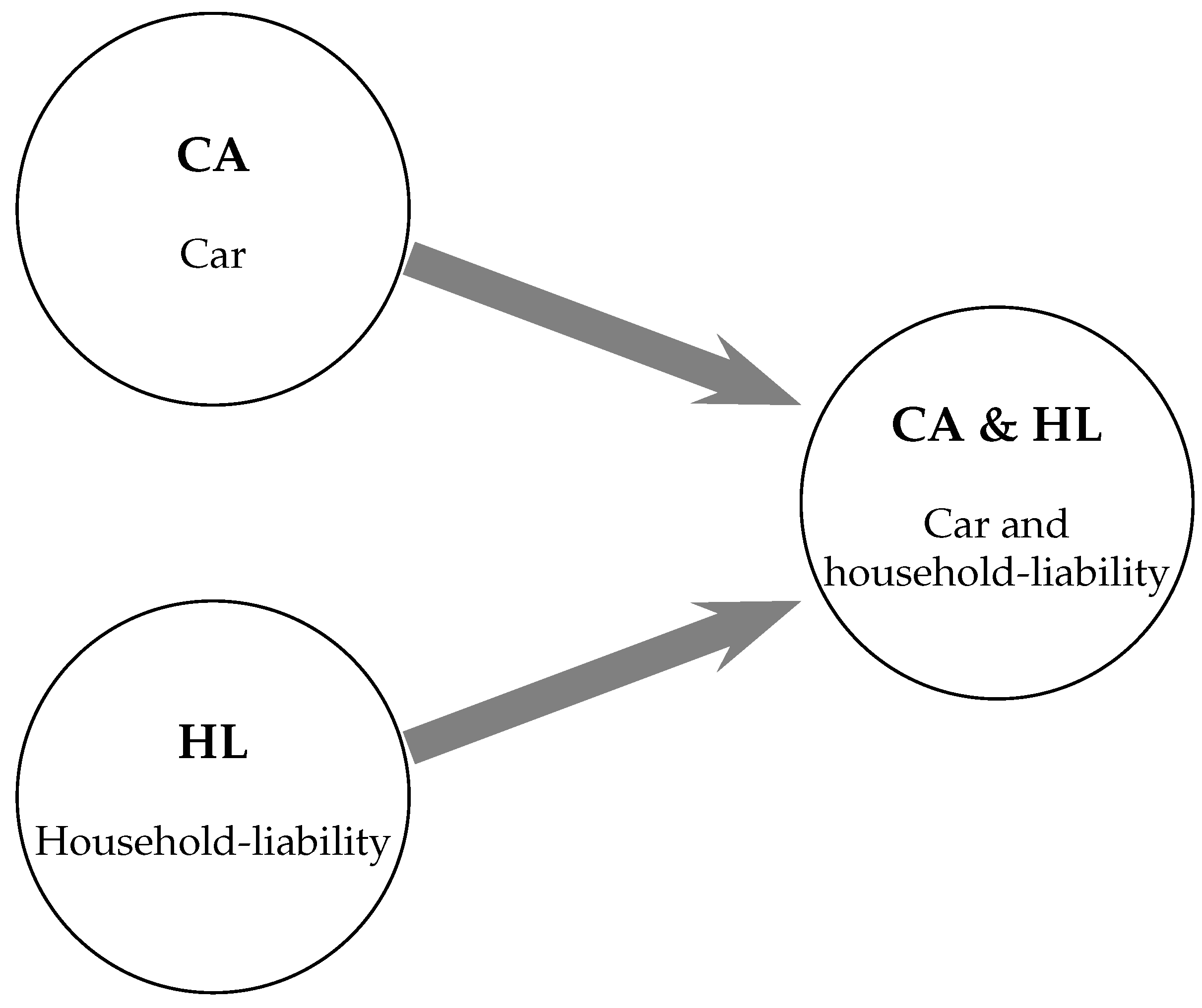
Figure 1. Illustration of the states and transitions considered.
Risks 10 00187 g001
Figure 2. Illustration of the portfolio development.
Risks 10 00187 g002
Figure 3. Kaplan–Meier estimates for the cross-selling probability for the CA and HL cohorts. The gray shaded area indicates the 95% confidence interval of the estimate.
Risks 10 00187 g003
Figure 4. Illustration of the relative frequencies along covariates in the CA cohort.
Risks 10 00187 g004
Figure 5. Illustration of the relative frequencies along covariates in the HL cohort.
Risks 10 00187 g005
Figure 6. Illustration of the prediction effect from the Cox model ( f ^ 1 and f ^ 2 ) in Equation (3) and of the bins obtained from evolutionary trees for the age of the policyholder A G E and the contract premium P R E CA in the CA cohort.
Risks 10 00187 g006
Figure 7. Kaplan–Meier estimates for the cross-selling probability and log-normal distribution fit for the CA cohort.
Risks 10 00187 g007
Figure 8. Illustration of the prediction effect from the Cox model ( f ^ 1 and f ^ 2 ) in Equation (7) and of the bins obtained from evolutionary trees for the age of the policyholder A G E and the contract premium P R E HL in the HL cohort.
Risks 10 00187 g008
Figure 9. Kaplan–Meier estimates for the cross-selling probability and log-normal distribution fit for the HL cohort.
Risks 10 00187 g009
Table 1. Summary of the variables available in the data.
VariableDescription
Customer attributes
    A G E Age of the policyholder
    U R B Urbanicity of the residence: urban (UU) or rural (UR)
    GEO Geographic region of the residence:
– East Swiss Plateau (GE)
– West Swiss Plateau (GW)
– Alps and Prealps (GA)
– Romandy (GR)
– Italian-speaking area of Switzerland (GI)
– Outside of Switzerland (OT)
Products attributes
    P R E CA or HL contract premium paid (in CHF)
    NDA Number of damages declared (0, 1, 2, 3+)
    NCO Number of contracts underwritten (1, 2, 3, 4+)
    L I F Life insurance underwritten (yes or no)
Buying channel attribute
    CHA Access channel used by the policyholder:
– Tied agent (TA)
– Independent intermediary (IY)
– Broker (BR)
– Internet/insurer’s website (IT)
– Other (OT)
Table 2. Shares (in %) and T 5 % , T 10 % , T 15 % inter-purchase time quantiles (in days) along covariates.
CA CohortHL Cohort
Share T 5 % T 10 % T 15 % Share T 5 % T 10 % T 15 %
Age (AGE, in years)
 18–25 22.3 40189349 38.9 122412919
 26–40 34.4 2217621683 28.8 1114231348
 41–65 38.2 250781n.a 27.2 1123651226
 66+ 5.1 257031231 5.1 179853n.a.
Urbanicity (URB)
 Urban (UU) 31.7 1906161218 42.3 205849n.a.
 Rural (UR) 68.3 137416819 57.7 89289719
Geographic region ( GEO )
 East Swiss Plateau (GE) 26.0 1595091001 26.6 1224511168
 West Swiss Plateau (GW) 22.9 118380710 26.5 1264161156
 Alps and Prealps (GA) 24.6 108365720 26.0 96325822
 Romandy (GR) 19.2 2146091370 16.7 1535891641
 Italian-speaking area (GI) 6.8 3961223n.a. 3.6 1225501382
 Outside Switzerland (OT) 0.6 179481759 0.5 3496216
CA contract premium (PRE CA , in CHF)
 0–747 25.0 2126541380
 748–1068 25.0 137441869
 1069–1405 25.0 128404762
1406 + 25.0 147418853
HL contract premium (PRE HL , in CHF)
 0–109 25.8 117397901
 110–252 24.4 201868n.a.
 253–391 24.9 1124091233
392 + 25.0 92275699
Number of damages ( NDA )
 0 88.0 158478955 96.7 1184131137
 1 9.4 95365758 3.0 112349792
 2 2.1 113365763 0.3 456820n.a.
3 + 0.5 85314478 0.0 88412641264
Number of contracts ( NCO )
 1 89.3 4799311774 87.9 4751207n.a.
 2 9.5 3715 10.8 3717
 3 1.0 61219 1.1 41117
4 + 0.2 2731 0.2 6837
Life insurance underwritten (LIF)
 No 98.8 152470933 98.6 1204271161
 Yes 1.2 40189522 1.4 92165253
Access channel ( CHA )
 Tied agent (TA) 65.7 114365708 79.5 109372977
 Independent intermediary (IY) 17.0 1626171214 11.5 1484621720
 Broker (BR) 14.1 5241676n.a. 7.8 2641343n.a.
 Internet/insurer’s website (IT) 1.4 144438704 0.0 n.a.n.a.n.a.
 Other (OT) 1.7 475n.a.n.a. 1.1 112932n.a.
n.a. stands for not applicable.
Table 3. Goodness-of-fit statistics (BIC) of the cross-selling times T for the CA cohort.
DistributionExponentialWeibullGammaLog-Normal
CA cohort108,385106,309106,332106,306
Table 4. Empirical results of the Cox and AFT models (4) and (6) for the CA cohort.
Cox Model (4)AFT Model (6)
exp(coeff.)exp(s.e.) exp(−coeff.)coeff.s.e. exp(coeff.)
Geographic region ( GEO )
 East Swiss Plateau (GE)Baseline Baseline
 West Swiss Plateau (GW) 1.135 0.038 * * * 0.881 0.170 0.057 * * 0.844
 Alps and Prealps (GA) 1.150 0.037 * * * 0.870 0.153 0.056 * * 0.859
 Romandy (GR) 0.924 0.044 .1.082 0.065 0.063 1.067
 Italian-speaking area (GI) 0.743 0.074 * * * 1.345 0.390 0.100 * * * 1.477
 Outside Switzerland (OT) 1.176 0.171 0.851 0.474 0.259 . 0.622
Number of contracts ( NCO )
 1Baseline
 2 9.018 0.032 * * * 0.111 4.017 0.058 * * * 0.018
 3 13.475 0.078 * * * 0.074 4.415 0.150 * * * 0.012
4 + 15.947 0.152 * * * 0.063 4.764 0.297 * * * 0.009
Access channel ( CHA )
 Tied agent (TA)Baseline Baseline
 Independent intermediary (IY) 0.926 0.039 * 1.080 0.128 0.056 * 1.136
 Broker (BR) 0.567 0.054 * * * 1.765 0.754 0.070 * * * 2.125
 Internet/insurer’s website (IT) 0.972 0.105 1.029 0.062 0.158 0.940
 Other (OT) 0.329 0.152 * * * 3.040 1.568 0.199 * * * 4.799
Age ( AGE cat , in years)
 18–19 4.777 0.040 * * * 0.209 2.127 0.071 * * * 0.119
 20–21 3.567 0.046 * * * 0.280 1.706 0.077 * * * 0.182
 22–23 2.578 0.053 * * * 0.388 1.316 0.081 * * * 0.268
 24–25 1.603 0.061 * * * 0.624 0.681 0.090 * * * 0.506
 26–28 1.147 0.057 * 0.872 0.184 0.079 * 0.832
 29–59Baseline Baseline
60 + 1.181 0.051 * * * 0.847 0.144 0.071 * 0.866
CA contract premium ( PRE CA , cat , in CHF)
 18–473 0.754 0.049 * * * 1.327 0.420 0.070 * * * 1.522
 474–1676Baseline Baseline
 1677–2161 0.708 0.049 * * * 1.413 0.405 0.074 * * * 1.499
2162 + 0.430 0.068 * * * 2.327 1.143 0.101 * * * 3.136
μ 10.185 0.059 * * * 26,496
σ 0.835 0.011 * * * 2.305
Significance levels for p-values: *** p ≤ 0.001, ** p ≤ 0.01, * p ≤ 0.05, . p ≤ 0.1. s.e. stands for standard error.
Table 5. Goodness-of-fit statistics (BIC) of the cross-selling times T for the HL cohort.
DistributionExponentialWeibullGammaLog-Normal
CA cohort108,385106,309106,332106,306
HL cohort111,327107,822107,867107,652
Table 6. Empirical results of the Cox and AFT models (8) and (9) for the HL cohort.
Cox Model (8)AFT Model (9)
exp(coeff.)exp(s.e.) exp(−coeff.)coeff.s.e. exp(coeff.)
Urbanicity ( U R B )
    Urban (UU)Baseline Baseline
    Rural (UR) 1.468 0.029 * * * 0.681 0.627 0.049 * * * 0.534
Number of contracts ( NCO )
    1Baseline
    2 9.001 0.030 * * * 0.111 4.550 0.064 * * * 0.011
    3 17.605 0.068 * * * 0.057 5.435 0.160 * * * 0.004
    4 + 14.453 0.159 * * * 0.069 5.068 0.361 * * * 0.006
Access channel ( CHA )
    Tied agent (TA)Baseline Baseline
    Independent intermediary (IY) 0.952 0.045 1.050 0.155 0.075 * 1.167
    Broker (BR) 0.682 0.064 * * * 1.466 0.670 0.100 * * * 1.955
    Internet/insurer’s website (IT) 1.003 1.001 0.997 0.476 1.682 0.621
    Other (OT) 0.406 0.157 * * * 2.466 1.517 0.253 * * * 4.557
Age ( AGE cat , in years)
    18–21 1.291 0.042 * * * 0.775 0.453 0.074 * * * 0.636
    22–25 1.036 0.042 0.966 0.064 0.071 0.938
    26–69Baseline Baseline
    70 + 0.630 0.100 * * * 1.588 0.641 0.153 * * * 1.899
HL contract premium ( PRE H L , cat , in CHF)
    20–80 1.231 0.044 * * * 0.813 0.277 0.077 * * * 0.758
    81–148 1.016 0.046 0.984 0.005 0.076 1.005
    149–359Baseline Baseline
    360–578 1.046 0.039 0.956 0.173 0.067 * * 0.841
    579–698 0.967 0.075 1.035 0.215 0.132 0.807
    699–910 0.642 0.078 * * * 1.557 0.491 0.137 * * * 1.633
    911 + 0.559 0.068 * * * 1.789 0.678 0.119 * * * 1.970
μ 11.206 0.071 * * * 73,553
σ 1.013 0.011 * * * 2.755
Significance levels for p-values: *** p ≤ 0.001, ** p ≤ 0.01, * p ≤ 0.05. s.e. stands for standard error.
Publisher’s Note: MDPI stays neutral with regard to jurisdictional claims in published maps and institutional affiliations.