Probability Density of Lognormal Fractional SABR Model ^†

Abstract

Instantaneous volatility of logarithmic return in the lognormal fractional SABR model is driven by the exponentiation of a correlated fractional Brownian motion. Due to the mixed nature of driving Brownian and fractional Brownian motions, probability density for such a model is less studied in the literature. We show in this paper a bridge representation for the joint density of the lognormal fractional SABR model in a Fourier space. Evaluating the bridge representation along a properly chosen deterministic path yields a small time asymptotic expansion to the leading order for the probability density of the fractional SABR model. A direct generalization of the representation of joint density often leads to a heuristic derivation of the large deviations principle for joint density in a small time. Approximation of implied volatility is readily obtained by applying the Laplace asymptotic formula to the call or put prices and comparing coefficients.

1. Introduction

The celebrated Black and Black-Scholes-Merton models have been the benchmark for European options on currency exchange, interest rates, and equities since the inauguration of the trading on financial derivatives. However, empirical evidence has shown that the main drawback of these models is the assumption of constant volatility; the key parameter required in the calculation of option premia under such models. The volatility parameters induced from market data are in fact nonconstant across markets; dubbed as volatility smile.

The Stochastic $\alpha \beta \rho$ (SABR hereafter) model, suggested by Hagan, Lesniewski, and Woodward in Hagan et al. (2015), is one of the models, such as local volatility models, stochastic volatility models, and exponential Lévy type of models, etc, that attempts to capture the volatility smile effect. Furthermore, as opposed to local volatility models, in the SABR model the volatility smile moves in the same direction as the underlying with time, see Hagan et al. (2002).

The SABR model is depicted by the following system of stochastic differential equations (SDEs):

$$\begin{array}{ccc}& & d{F}_t={\alpha }_t{F}_t^{\beta }d{W}_t,F_0=F,\hfill \end{array}$$

(1)

$$\begin{array}{ccc}& & d{\alpha }_t=\nu {\alpha }_{t}d{Z}_t,{\alpha }_0=\alpha ,\hfill \end{array}$$

(2)

with $\beta \in [0,1]$, where $F_t$ denotes the forward price and ${\alpha }_t$ the instantaneous volatility. $W_t$ and $Z_t$ are correlated Brownian motions with a constant correlation coefficient $\rho$. The SABR model is at times referred to as lognormal SABR when $\beta =1$. The SABR formula is an asymptotic expansion for the implied volatilities of call options with various strikes with small expiry times. For the reader’s convenience, we reproduce the SABR formula in the following. Let ${\sigma }_{BS}(K,\tau )$ be the implied volatility of a vanilla option struck at K and time to expiry $\tau$. The SABR formula states

$${\sigma }_{BS}(K,\tau )=\nu \frac{log(F/K)}{D\left(\zeta \right)}\left\{1+O\left(\tau \right)\right\}$$

(3)

as the time to expiry $\tau$ approaches 0. The function D and the parameter $\zeta$ involved in (3) are defined respectively as

$$D\left(\zeta \right)=log\left(\frac{\sqrt{1-2\rho \zeta +{\zeta }^2}+\zeta -\rho }{1-\rho }\right)$$

and

$$\zeta =\left\{\begin{array}{cc}\frac{\nu }{\alpha }\frac{F^{1-\beta }-K^{1-\beta }}{1-\beta }\hfill & \mathrm{if} \beta \ne 1;\hfill \\ & \\ \frac{\nu }{\alpha }log\left(\frac{F}{K}\right)\hfill & \mathrm{if} \beta =1.\hfill \end{array}\right.$$

Generally, the SABR formula is given one order higher, up to order $\tau$. Here we present only the zeroth order for our own purpose.

The geometry of the SABR model is isometrically diffeomorphic to the two-dimensional hyperbolic space, also known as the Poincaré plane. This isometry leads to a derivation of the SABR Formula (3) based on an expression of the heat kernel, known as the McKean kernel, on Poincaré plane. In particular, the lowest order term in (3) has a geometric interpretation. The function D is the geodesic distance from the spot value $(F_0,{\alpha }_0)$ to the vertical line $F=K$ in the upper half plane $\{(F,\alpha )\in {\mathbb{R}}^2:\alpha \ge 0\}$. Hence, the lowest order term in (3) is indeed the ratio between the absolute value of logmoneyness, i.e., $log(K/F_0)$, and the geodesic distance from $(F_0,{\alpha }_0)$ to the vertical line $F=K$ in the upper half-plane. We refer readers interested in this topic to Hagan et al. (2015) for more detailed discussions. As expression for heat kernel on hyperbolic space is concerned, Ikeda and Matsumoto in Ikeda and Matsumoto (1999) provided a probabilistic approach and obtained, among other interesting results, a representation for the transition density of hyperbolic Brownian motion, i.e., the heat kernel over the Poincaré plane. See Theorem 2.1 in Ikeda and Matsumoto (1999) for details.

The aforementioned nice isometry between the SABR model and Poincaré plane breaks down if the volatility process, i.e., the ${\alpha }_t$ process in (1), is driven by a fractional Brownian motion such as the second equation in (6) considered in the paper. Moreover, due to the lack of Markovianity of fractional Brownian motions, thus the nonexistence of the forward and backward Kolmogorov equations, the classical asymptotic expansion approaches, such as the heat kernel or WKB expansion, are no longer applicable. In this regard, the probabilistic approach in Ikeda and Matsumoto (1999) is more applicable and tractable when dealing with processes driven by fractional Brownian motions.

The volatility process is generally conceived as behaving “fractionally” in that the driving noise is a fractional process, e.g., a fractional Brownian motion with a Hurst exponent other than a half. For a far from an exhaustive list, models that attempt to incorporate the fractional feature of volatility include: the ARFIMA model in Granger and Joyeux (1980) and the FIGARCH model Baillie et al. (1996) for discrete-time models; the long memory stochastic volatility model in Comte and Renault (1998) and the affine fractional stochastic volatility model in Comte et al. (2012) for continuous time models. Somewhat on the contrary, in a recent study in Gatheral et al. (2018), the Hurst exponent H is estimated as being less than a half; thereby indicating antipersistency as opposed to the persistency of the volatility process. For a more detailed and in-depth consideration of this issue, we refer interested readers to the discussions in Cont and Das (2022) and Rogers (2019). It is also worth mentioning that generalizations of the Heston model to the fractional version have been considered in El Euch and Rosenbaum (2019) and Guennoun et al. (2018). Heston-related models are usually dealt with via the characteristic or moment-generating functions. However, in this paper, we take the approach following closely the methodology in Ikeda and Matsumoto (1999). As arbitrage in the modeling is concerned, we remark that, in contrast with the models discussed in for instance Jarrow et al. (2009) and Mishura (2008) within which the underlying prices were assumed driven by fractional Brownian motions, the model considered in the paper is free of arbitrage opportunity since it is the volatility process that is driven by a fractional Brownian motion while the underlying itself is still driven by a (correlated) Brownian motion.

In order to embed the empirically observed fractional feature of the volatility process into the classical SABR model, we suggest in this paper a fractional version of the SABR model as in (6). Modulo a mean-reversion component, this model aligns with the model statistically tested in Gatheral et al. (2018). The main observation in Gatheral et al. (2018) is that in using the square root of the realized variance as a proxy for the instantaneous volatility, the logarithm of the volatility process behaves like a fractional Brownian motion in almost any time scale of frequency. The Hurst exponent H inferred from the time series data is less than a half; indeed, $H\approx 0.1$, see also Cont and Das (2022) and Rogers (2019). This observation of a small Hurst exponent in the volatility process analyzes the model as more technical and challenging from a stochastic analysis point of view. To our knowledge, most of the small time asymptotic expansions for processes driven by fractional Brownian motions have restrictions on the Hurst exponent H of the driving fractional Brownian motion, mostly $H\ge \frac{1}{4}$. One of the advantages of the approach undertaken in the current paper is that it works without restriction on the Hurst exponent H. The key ingredient is a representation in a Fourier space, which we call the bridge representation in Section 2, for the joint density of log spot and volatility, see (9).

A small time asymptotic expansion of the joint density is readily obtained from the bridge representation. The idea is to approximate the conditional expectation in the bridge representation by a judiciously chosen deterministic path since, conditioned on the initial and terminal points, at each point in time a Gaussian process will not wander too far away from its expectation. As long as an asymptotic expansion for the density of the underlying asset is available, obtaining an expansion for implied volatility is almost straightforward by basically comparing the coefficients with a similar expansion obtained by using the lognormal density on the Black or the Black-Scholes-Merton side.

The methodology of deriving the bridge representation (9) can be generalized directly to obtain a bridge representation for the joint density multiple times; hence inducing a representation for finite-dimensional distributions of the fractional SABR model, see Theorem 4. Based on this bridge representation for finite-dimensional distributions, Section 5 is devoted to a heuristic yet appealing derivation of the large deviations principle for the joint density of the fractional SABR model in small time. This large deviations principle in a sense can be regarded as defining a “geodesic distance” over the fractional SABR plane since, as we shall show in Section 5, it recovers the energy functional on the Poincaré plane when $H=\frac{1}{2}$. We leave the rigorous proof of the large deviations principle in future work. An immediate consequence of this large deviation principle is the fractional SABR formula (to the lowest order) (26) which recovers the classical SABR formula when $H=\frac{1}{2}$. The fractional SABR Formula (26) pertains to the guiding principle that the lowest order term in the implied volatility expansion is given by the ratio between the absolute value of the logmoneyness and the geodesic distance to the vertical line $F=K$.

The rest of the paper is organized as follows. The fractional SABR model is specified and the bridge representation for joint density is shown in Section 2. Section 3 and Section 4 provide small time asymptotic expansions of the joint density and of the implied volatilities respectively. Section 5 presents the bridge representation for finite-dimensional distributions and the large deviations principle. Finally, the paper concludes in Section 6 with discussions.

2. Model Specification

Throughout the text, $B=\{B_t,t\ge 0\}$ and $W=\{W_t,t\ge 0\}$ denote two independent standard Brownian motions defined on the filtered probability space $(\Omega ,{\mathcal{F}}_t,\mathbb{P})$ satisfying the usual conditions. Let $B^H=\{B_t^H,t\ge 0\}$ be a fractional Brownian motion with Hurst exponent $H\in (0,1)$ generated by B (see Decreusefond and Üstünel 1999), i.e.,

$$B_t^H={\int }_0^t{K}_H(t,s)d{B}_s,$$

where $K_H$ is the Molchan-Golosov kernel

$$K_H(t,s)=c_H{(t-s)}^{H-\frac{1}{2}}F\left(H-\frac{1}{2},\frac{1}{2}-H,H+\frac{1}{2};1-\frac{t}{s}\right){\mathbf{1}}_{[0,t]}\left(s\right),$$

(4)

with $c_H={\left[\frac{2H\Gamma \left(\frac{3}{2}-H\right)}{\Gamma (2-2H)\Gamma \left(H+\frac{1}{2}\right)}\right]}^{1/2}$ and F is the Gauss hypergeometric function. Also, the autocovariance function of a fractional Brownian motion is denoted by $R(t,s)$ and defined as

$$R(t,s)=\mathbb{E}\left(B_t^H{B}_s^H\right)=\frac{1}{2}\left(t^{2H}+s^{2H}-{|t-s|}^{2H}\right).$$

(5)

Lastly, we assume that all random variables and stochastic processes are defined on $(\Omega ,{\mathcal{F}}_t,\mathbb{P})$.

2.1. The Model

We study the following lognormal fractional SABR (fSABR hereafter) model in risk-neutral probability (for simplicity, interest and dividend rates are both assumed zero):

$$\left\{\begin{array}{c}{S}_t=s_0+{\int }_0^t{\alpha }_r{S}_r(\rho d{B}_r+\overline{\rho }d{W}_r),\hfill \\ \\ {\alpha }_t={\alpha }_0{e}^{\nu B_t^H},\hfill \end{array}\right.$$

(6)

where $s_0$ and ${\alpha }_0$ are the given time zero (current observed) values for the processes S and $\alpha$ respectively, $\rho \in (-1,1)$ and $\overline{\rho }=\sqrt{1-{\rho }^2}$.

In other words, the underlying price $S_t$ follows a stochastic volatility model with the (instantaneous) volatility process ${\alpha }_t$, and ${\alpha }_t$ is given by the exponentiation of a correlated fractional Brownian motion. The main purpose of this section is to derive the bridge representations (9) and (13) for the joint densities of $(S_t,{\alpha }_t)$. The bridge representation is the crucial starting line in obtaining expansions and approximations of the joint densities to be discussed in Section 3.

By making a change in variables

$$\begin{array}{ccc}& & X_t=ln{S}_t,Y_t={\alpha }_t,\hfill \end{array}$$

the system (6) can be written more explicitly as

$$\left\{\begin{array}{c}{X}_t=x_0+y_0{\int }_0^t{e}^{\nu B_s^H}(\rho d{B}_s+\overline{\rho }d{W}_s)-\frac{y_0^2}{2}{\int }_0^t{e}^{2\nu B_s^H}ds,\hfill \\ \\ Y_t=y_0{e}^{\nu B_t^H},\hfill \end{array}\right.$$

(7)

where $x_0=ln{s}_0$ and $y_0={\alpha }_0$.

2.2. Malliavin Calculus with Respect to Brownian Motion

We provide some preliminaries on Malliavin calculus with respect to the two Brownian motions B and W in this subsection. We refer the reader to Hu (2017) and Nualart (2006) for more details.

For any fixed $T>0$, let $\mathbf{H}=L^2\left([0,T]\right)$ be the separable Hilbert space of all square-integrable real-valued functions on the interval $[0,T]$ with scalar product denoted by ${\langle ·,·\rangle }_{\mathbf{H}}$. The norm of an element $h\in \mathbf{H}$ will be denoted by ${\parallel h\parallel }_{\mathbf{H}}$. For any $h\in \mathbf{H}$, we put $W\left(h\right)={\int }_0^{T}h\left(t\right)d{W}_t$ and $B\left(h\right)={\int }_0^{T}h\left(t\right)d{B}_t$.

For any $m,n\in \mathbb{N}$, denote by $C_p^{\infty }\left({\mathbb{R}}^{m+n}\right)$ the set of all infinitely differentiable functions $g:{\mathbb{R}}^{m+n}\to \mathbb{R}$ such that g and all of its partial derivatives have polynomial growth. We make use of the notation ${\partial }_{i}g=\frac{\partial g}{\partial x_i}$ whenever $g\in C^1\left({\mathbb{R}}^{m+n}\right)$.

Let $\mathcal{S}$ denote the class of smooth and cylindrical random variables such that a random variable $F\in \mathcal{S}$ has the form

$$F=g(W\left(h_1\right),\dots ,W\left(h_m\right),B\left(k_1\right),\dots ,B\left(k_n\right)),$$

(8)

where g belongs to $C_p^{\infty }\left({\mathbb{R}}^{m+n}\right)$, $h_1,\dots ,h_m$ and $k_1,\dots ,k_n$ are in $\mathbf{H}$, and $m,n\in \mathbb{N}$.

For a smooth and cylindrical random variable F of the form (8), its Malliavin derivative with respect to W is the $\mathbf{H}$-valued random variable given by

$$D_t^{1}F=\sum _{i=1}^m{\partial }_{i}g(W\left(h_1\right),\dots ,W\left(h_m\right),B\left(k_1\right),\dots ,B\left(k_n\right))h_i\left(t\right),t\in [0,T],$$

and respectively its Malliavin derivative with respect to B is given by

$$D_t^{2}F=\sum _{i=1}^n{\partial }_{m+i}g(W\left(h_1\right),\dots ,W\left(h_m\right),B\left(k_1\right),\dots ,B\left(k_n\right))k_i\left(t\right),t\in [0,T].$$

For any $p\ge 1$, we will denote the domain of D in $L^p(\Omega )$ by ${\mathbb{D}}^{1,p}$, meaning that ${\mathbb{D}}^{1,p}$ is the closure of the class of smooth and cylindrical random variables $\mathcal{S}$ with respect to the norm

$${\parallel F\parallel }_{1,p}={\left({\mathbb{E}\left|F\right|}^p+\mathbb{E}{\left(\parallel D^1{F\parallel }_{\mathbf{H}}^2+{\parallel D^{2}F\parallel }_{\mathbf{H}}^2\right)}^{\frac{p}{2}}\right)}^{\frac{1}{p}}.$$

We tailor Theorem 2.1.2 in Nualart (2006) to the following lemma which yields a result on the absolute continuity of the law of a random vector with respect to the Lebesgue measure.

Lemma 1.

Let $F=(F_1,F_2)$ be a random vector in ${\mathbb{D}}^{1,2}$. If the Malliavin matrix $\gamma :={({\langle D^1{F}_i,D^1{F}_j\rangle }_{\mathbf{H}}+{\langle D^2{F}_i,D^2{F}_j\rangle }_{\mathbf{H}})}_{1\le i,j\le 2}$ of F is invertible a.s. Then the law of F is absolutely continuous with respect to the Lebesgue measure on ${\mathbb{R}}^2$. Consequently, the joint density of the random variables $(F_1,F_2)$ exists.

2.3. Bridge Representation for the Joint Density

In this subsection, we show the existence of the joint density of $(X_t,Y_t)$ for any $t>0$ by using Malliavin calculus. We also give a bridge representation for the joint density by adapting the methodology introduced in Ikeda and Matsumoto Ikeda and Matsumoto (1999).

Theorem 1.

For any $t>0$, the law of $(X_t,Y_t)$ satisfying (7) is absolutely continuous with respect to the Lebesgue measure on ${\mathbb{R}}^2$. Moreover, the joint probability density $p(t;x,y)$ of $(X_t,Y_t)$ has the following bridge representation

$$\begin{array}{ccc}\hfill & & p(t;x,y)\hfill \\ & =& \frac{1}{y\sqrt{2\pi {\nu }^2{t}^{2H}}}{e}^{-\frac{{\left(ln(y/y_0)\right)}^2}{2{\nu }^2{t}^{2H}}}\times \hfill \\ & & \frac{1}{2\pi }{\int }_{\mathbb{R}}\mathbb{E}\left[\left.e^{i\left(x-x_0-\rho y_0{\int }_0^t{e}^{\nu B_s^H}d{B}_s+\frac{y_0^2{v}_t}{2}\right)\xi }{e}^{-\frac{{\overline{\rho }}^2{y}_0^2{v}_t{\xi }^2}{2}}\right|B_t^H=\frac{ln(y/y_0)}{\nu }\right]d\xi .\hfill \end{array}$$

(9)

where $v_t={\int }_0^t{e}^{2\nu B_s^H}ds$ and $i=\sqrt{-1}$.

Remark 1.

The bridge representation (9) can be regarded as a generalization of the well-known McKean kernel, namely, the classical heat kernel over a 2-dimensional hyperbolic space. For reader’s reference, the McKean kernel $p_{{}^2}(t;x,y)$ reads

$$p_{{}^2}(t;x,y)=\frac{\sqrt{2}{e}^{-t/8}}{{\left(2\pi t\right)}^{3/2}}{\int }_d^{\infty }\frac{\xi e^{-{\xi }^2/2t}}{\sqrt{cosh\xi -coshd}}d\xi ,$$

where $d=d(x,y;x_0,y_0)$ is the geodesic distance from $(x,y)$ to $(x_0,y_0)$. The geodesic distance satisfies $coshd(x,y;x_0,y_0)=\frac{{(x-x_0)}^2+y^2+y_0^2}{2y{y}_0}$. Note that the McKean kernel is a density with respect to the Riemannian volume form $\frac{1}{y^2}dxdy$. Indeed, in the case where $H=\frac{1}{2}$, $\nu =1$ and $\rho =0$, Ikeda-Matsumoto in Ikeda and Matsumoto (1999) showed how to recover the McKean kernel from (9). See also Cheng and Wang (2018) for a different representation in terms of a Bessel bridge for the hyperbolic heat kernel.

Proof. 

Notice that we can rewrite (7) as

$$\left\{\begin{array}{c}{X}_t=x_0+{\int }_0^t{Y}_s(\rho d{B}_s+\overline{\rho }d{W}_s)-\frac{1}{2}{\int }_0^t{Y}_s^{2}ds,\hfill \\ \\ Y_t=y_0{e}^{\nu B_t^H}.\hfill \end{array}\right.$$

Now we fix any $T\ge t$. Then according to Sections 2.2 and 5.2 in Nualart (2006), the Malliavin derivatives of $X_t$ and $Y_t$ are given as follows

$$\begin{array}{ccc}\hfill D_{\theta }^1{Y}_t& =& 0,\hfill \\ \hfill D_{\theta }^2{Y}_t& =& y_0\nu e^{\nu B_t^H}{K}_H(t,\theta ){\mathbf{1}}_{[0,t]}\left(\theta \right)\hfill \end{array}$$

and

$$\begin{array}{ccc}\hfill D_{\theta }^1{X}_t& =& \overline{\rho }{Y}_{\theta }{\mathbf{1}}_{[0,t]}\left(\theta \right)=\overline{\rho }{y}_0{e}^{\nu B_{\theta }^H}{\mathbf{1}}_{[0,t]}\left(\theta \right),\hfill \\ \hfill D_{\theta }^2{X}_t& =& \left(\rho Y_{\theta }+{\int }_{\theta }^t\rho D_{\theta }^2{Y}_{s}d{B}_s+{\int }_{\theta }^t\overline{\rho }{D}_{\theta }^2{Y}_{s}d{W}_s-{\int }_{\theta }^t{Y}_s{D}_{\theta }^2{Y}_{s}ds\right){\mathbf{1}}_{[0,t]}\left(\theta \right)\hfill \\ & =& \left(\rho y_0{e}^{\nu B_{\theta }^H}+\rho y_0\nu {\int }_{\theta }^t{e}^{\nu B_s^H}{K}_H(s,\theta )d{B}_s+\overline{\rho }{y}_0\nu {\int }_{\theta }^t{e}^{\nu B_s^H}{K}_H(s,\theta )d{W}_s\right){\mathbf{1}}_{[0,t]}\left(\theta \right)\hfill \\ & & -y_0^2\nu {\int }_{\theta }^t{e}^{2\nu B_s^H}{K}_H(s,\theta )ds{\mathbf{1}}_{[0,t]}\left(\theta \right).\hfill \end{array}$$

Thus, the Malliavin matrix $\gamma$ of $(X_t,Y_t)$ is given by

$$\gamma =\left(\begin{array}{cc}{\gamma }_{11}& {\gamma }_{12}\\ {\gamma }_{21}& {\gamma }_{22}\end{array}\right),$$

where

$$\begin{array}{ccc}\hfill {\gamma }_{11}& =& {\int }_0^t{\left(D_{\theta }^1{X}_t\right)}^{2}d\theta +{\int }_0^t{\left(D_{\theta }^2{X}_t\right)}^{2}d\theta \hfill \\ & =& {\int }_0^t{\overline{\rho }}^2{y}_0^2{e}^{2\nu B_{\theta }^H}d\theta +{\int }_0^t\left(\rho y_0{e}^{\nu B_{\theta }^H}+\rho y_0\nu {\int }_{\theta }^t{e}^{\nu B_s^H}{K}_H(s,\theta )d{B}_s\right.\hfill \\ & & {\left.+\overline{\rho }{y}_0\nu {\int }_{\theta }^t{e}^{\nu B_s^H}{K}_H(s,\theta )d{W}_s-y_0^2\nu {\int }_{\theta }^t{e}^{2\nu B_s^H}{K}_H(s,\theta )ds\right)}^{2}d\theta ,\hfill \end{array}$$

$$\begin{array}{ccc}\hfill {\gamma }_{12}={\gamma }_{21}& =& {\int }_0^t{D}_{\theta }^1{X}_t{D}_{\theta }^1{Y}_{t}d\theta +{\int }_0^t{D}_{\theta }^2{X}_t{D}_{\theta }^2{Y}_{t}d\theta \hfill \\ & =& y_0\nu e^{\nu B_t^H}{\int }_0^t{K}_H(t,\theta )\left(\rho y_0{e}^{\nu B_{\theta }^H}+\rho y_0\nu {\int }_{\theta }^t{e}^{\nu B_s^H}{K}_H(s,\theta )d{B}_s\right.\hfill \\ & & \left.+\overline{\rho }{y}_0\nu {\int }_{\theta }^t{e}^{\nu B_s^H}{K}_H(s,\theta )d{W}_s-y_0^2\nu {\int }_{\theta }^t{e}^{2\nu B_s^H}{K}_H(s,\theta )ds\right)d\theta ,\hfill \end{array}$$

and

$$\begin{array}{ccc}\hfill {\gamma }_{22}& =& {\int }_0^t{\left(D_{\theta }^1{Y}_t\right)}^{2}d\theta +{\int }_0^t{\left(D_{\theta }^2{Y}_t\right)}^{2}d\theta \hfill \\ & =& y_0^2{\nu }^2{e}^{2\nu B_t^H}{\int }_0^t{K}_H{(t,\theta )}^{2}d\theta .\hfill \end{array}$$

Then it follows from the Cauchy-Schwarz inequality that almost surely

$$\begin{array}{ccc}\hfill {\gamma }_{12}^2& <& y_0^2{\nu }^2{e}^{2\nu B_t^H}{\int }_0^t{K}_H{(t,\theta )}^{2}d\theta \times \hfill \\ & & {\int }_0^t\left(\rho y_0{e}^{\nu B_{\theta }^H}+\rho y_0\nu {\int }_{\theta }^t{e}^{\nu B_s^H}{K}_H(s,\theta )d{B}_s\right.\hfill \\ & & {\left.+\overline{\rho }{y}_0\nu {\int }_{\theta }^t{e}^{\nu B_s^H}{K}_H(s,\theta )d{W}_s-y_0^2\nu {\int }_{\theta }^t{e}^{2\nu B_s^H}{K}_H(s,\theta )ds\right)}^{2}d\theta \hfill \\ & \le & {\gamma }_{22}·{\gamma }_{11},\hfill \end{array}$$

which implies that the Malliavin matrix $\gamma$ is invertible a.s. Hence, by Lemma 1 the law of $(X_t,Y_t)$ is absolutely continuous with respect to the Lebesgue measure on ${\mathbb{R}}^2$.

Next, we calculate the joint probability density $p(t;x,y)$ of $(X_t,Y_t)$ as follows. For any bounded and continuous function f defined on ${\mathbb{R}}^2$, we have

$$\begin{array}{ccc}\hfill & & \mathbb{E}\left[f(X_t,Y_t)\right]\hfill \\ & =& \mathbb{E}\left[f\left(x_0+y_0{\int }_0^t{e}^{\nu B_s^H}(\rho d{B}_s+\overline{\rho }d{W}_s)-\frac{y_0^2{v}_t}{2},y_0{e}^{\nu B_t^H}\right)\right].\hfill \end{array}$$

(10)

Note that conditioned on ${\mathcal{F}}_t^B$, $y_0\overline{\rho }{\int }_0^t{e}^{\nu B_s^H}d{W}_s$ is normally distributed since W and $B^H$ are independent. Moreover,

$$\begin{array}{ccc}& & \mathbb{E}\left[\left.y_0\overline{\rho }{\int }_0^t{e}^{\nu B_s^H}d{W}_s\right|{\mathcal{F}}_t^B\right]=0,\hfill \\ & & \mathbb{E}\left[\left.{\left(y_0\overline{\rho }{\int }_0^t{e}^{\nu B_s^H}d{W}_s\right)}^2\right|{\mathcal{F}}_t^B\right]=y_0^2{\overline{\rho }}^2{\int }_0^t{e}^{2\nu B_s^H}ds=y_0^2{\overline{\rho }}^2{v}_t.\hfill \end{array}$$

From (10), it follows by conditioning on ${\mathcal{F}}_t^B$ that

$$\begin{array}{ccc}\hfill & & \mathbb{E}\left[f(X_t,Y_t)\right]\hfill \\ & =& \mathbb{E}\left[\mathbb{E}\left[\left.f\left(x_0+y_0\overline{\rho }{\int }_0^t{e}^{\nu B_s^H}d{W}_s+y_0\rho {\int }_0^t{e}^{\nu B_s^H}d{B}_s-\frac{y_0^2{v}_t}{2},y_0{e}^{\nu B_t^H}\right)\right|{\mathcal{F}}_t^B\right]\right]\hfill \\ & =& \mathbb{E}\left[\int \left\{f\left(x_0+\xi +y_0\rho {\int }_0^t{e}^{\nu B_s^H}d{B}_s-\frac{y_0^2{v}_t}{2},y_0{e}^{\nu B_t^H}\right)\frac{e^{-\frac{{\xi }^2}{2y_0^2{\overline{\rho }}^2{v}_t}}}{\sqrt{2\pi y_0^2{\overline{\rho }}^2{v}_t}}\right\}d\xi \right]\hfill \\ & =& \mathbb{E}\left[\int \left\{\frac{1}{\sqrt{2\pi y_0^2{\overline{\rho }}^2{v}_t}}f\left(x,y_0{e}^{\nu B_t^H}\right)e^{-\frac{{\left(x-x_0-y_0\rho {\int }_0^t{e}^{\nu B_s^H}d{B}_s+\frac{y_0^2{v}_t}{2}\right)}^2}{2y_0^2{\overline{\rho }}^2{v}_t}}\right\}dx\right]\hfill \\ & =& {\int }_{{\mathbb{R}}^2}f(x,y)\mathbb{E}\left[\frac{1}{\sqrt{2\pi y_0^2{\overline{\rho }}^2{v}_t}}\left.e^{-\frac{{\left(x-x_0-y_0\rho {\int }_0^t{e}^{\nu B_s^H}d{B}_s+\frac{y_0^2{v}_t}{2}\right)}^2}{2y_0^2{\overline{\rho }}^2{v}_t}}\right|B_t^H=\frac{ln(y/y_0)}{\nu }\right]\hfill \\ & & \times \frac{1}{y\sqrt{2\pi {\nu }^2{t}^{2H}}}{e}^{-\frac{{\left(lny-ln{y}_0\right)}^2}{2{\nu }^2{t}^{2H}}}dxdy.\hfill \end{array}$$

(11)

By using the identity

$$\begin{array}{ccc}& & e^{-\frac{u^2}{2y_0^2{\overline{\rho }}^2{v}_t}}=\sqrt{\frac{y_0^2{\overline{\rho }}^2{v}_t}{2\pi }}{\int }_{\mathbb{R}}{e}^{iu\xi }{e}^{-\frac{y_0^2{\overline{\rho }}^2{v}_t{\xi }^2}{2}}d\xi \hfill \end{array}$$

and letting $u=x-x_0-\rho y_0{\int }_0^t{e}^{\nu B_s^H}d{B}_s+\frac{y_0^2{v}_t}{2}$, we have

$$\begin{array}{ccc}\hfill & & \frac{1}{\sqrt{2\pi y_0^2{\overline{\rho }}^2{v}_t}}{e}^{-\frac{1}{2y_0^2{\overline{\rho }}^2{v}_t}{\left(x-x_0-y_0\rho {\int }_0^t{e}^{\nu B_s^H}d{B}_s+\frac{y_0^2{v}_t}{2}\right)}^2}\hfill \\ & =& \frac{1}{2\pi }\int e^{i\left(x-x_0-\rho y_0{\int }_0^t{e}^{\nu B_s^H}d{B}_s+\frac{y_0^2{v}_t}{2}\right)\xi }{e}^{-\frac{y_0^2{\overline{\rho }}^2{v}_t{\xi }^2}{2}}d\xi .\hfill \end{array}$$

(12)

Plugging (12) into the right-hand side of (11), we get

$$\begin{array}{ccc}& & \mathbb{E}\left[f(X_t,Y_t)\right]\hfill \\ & =& \frac{1}{y\sqrt{2\pi {\nu }^2{t}^{2H}}}\frac{1}{2\pi }{\int }_{{\mathbb{R}}^2}f(x,y)e^{-\frac{{\left(ln(y/y_0)\right)}^2}{2{\nu }^2{t}^{2H}}}\times \hfill \\ & & {\int }_{\mathbb{R}}\mathbb{E}\left[\left.e^{i\left(x-x_0-\rho y_0{\int }_0^t{e}^{\nu B_s^H}d{B}_s+\frac{y_0^2{v}_t}{2}\right)\xi }{e}^{-\frac{y_0^2{\overline{\rho }}^2{v}_t{\xi }^2}{2}}\right|B_t^H=\frac{ln(y/y_0)}{\nu }\right]d\xi dxdy.\hfill \end{array}$$

Finally, we end up with the following bridge representation of the density (9). □

By transforming back to the original variables $(s,a)=(e^x,y)$, we obtain a bridge representation for the joint density $q(t;s,a)$ of $(S_t,{\alpha }_t)$ in (6).

Corollary 1.

The joint density $q(t;s,a)$ of the lognormal fractional SABR model (6) has the following bridge representation

$$\begin{array}{ccc}\hfill q(t;s,a)& =& \frac{e^{-\frac{{(ln(a/a_0))}^2}{2{\nu }^2{t}^{2H}}}}{a\sqrt{2\pi {\nu }^2{t}^{2H}}}\frac{1}{2\pi s}\hfill \\ & & \times {\int }_{\mathbb{R}}{\left(\frac{s}{s_0}\right)}^{i\xi }\mathbb{E}\left[\left.e^{i\left(-\rho {\int }_0^t{a}_0{e}^{\nu B_s^H}d{B}_s+\frac{a_0^2{v}_t}{2}\right)\xi }{e}^{-\frac{{\overline{\rho }}^2{a}_0^2{v}_t}{2}{\xi }^2}\right|B_t^H=\frac{ln(a/a_0)}{\nu }\right]d\xi .\hfill \end{array}$$

(13)

3. Expansion around Deterministic Path

To gain more intuition and, in particular, a more practical form for applications in obtaining approximations of implied volatility, this section is devoted to deriving an expansion to the lowest order of the bridge representation (9) around a properly chosen deterministic path. The expansion will be shown useful in deriving a small time approximation for implied volatility in Section 4.

Recall that the joint density p of $(X_t,Y_t)$ has the representation given in (9) as

$$\begin{array}{ccc}& & p(t;x,y)\hfill \\ & =& \frac{1}{y\sqrt{2\pi {\nu }^2{t}^{2H}}}{e}^{-\frac{{\left(ln(y/y_0)\right)}^2}{2{\nu }^2{t}^{2H}}}\times \hfill \\ & & \frac{1}{2\pi }{\int }_{\mathbb{R}}\mathbb{E}\left[\left.e^{i\left(x-x_0-\rho y_0{\int }_0^t{e}^{\nu B_s^H}d{B}_s+\frac{y_0^2{v}_t}{2}\right)\xi }{e}^{-\frac{{\overline{\rho }}^2{y}_0^2{v}_t{\xi }^2}{2}}\right|B_t^H=\frac{ln(y/y_0)}{\nu }\right]d\xi .\hfill \end{array}$$

Let us start with a few naïve calculations, as follows. We expand the above conditional expectation around the deterministic path $m_s$, for $0\le s\le t$, that is determined by the conditional expectation of $B_s^H$ given its terminal point $B_t^H=\frac{ln(y/y_0)}{\nu }$. Precisely,

$$m_s:=\mathbb{E}\left[B_s^H\left|B_t^H=\frac{ln(y/y_0)}{\nu }\right.\right]=R\left(1,\frac{s}{t}\right)\frac{ln(y/y_0)}{\nu },$$

where R is defined in (5). By Taylor’s expansion, we have, for $n\ge 0$,

$$\begin{array}{ccc}& & e^{-i\rho \xi {\int }_0^t{y}_0{e}^{\nu B_s^H}d{B}_s}{e}^{-\frac{1}{2}({\overline{\rho }}^2\xi -i)\xi {\int }_0^t{y}_0^2{e}^{2\nu B_s^H}ds}\hfill \\ & \approx & e^{-i\rho \xi {\int }_0^t{y}_0{e}^{\nu m_s}d{B}_s}{e}^{-\frac{1}{2}({\overline{\rho }}^2\xi -i)\xi {\int }_0^t{y}_0^2{e}^{2\nu m_s}ds}\times \hfill \\ & & \sum _{k,\ell =0}^n\frac{{(-i\rho \xi )}^k}{k!}{\left\{{\int }_0^t{y}_0\left(e^{\nu B_s^H}-e^{\nu m_s}\right)d{B}_s\right\}}^k\times \hfill \\ & & \frac{1}{\ell !}{\left\{-\frac{1}{2}({\overline{\rho }}^2\xi -i)\xi {\int }_0^t{y}_0^2\left(e^{2\nu B_s^H}-e^{2\nu m_s}\right)ds\right\}}^{\ell }.\hfill \end{array}$$

Thus, even for obtaining a naïve expansion, we shall need a systematic way of computing the conditional expectations of the form, for either $k\ge 1$ or $\ell \ge 1$,

$$\mathbb{E}\left[\left.e^{-i\rho \xi {\int }_0^t{y}_0{e}^{\nu m_s}d{B}_s}{\left\{{\int }_0^t\left(e^{\nu B_s^H}-e^{\nu m_s}\right)d{B}_s\right\}}^k{\left\{{\int }_0^t\left(e^{2\nu B_s^H}-e^{2\nu m_s}\right)ds\right\}}^{\ell }\right|B_t^H=\frac{ln(y/y_0)}{\nu }\right],$$

which is pretty complicated if not impossible. Nevertheless, as far as the leading order is concerned, small-time expansion of the joint density p to the lowest order (i.e., $k=\ell =0$) is still manageable. The result is summarized in the following theorem.

In the following sequel, for simplification of the notation, we use ${\mathbb{E}}_{\frac{\eta }{\nu }}[·]$ to denote $\mathbb{E}\left[\left.·\right|B_t^H=\frac{\eta }{\nu }\right]$, where $\eta =ln(y/y_0)$. A function g is denoted by $g\left(t\right)=O\left(t^a\right)$ as $t\to 0^{+}$ if it satisfies

$$\underset{t\to 0^{+}}{lim\; sup}\frac{\left|g\right(t\left)\right|}{t^a}<\infty .$$

Theorem 2.

The joint probability density p of the process $(X_t,Y_t)$ satisfying (7) has the following asymptotic to the lowest order

$$\begin{array}{ccc}\hfill & & p(t;x,y)\hfill \\ & =& \frac{1}{2\pi }\frac{1}{y\sqrt{{\nu }^2{t}^{2H}}}{e}^{-\frac{{\eta }^2}{2{\nu }^2{t}^{2H}}}\frac{1}{y_0\sqrt{t\psi \left(\eta \right)}}{e}^{-\frac{1}{2y_0^2\psi \left(\eta \right)}{\left(\frac{x-x_0}{\sqrt{t}}+\frac{y_0^2\sqrt{t}}{2}{C}_{eR}\left(\eta \right)-\rho y_0{t}^{-H}{C}_{RK}\left(\eta \right)\frac{\eta }{\nu }\right)}^2}\left(1+O\left(\sqrt{t}\right)\right),\hfill \end{array}$$

(14)

where

$$\begin{array}{ccc}& & C_{RK}\left(\eta \right):={\int }_0^1{e}^{R(1,u)\frac{\eta }{\nu }}{K}_H(1,u)du,\hfill \\ & & C_{eR}\left(\eta \right):={\int }_0^1{e}^{2R(1,u)\frac{\eta }{\nu }}du,\hfill \\ & & \psi \left(\eta \right):=C_{eR}\left(\eta \right)-{\rho }^2{C}_{RK}^2\left(\eta \right).\hfill \end{array}$$

Proof. 

To the lowest order, p is given by

$$\begin{array}{ccc}\hfill & & p(t;x,y)\hfill \\ & =& \frac{e^{-\frac{{\eta }^2}{2{\nu }^2{t}^{2H}}}}{y\sqrt{2\pi {\nu }^2{t}^{2H}}}\frac{1}{2\pi }{\int }_{\mathbb{R}}{e}^{i(x-x_0)\xi }{e}^{-\frac{1}{2}({\overline{\rho }}^2\xi -i)\xi {\int }_0^t{y}_0^2{e}^{2\nu m_s}ds}{\mathbb{E}}_{\frac{\eta }{\nu }}\left[e^{-i\rho \xi {\int }_0^t{y}_0{e}^{\nu m_s}d{B}_s}\right]d\xi .\hfill \end{array}$$

(15)

We consider the conditional expectation in the above expression. Note that ${\int }_0^t{e}^{\nu m_s}d{B}_s$ and $B_t^H$ are jointly Gaussian. We apply the following identity to evaluate the conditional expectation: if X and Y are jointly normal with mean 0, we can decompose X as

$$X=\frac{\mathrm{cov}(X,Y)}{V\left(Y\right)}Y+\sqrt{\frac{V\left(X\right)V\left(Y\right)-\mathrm{cov}{(X,Y)}^2}{V\left(Y\right)}}Z,$$

where Y and Z are independent and Z is standard normal. Hence,

$$\begin{array}{c}\hfill \mathbb{E}\left[f\left(X\right)|Y=y\right]=\mathbb{E}\left[f\left(\frac{\mathrm{cov}(X,Y)}{V\left(Y\right)}y+\sqrt{\frac{V\left(X\right)V\left(Y\right)-\mathrm{cov}{(X,Y)}^2}{V\left(Y\right)}}Z\right)\right].\end{array}$$

In our case, $X={\int }_0^t{e}^{\nu m_s}d{B}_s$ and $Y=B_t^H$, hence

$$\begin{array}{ccc}& & V\left(X\right)={\int }_0^t{e}^{2\nu m_s}ds=t{\int }_0^1{e}^{2R(1,u)\eta }du=C_{eR}\left(\eta \right)t,\hfill \\ & & V\left(Y\right)=t^{2H},\hfill \\ & & \mathrm{cov}(X,Y)={\int }_0^t{e}^{\nu m_s}{K}_H(t,s)ds=t^{H+\frac{1}{2}}{\int }_0^1{e}^{R(1,u)\eta }{K}_H(1,u)du=C_{RK}\left(\eta \right)t^{H+\frac{1}{2}}.\hfill \end{array}$$

Therefore,

$$\begin{array}{ccc}& & {\mathbb{E}}_{\frac{\eta }{\nu }}\left[e^{-i\rho \xi {\int }_0^t{y}_0{e}^{\nu m_s}d{B}_s}\right]\hfill \\ & =& e^{-i\rho \xi y_0{t}^{\frac{1}{2}-H}{C}_{RK}\left(\eta \right)\frac{\eta }{\nu }}\mathbb{E}\left[e^{-i\rho \xi y_0\left\{\sqrt{t}\sqrt{C_{eR}\left(\eta \right)-C_{RK}^2\left(\eta \right)}\right\}Z}\right]\hfill \\ & =& exp\left[-i\rho \xi y_0{t}^{\frac{1}{2}-H}{C}_{RK}\left(\eta \right)\frac{\eta }{\nu }-\frac{{\rho }^2{\xi }^2{y}_0^{2}t}{2}\left\{C_{eR}\left(\eta \right)-C_{RK}^2\left(\eta \right)\right\}\right].\hfill \end{array}$$

Thus, by substituting the above expression into (15), we obtain

$$\begin{array}{ccc}\hfill & & p(t;x,y)\hfill \\ & =& \frac{1}{2\pi }\frac{1}{y\sqrt{{\nu }^2{t}^{2H}}}{e}^{-\frac{{\eta }^2}{2{\nu }^2{t}^{2H}}}\times \hfill \\ & & \frac{1}{\sqrt{2\pi }}{\int }_{\mathbb{R}}{e}^{i(x-x_0)\xi }{e}^{-\frac{1}{2}({\overline{\rho }}^2\xi -i)\xi t{y}_0^2{C}_{eR}\left(\eta \right)}{e}^{-i\rho \xi y_0{t}^{\frac{1}{2}-H}{C}_{RK}\left(\eta \right)\frac{\eta }{\nu }-\frac{{\rho }^2{\xi }^2{y}_0^{2}t}{2}\left\{C_{eR}\left(\eta \right)-C_{RK}^2\left(\eta \right)\right\}}d\xi \hfill \\ & =& \frac{1}{2\pi }\frac{1}{y\sqrt{{\nu }^2{t}^{2H}}}{e}^{-\frac{{\eta }^2}{2{\nu }^2{t}^{2H}}}\times \hfill \\ & & \frac{1}{\sqrt{2\pi }}{\int }_{\mathbb{R}}{e}^{i\left(x-x_0+\frac{y_0^{2}t}{2}{C}_{eR}\left(\eta \right)-\rho y_0{t}^{\frac{1}{2}-H}{C}_{RK}\left(\eta \right)\frac{\eta }{\nu }\right)\xi }{e}^{-\frac{{\xi }^2{y}_0^{2}t}{2}\left\{C_{eR}\left(\eta \right)-{\rho }^2{C}_{RK}^2\left(\eta \right)\right\}}d\xi \hfill \\ & =& \frac{1}{2\pi }\frac{1}{y\sqrt{{\nu }^2{t}^{2H}}}{e}^{-\frac{{\eta }^2}{2{\nu }^2{t}^{2H}}}\frac{1}{y_0\sqrt{t\psi \left(\eta \right)}}{e}^{-\frac{1}{2y_0^2\psi \left(\eta \right)}{\left(\frac{x-x_0}{\sqrt{t}}+\frac{y_0^2\sqrt{t}}{2}{C}_{eR}\left(\eta \right)-\rho y_0{t}^{-H}{C}_{RK}\left(\eta \right)\frac{\eta }{\nu }\right)}^2}.\hfill \end{array}$$

(16)

We postpone the detailed error analysis to Appendix A.1 in the Appendix A. □

Remark 2.

We remark that in the logarithmic scale, (14) can be expressed in a more concise form as

$$\begin{array}{ccc}& & lnp(t;x,y)\hfill \\ & =& -\frac{1}{2t^{2H}}\left[\frac{{\eta }^2}{{\nu }^2}+\frac{1}{y_0^2\psi \left(\eta \right)}{\left(\frac{x-x_0}{t^{\frac{1}{2}-H}}+\frac{y_0^2{t}^{H+\frac{1}{2}}}{2}{C}_{eR}\left(\eta \right)-\rho y_0{C}_{RK}\left(\eta \right)\frac{\eta }{\nu }\right)}^2\right]+O(lnt).\hfill \end{array}$$

Remark 3.

In the case that $\nu =1$, $\rho =0$, and $H=\frac{1}{2}$, we have

$$C_{eR}\left(\eta \right)={\int }_0^1{e}^{2R(1,u)\eta }du={\int }_0^1{e}^{2u\eta }du=\frac{1}{2\eta }(e^{2\eta }-1)=\frac{y^2-y_0^2}{2\eta y_0^2}.$$

Then (14) reduces to

$$\begin{array}{ccc}& & \frac{1}{2\pi }\times \frac{1}{y\sqrt{t}}{e}^{-\frac{{\eta }^2}{2t}}\times \frac{1}{y_0\sqrt{C_{eR}\left(\eta \right)t}}{e}^{-\frac{1}{2y_0^2{C}_{eR}\left(\eta \right)t}{\left(x-x_0+\frac{y_0^{2}t}{2}{C}_{eR}\left(\eta \right)\right)}^2}\hfill \\ & =& \frac{1}{2\pi }\frac{1}{y\sqrt{t}}{e}^{-\frac{{\eta }^2}{2t}}\frac{1}{y_0\sqrt{C_{eR}\left(\eta \right)t}}{e}^{-\frac{{\left(x-x_0\right)}^2}{2y_0^2{C}_{eR}\left(\eta \right)t}}{e}^{-\frac{x-x_0}{2}}(1+O\left(t\right))\hfill \\ & =& \frac{1}{2\pi t}{e}^{-\frac{1}{2t}\left[{\eta }^2+\frac{2\eta {\left(x-x_0\right)}^2}{y^2-y_0^2}\right]}\frac{e^{-\frac{x-x_0}{2}}}{y{y}_0\sqrt{C_{eR}\left(\eta \right)}}(1+O\left(t\right)).\hfill \end{array}$$

(17)

Notice that in this case $(X_t,Y_t)$ represents the Brownian motion in the hyperbolic plane whose transition density $p_{\mathbb{H}}$ (with respect to the Riemannian area measure) has the leading term in small time asymptotic as

$$p_{\mathbb{H}}(t;x,y)=\frac{1}{2\pi t}{e}^{-\frac{d^2(x,y;x_0,y_0)}{2t}}(1+O\left(t\right)),$$

where d denotes the geodesic distance between $(x,y)$ and $(x_0,y_0)$ in the hyperbolic plane. For reader’s reference, the hyperbolic cosine of the geodesic distance $d(x,y;x_0,y_0)$ has the closed form expression

$$coshd(x,y;x_0,y_0)=\frac{{(x-x_0)}^2+y_0^2+y^2}{2y_{0}y}.$$

Thus, in a sense the following function in (17)

$$\tilde{d}(x,y;x_0,y_0):=\sqrt{{\eta }^2+\frac{2\eta }{y^2-y_0^2}{(x-x_0)}^2}$$

can be regarded as an approximation of the hyperbolic geodesic distance. The complete recovery of the hyperbolic geodesic distance is demonstrated in Section 5 below.

4. Small Time Approximation of Option Price and Implied Volatility

We derive in this section the small-time asymptotics of the premium of a call option and its associated implied volatility by applying the small-time asymptotics for the probability density obtained in Section 3 when $H\le \frac{1}{2}$. It is documented, for example, in Ekström and Lu (2015), that if the underlying asset is governed by an exponential Lévy model, the induced implied volatilities of non-ATM options may explode if jumps exist and the underlying process jumps towards the strike. As we shall see in the following, when $H<\frac{1}{2}$, the small time approximation of implied volatility also explodes; creating a jump-like behavior in the underlying process.

Let $k=lnK$ be the logmoneyness, t the time to expiry, and recall that $S_t=e^{X_t}$. Though equivalently, we shall be primarily working with the $(X_t,Y_t)$ process as in (7) rather than the $(S_t,{\alpha }_t)$ process in (6) hereafter. We write the price C of a call as a function of k and t as

$$\begin{array}{ccc}\hfill C(k,t)& :=& \mathbb{E}\left[{\left(S_t-K\right)}^{+}\right]=\mathbb{E}\left[{(e^{X_t}-e^k)}^{+}\right]\hfill \\ & =& \int \int {(e^x-e^k)}^{+}p(t;x,y)dxdy.\hfill \end{array}$$

To evaluate the last integral, we approximate the joint density p by the small time asymptotics obtained in Theorem 2, then, as $t\to 0^{+}$, apply Laplace asymptotic formula to the resulting integral. For the reader’s convenience, we provide proof in Appendix A.2 a variation of the Laplace asymptotic formula that is tailored for our own use.

Lemma 2.

Let $H\le \frac{1}{2}$. For out-of-money call options, i.e., $k>x_0$, the call price $C(k,t)$ has the following asymptotic as $t\to 0$

$$\begin{array}{c}\hfill lnC(k,t)\approx -\frac{1}{2t^{2H}}\left\{\frac{{\eta }_{*}^2}{{\nu }^2}+\frac{1}{y_0^2\psi \left({\eta }_{*}\right)}{\left(\frac{k-x_0}{t^{\frac{1}{2}-H}}-\rho y_0{C}_{RK}\left({\eta }_{*}\right)\frac{{\eta }_{*}}{\nu }\right)}^2\right\},\end{array}$$

(18)

where ${\eta }_{*}$ is the minimizer

$${\eta }_{*}=\mathrm{argmin}\left\{\eta \in \mathbb{R}:\frac{{\eta }^2}{{\nu }^2}+\frac{1}{y_0^2\psi \left(\eta \right)}{\left(\frac{k-x_0}{t^{\frac{1}{2}-H}}-\rho y_0{C}_{RK}\left(\eta \right)\frac{\eta }{\nu }\right)}^2\right\}.$$

Proof. 

The proof is a straightforward application of the Laplace asymptotic Formula (A12) in Lemma A1. Let $\mathcal{C}=\{(x,\eta ):x\ge k\}\subseteq {\mathbb{R}}^2$ and $\alpha =\frac{1}{2}-H\ge 0$. By using the asymptotic density (14), consider

$$\begin{array}{ccc}\hfill C(k,t)& =& {\int }_0^{\infty }{\int }_k^{\infty }(e^x-e^k)p(t;x,y)dxdy\hfill \\ & =& \frac{1}{2\pi }{\int }_0^{\infty }{\int }_k^{\infty }\left(e^x-e^k\right)\left\{\frac{1}{y\sqrt{{\nu }^2{t}^{2H}}}{e}^{-\frac{{\eta }^2}{2{\nu }^2{t}^{2H}}}\frac{1}{y_0\sqrt{t\psi \left(\eta \right)}}\right.\times \hfill \\ & & \left.e^{-\frac{1}{2y_0^{2}t\psi \left(\eta \right)}{\left(x-x_0-\rho y_0{C}_{RK}\left(\eta \right)\frac{\eta }{\nu }{t}^{\frac{1}{2}-H}\right)}^2}{e}^{-\frac{x-x_0}{2\psi \left(\eta \right)}{C}_{eR}\left(\eta \right)}\left(1+O\left(\sqrt{t}\right)\right)\right\}dxdy\hfill \\ & =& \frac{1}{2\pi \nu y_0{t}^{H+\frac{1}{2}}}\underset{\mathcal{C}}{\int \int }\left(\frac{e^x-e^k}{\sqrt{\psi \left(\eta \right)}}\right)e^{-\frac{x-x_0}{2\psi \left(\eta \right)}{C}_{eR}\left(\eta \right)}\times \hfill \\ & & e^{-\frac{1}{2t}\left\{\frac{{\eta }^2}{{\nu }^2}{t}^{2\alpha }+\frac{1}{y_0^2\psi \left(\eta \right)}{\left(x-x_0-\rho y_0{C}_{RK}\left(\eta \right)\frac{\eta }{\nu }{t}^{\alpha }\right)}^2\right\}}\left(1+O\left(\sqrt{t}\right)\right)dxd\eta .\hfill \end{array}$$

Applying the Laplace asymptotic Formula (A12) to the lowest order term in the last expression yields

$$\begin{array}{ccc}\hfill -lnC(k,t)& \approx & \frac{1}{2t}\left\{\frac{{\eta }_{*}^2}{{\nu }^2}{t}^{2\alpha }+\frac{1}{y_0^2\psi \left({\eta }_{*}\right)}{\left(x_{*}-x_0-\rho y_0{C}_{RK}\left({\eta }_{*}\right)\frac{{\eta }_{*}}{\nu }{t}^{\alpha }\right)}^2\right\}\hfill \\ & =& \frac{1}{2t^{2H}}\left\{\frac{{\eta }_{*}^2}{{\nu }^2}+\frac{1}{y_0^2\psi \left({\eta }_{*}\right)}{\left(\frac{x_{*}-x_0}{t^{\alpha }}-\rho y_0{C}_{RK}\left({\eta }_{*}\right)\frac{{\eta }_{*}}{\nu }\right)}^2\right\},\hfill \end{array}$$

where, for fixed t, $(x_{*},{\eta }_{*})$ is the minimizer of the function

$$\begin{array}{ccc}\hfill (x_{*},{\eta }_{*})& =& \mathrm{argmin}\left\{(x,\eta )\in \mathcal{C}:\frac{{\eta }^2}{{\nu }^2}{t}^{2\alpha }+\frac{1}{y_0^2\psi \left(\eta \right)}{\left(x-x_0-\rho y_0{C}_{RK}\left(\eta \right)\frac{\eta }{\nu }{t}^{\alpha }\right)}^2\right\}\hfill \\ & =& \mathrm{argmin}\left\{(x,\eta )\in \mathcal{C}:\frac{{\eta }^2}{{\nu }^2}+\frac{1}{y_0^2\psi \left(\eta \right)}{\left(\frac{x-x_0}{t^{\alpha }}-\rho y_0{C}_{RK}\left(\eta \right)\frac{\eta }{\nu }\right)}^2\right\}.\hfill \end{array}$$

Since the objective function is continuous in $(x,\eta )\in \mathcal{C}$ and it is a quadratic function in x, it follows that $x_{*}=k$ when t is small enough, thereby

$${\eta }_{*}=\mathrm{argmin}\left\{\eta :\frac{{\eta }^2}{{\nu }^2}+\frac{1}{y_0^2\psi \left(\eta \right)}{\left(\frac{k-x_0}{t^{\alpha }}-\rho y_0{C}_{RK}\left(\eta \right)\frac{\eta }{\nu }\right)}^2\right\}.$$

□

Remark 4.

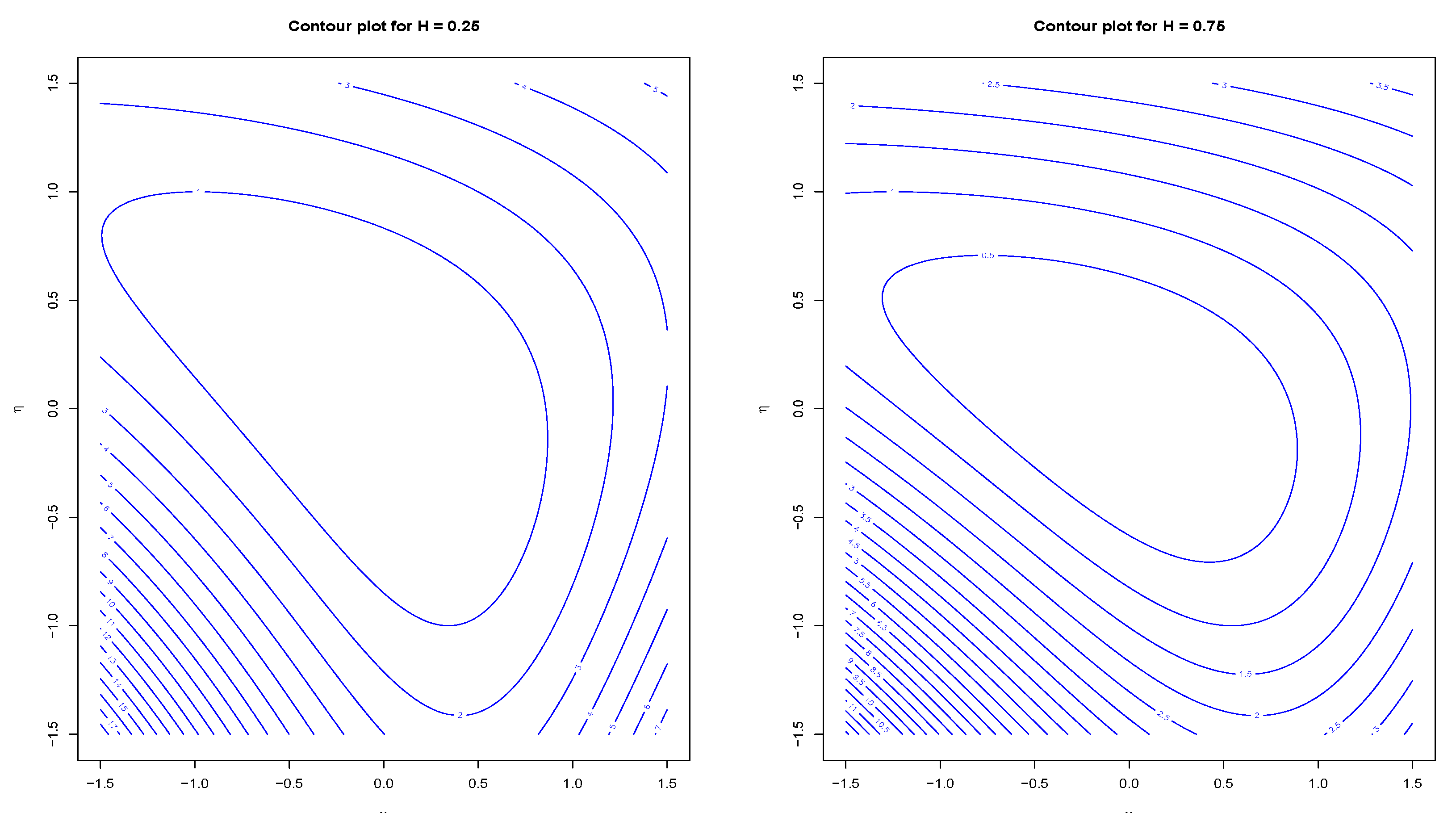
The plots in Figure 1 shows graphically the uniqueness of the minimal point ${\eta }_{*}$ for $H=\frac{1}{4}$ and $H=\frac{3}{4}$. In these particular examples, the contours are convex in the half plane $x>k$, which corresponds to the out-of-money calls. For out-of-money puts, $x<k$, though the contours are not convex, the uniqueness of ${\eta }_{*}$ sustains.

So long as we establish an asymptotic for the log price $lnC(k,t)$ for $k>x_0$, by using the following small time asymptotic for implied volatility in Gao and Lee (2014) or Roper and Rutkowski (2009)

$${\sigma }_{\mathrm{BS}}(k,t)=\frac{|k-x_0|}{\sqrt{2t|lnC(k,t\left)\right|}}+O\left(\frac{ln|lnC(k,t\left)\right|}{\sqrt{t}{|lnC(k,t)|}^{3/2}}\right),$$

(19)

an asymptotic formula for implied volatility follows immediately. We summarize the result in the following theorem but omitting its proof.

Theorem 3.

Let $H\le \frac{1}{2}$ and let $k=lnK$ be the log moneyness and $\alpha =\frac{1}{2}-H$. The implied volatility ${\sigma }_{\mathrm{BS}}(k,t)$ for out-of-money calls ($k>x_0$) has the following asymptotic in small time to expiry

$${\sigma }_{\mathrm{BS}}^2(k,t)={\sigma }_{\mathrm{BS}}^2\left(\frac{k}{t^{\alpha }}\right)\approx \frac{{(k-x_0)}^2}{t^{2\alpha }}{\left\{\frac{{\eta }_{*}^2}{{\nu }^2}+\frac{1}{y_0^2\psi \left({\eta }_{*}\right)}{\left(\frac{k-x_0}{t^{\alpha }}-\rho y_0^2{C}_{RK}\left({\eta }_{*}\right)\frac{{\eta }_{*}}{\nu }\right)}^2\right\}}^{-1}.$$

(20)

The minimal point ${\eta }_{*}$ is given Lemma in 2.

Remark 5.

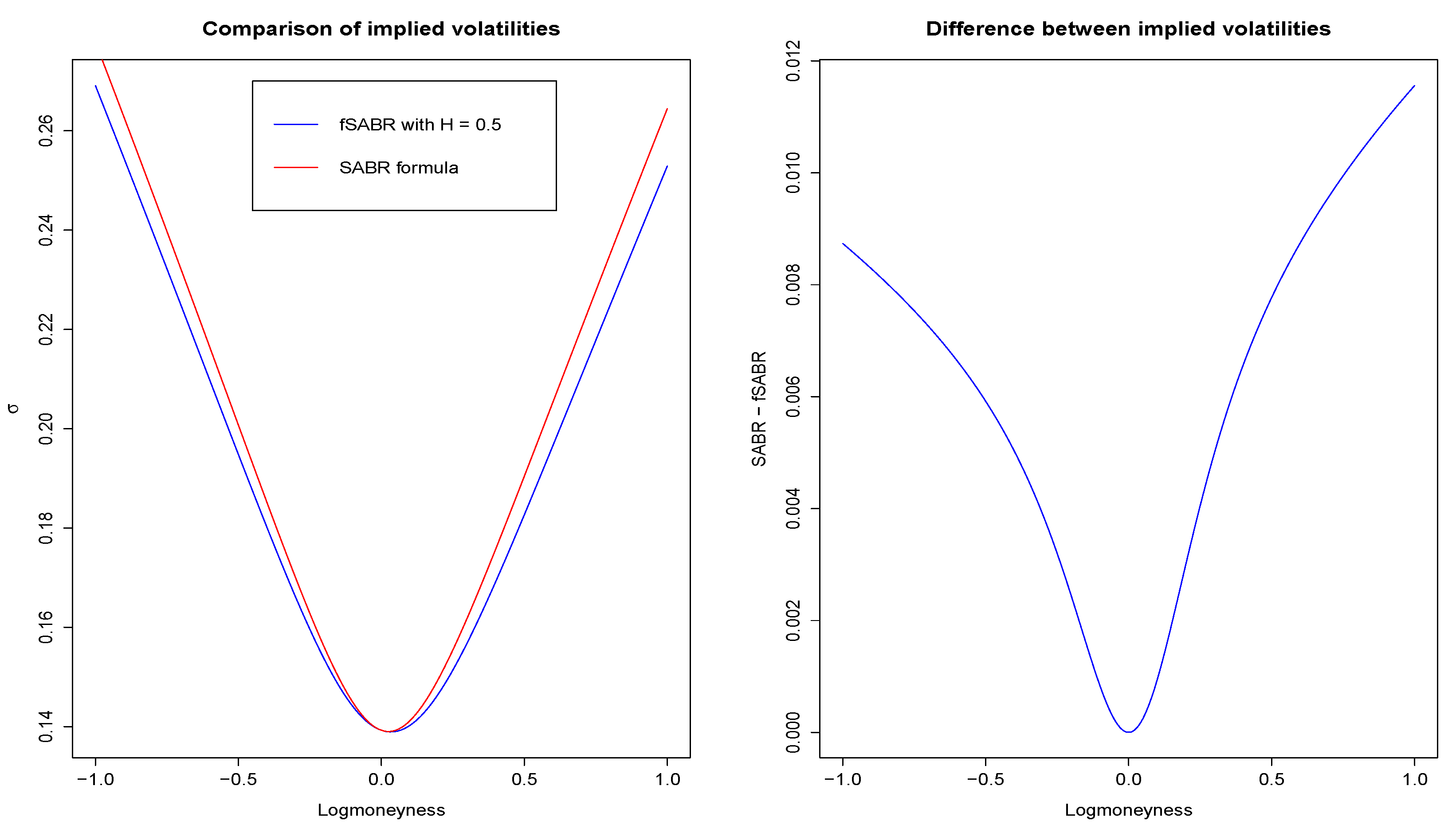
Note that (20) does not recover the SABR formula when $H=\frac{1}{2}$. The derivation of the SABR formula relies heavily on the geometry and symmetry of the underlying SABR plane which is isometric to the Poincaré plane. Figure 2 shows the comparison between the two formulas with time to expiry $t=1$. Parameters are chosen so as to reproduce the figures in Hagan et al. (2002). In this set of parameters, the maximal difference between the two approximate implied volatility curves is about 1% for logmoneyness $k\in [-1,1]$.

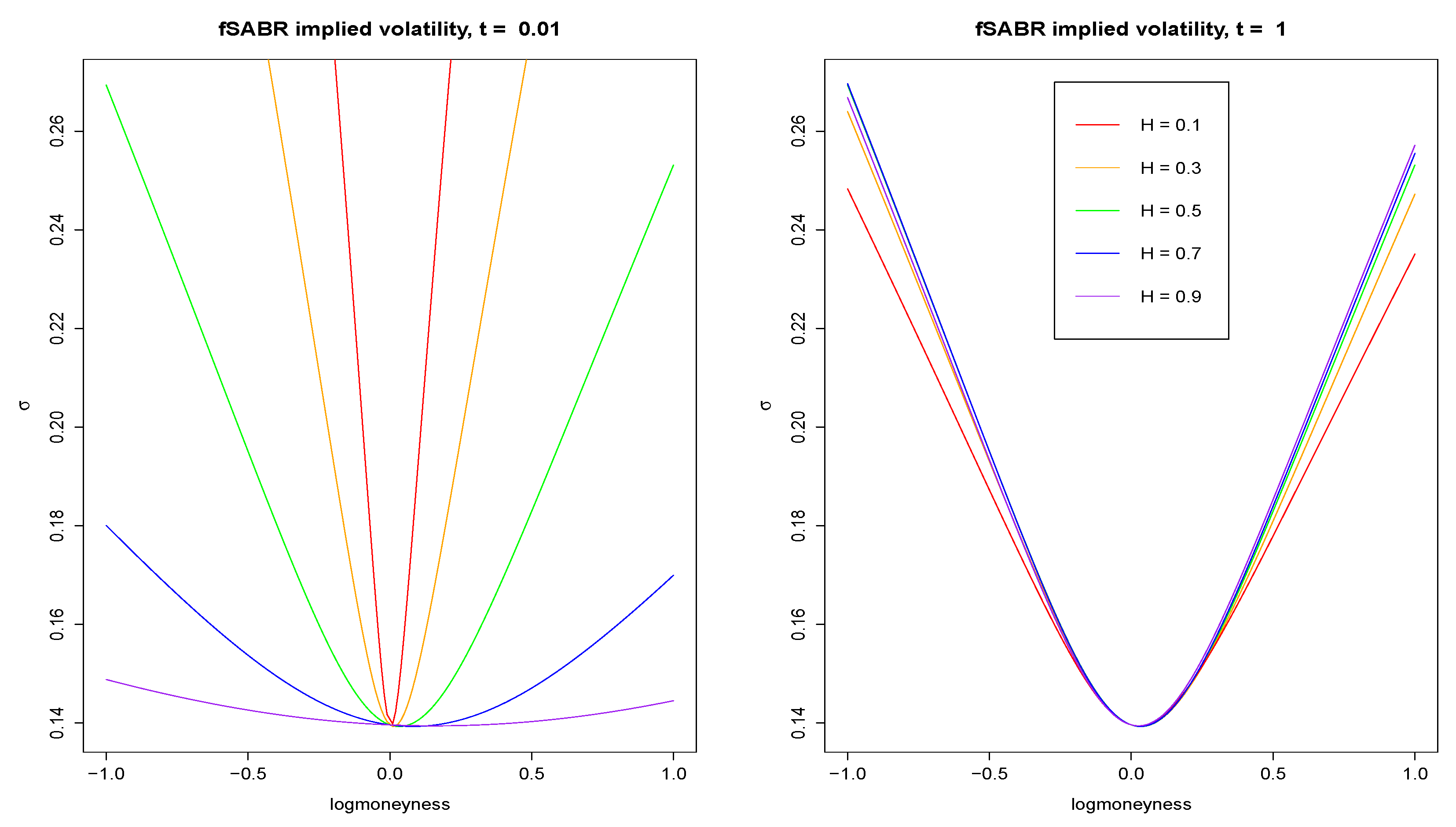
We conclude the section by remarking that, as time to expiry t approaches zero, the approximate implied volatility ${\sigma }_{\mathrm{BS}}(k,t)$ flattens out with $H>\frac{1}{2}$; whereas the whole surface ${\sigma }_{\mathrm{BS}}(k,t)$ explodes with $H<\frac{1}{2}$ except for the at-the-money option $k=x_0$. Figure 3 shows the plots of approximate implied volatilities $\sigma$ given in (20) versus logmoneyness k for time to expiry $t=0.01$ and $t=1$ respectively, and various Hurst exponents H. As in Figure 2, parameters are chosen as $a_0=0.13927$, $\nu =0.5778$, and $\rho =-0.06867$. The numerical determination of the ${\eta }_{*}$’s is relatively efficient since it is basically a one-dimensional optimization problem.

5. A Heuristic Large Deviation Principle

In this section, we provide a heuristic derivation of the sample path large deviation principle for $(X_t,Y_t)$ in small time by bootstrapping the bridge representation to multiperiod. For simplicity, we introduce the following vector notations.

$$\begin{array}{ccc}& & \mathit{t}=(t_1,\dots ,t_n),{\mathit{x}}_{\mathit{t}}=(x_{t_1},\dots ,x_{t_n}),{\mathit{y}}_{\mathit{t}}=(y_{t_1},\dots ,y_{t_n}),\hfill \\ & & {\mathit{B}}_{\mathit{t}}^H=(B_{t_1}^H,\dots ,B_{t_n}^H),{\mathit{X}}_{\mathit{t}}=(X_{t_1},\dots ,X_{t_n}),{\mathit{Y}}_{\mathit{t}}=(Y_{t_1},\dots ,Y_{t_n}),\hfill \\ & & {\xi }_{\mathit{t}}=({\xi }_{t_1},\dots ,{\xi }_{t_n}),{\eta }_{\mathit{t}}=({\eta }_{t_1},\dots ,{\eta }_{t_n}),{\zeta }_{\mathit{t}}=({\zeta }_{t_1},\dots ,{\zeta }_{t_n}).\hfill \end{array}$$

Theorem 4.

The multiperiod joint density p of $(X_t,Y_t)$

$$\begin{array}{ccc}& & p(x_1,y_1,\dots ,x_n,y_n):=\mathbb{P}\left[(X_{t_1},Y_{t_1})=(x_1,y_1),\dots ,(X_{t_n},Y_{t_n})=(x_n,y_n)\right]\hfill \end{array}$$

has the following bridge representation

$$\begin{array}{ccc}& & p(x_1,y_1,\dots ,x_n,y_n)\hfill \\ & =& \mathbb{E}\left[\left.\prod _{k=1}^n\frac{1}{\sqrt{2\pi y_0^2{\overline{\rho }}^2\Delta v_{t_k}}}{e}^{-\frac{1}{2y_0^2{\overline{\rho }}^2\Delta v_{t_k}}{\left(\Delta x_{t_k}-y_0\rho {\int }_{t_{k-1}}^{t_k}{e}^{\nu B_s^H}d{B}_s+\frac{y_0^2}{2}\Delta v_{t_k}\right)}^2}\right|\nu {\mathit{B}}_{\mathit{t}}^H={\eta }_{\mathit{t}}\right]\times \hfill \\ & & \mathbb{P}\left[y_0{e}^{\nu {\mathit{B}}_{\mathit{t}}^H}={\mathit{y}}_{\mathit{t}}\right],\hfill \end{array}$$

(21)

where ${\eta }_{\mathit{t}}=log{\mathit{y}}_{\mathit{t}}-log{y}_0$, $\Delta x_{t_k}=x_{t_k}-x_{t_{k-1}}$, and $\Delta v_{t_k}=v_{t_k}-v_{t_{k-1}}$ for $k=1,\dots ,n$. Recall that $v_t={\int }_0^t{e}^{\nu B_s^H}ds$.

Proof. 

For any bounded measurable function $f:{\mathbb{R}}^n\times {\mathbb{R}}^n\to \mathbb{R}$, consider the expectation

$$\begin{array}{ccc}& & \int \int f({\mathit{x}}_{\mathit{t}},{\mathit{y}}_{\mathit{t}})p({\mathit{x}}_{\mathit{t}},{\mathit{y}}_{\mathit{t}})d{\mathit{x}}_{\mathit{t}}d{\mathit{y}}_{\mathit{t}}\hfill \\ & =& \mathbb{E}\left[f({\mathit{X}}_{\mathit{t}},{\mathit{Y}}_{\mathit{t}})\right]\hfill \\ & =& \mathbb{E}\left[\mathbb{E}\left[\left.f({\mathit{X}}_{\mathit{t}},{\mathit{Y}}_{\mathit{t}})\right|{\mathcal{F}}_{t_n}^B\right]\right].\hfill \end{array}$$

Let ${\xi }_{t_i}={\int }_0^{t_i}{e}^{\nu B_s^H}d{W}_s$, ${\zeta }_{t_i}={\int }_0^{t_i}{e}^{\nu B_s^H}d{B}_s$ and thus accordingly $\Delta {\xi }_{t_i}={\xi }_{t_i}-{\xi }_{t_{i-1}}={\int }_{t_{i-1}}^{t_i}{e}^{\nu B_s^H}d{W}_s$, $\Delta {\zeta }_{t_i}={\zeta }_{t_i}-{\zeta }_{t_{i-1}}={\int }_{t_{i-1}}^{t_i}{e}^{\nu B_s^H}d{B}_s$. Note that, conditioned on ${\mathcal{F}}_{t_n}^B$, the random variables $\Delta {\xi }_{t_i}$’s are independent normal with mean 0 and variance $\Delta v_{t_i}$. We calculate the conditional expectation as follows.

$$\begin{array}{ccc}& & \mathbb{E}\left[\left.f({\mathit{X}}_{\mathit{t}},{\mathit{Y}}_{\mathit{t}})\right|{\mathcal{F}}_{t_n}^B\right]\hfill \\ & =& \mathbb{E}\left[\left.f\left(x_0+\rho y_0{\zeta }_{\mathit{t}}-\frac{y_0^2}{2}{\mathit{v}}_{\mathit{t}}+\overline{\rho }{y}_0{\xi }_{\mathit{t}},y_0{e}^{\nu {\mathit{B}}_{\mathit{t}}^H}\right)\right|{\mathcal{F}}_{t_n}^B\right]\hfill \\ & =& \int f\left(x_0+\rho y_0{\zeta }_{\mathit{t}}-\frac{y_0^2}{2}{\mathit{v}}_{\mathit{t}}+\overline{\rho }{y}_0{\xi }_{\mathit{t}},y_0{e}^{\nu {\mathit{B}}_{\mathit{t}}^H}\right)\prod _{k=1}^n\frac{1}{\sqrt{2\pi \Delta v_{t_k}}}{e}^{-\frac{{(\Delta {\xi }_{t_k})}^2}{2\Delta v_{t_k}}}d\Delta {\xi }_{\mathit{t}}.\hfill \end{array}$$

(22)

By applying the change of variables

$$\begin{array}{ccc}& & x_{t_k}=x_0+\rho y_0{\zeta }_{t_k}-\frac{y_0^2}{2}{v}_{t_k}+\overline{\rho }{y}_0{\xi }_{t_k},\hfill \end{array}$$

thus

$$\begin{array}{ccc}& & \Delta {\xi }_{t_k}=\frac{1}{\overline{\rho }{y}_0}\left(\Delta x_{t_k}-\Delta {\zeta }_{t_k}-\frac{y_0^2}{2}\Delta v_{t_k}\right).\hfill \end{array}$$

The integral (22) becomes

$$\begin{array}{ccc}& & \int f\left({\mathit{x}}_{\mathit{t}},y_0{e}^{\nu {\mathit{B}}_{\mathit{t}}^H}\right)\prod _{k=1}^n\frac{1}{\sqrt{2\pi \Delta v_{t_k}}}{e}^{-\frac{{(\Delta {\xi }_{t_k})}^2}{2\Delta v_{t_k}}}d\Delta {\xi }_{\mathit{t}}\hfill \\ & =& \int f\left({\mathit{x}}_{\mathit{t}},y_0{e}^{\nu {\mathit{B}}_{\mathit{t}}^H}\right)\prod _{k=1}^n\frac{1}{\sqrt{2\pi {\overline{\rho }}^2{y}_0^2\Delta v_{t_k}}}{e}^{-\frac{1}{2\overline{\rho }{y}_0\Delta v_{t_k}}{\left(\Delta x_{t_k}-\rho y_0{\int }_{t_{k-1}}^{t_k}{e}^{\nu B_s^H}d{B}_s-\frac{y_0^2}{2}\Delta v_{t_k}\right)}^2}d\Delta {\mathit{x}}_{\mathit{t}}\hfill \\ & =& \int f\left({\mathit{x}}_{\mathit{t}},y_0{e}^{\nu {\mathit{B}}_{\mathit{t}}^H}\right)\prod _{k=1}^n\frac{1}{\sqrt{2\pi {\overline{\rho }}^2{y}_0^2\Delta v_{t_k}}}{e}^{-\frac{1}{2\overline{\rho }{y}_0\Delta v_{t_k}}{\left(\Delta x_{t_k}-\rho y_0{\int }_{t_{k-1}}^{t_k}{e}^{\nu B_s^H}d{B}_s-\frac{y_0^2}{2}\Delta v_{t_k}\right)}^2}d{\mathit{x}}_{\mathit{t}}\hfill \end{array}$$

since the Jacobian between $d\Delta {\mathit{x}}_{\mathit{t}}$ and $d{\mathit{x}}_{\mathit{t}}$ 1. It follows that

$$\begin{array}{ccc}& & \int \int f({\mathit{x}}_{\mathit{t}},{\mathit{y}}_{\mathit{t}})p({\mathit{x}}_{\mathit{t}},{\mathit{y}}_{\mathit{t}})d{\mathit{x}}_{\mathit{t}}d{\mathit{y}}_{\mathit{t}}\hfill \\ & =& \mathbb{E}\left[\left.\mathbb{E}\left[f({\mathit{X}}_{\mathit{t}},{\mathit{Y}}_{\mathit{t}})\right|{\mathcal{F}}_t^B\right]\right]\hfill \\ & =& \mathbb{E}\left[\int f\left({\mathit{x}}_{\mathit{t}},y_0{e}^{\nu {\mathit{B}}_{\mathit{t}}^H}\right)\prod _{k=1}^n\frac{1}{\sqrt{2\pi {\overline{\rho }}^2{y}_0^2\Delta v_{t_k}}}{e}^{-\frac{1}{2\overline{\rho }{y}_0\Delta v_{t_k}}{\left(\Delta x_{t_k}-\rho y_0{\int }_{t_{k-1}}^{t_k}{e}^{\nu B_s^H}d{B}_s-\frac{y_0^2}{2}\Delta v_{t_k}\right)}^2}d{\mathit{x}}_{\mathit{t}}\right]\hfill \\ & =& \int \int d{\mathit{x}}_{\mathit{t}}d{\mathit{y}}_{\mathit{t}}f\left({\mathit{x}}_{\mathit{t}},{\mathit{y}}_{\mathit{t}}\right)\times \hfill \\ & & \mathbb{E}\left[\left.\prod _{k=1}^n\frac{1}{\sqrt{2\pi {\overline{\rho }}^2{y}_0^2\Delta v_{t_k}}}{e}^{-\frac{1}{2\overline{\rho }{y}_0\Delta v_{t_k}}{\left(\Delta x_{t_k}-\rho y_0{\int }_{t_{k-1}}^{t_k}{e}^{\nu B_s^H}d{B}_s-\frac{y_0^2}{2}\Delta v_{t_k}\right)}^2}\right|\nu {\mathit{B}}_{\mathit{t}}^H={\eta }_{\mathit{t}}\right]\times \hfill \\ & & \mathbb{P}\left[y_0{e}^{\nu {\mathit{B}}_{\mathit{t}}^H}={\mathit{y}}_{\mathit{t}}\right].\hfill \end{array}$$

This completes the proof of bridge representation (21) since f is arbitrary.  □

To move onto a heuristic derivation of the sample path large deviation principle for $(X_t,Y_t)$ in small time, we take logarithm on both sides of (21) and obtain

$$\begin{array}{ccc}& & logp(x_{t_1},y_{t_1},\dots ,x_{t_n},y_{t_n})\hfill \\ & =& log\mathbb{E}\left[\left.\prod _{k=1}^n\frac{1}{\sqrt{2\pi y_0^2{\overline{\rho }}^2\Delta v_{t_k}}}{e}^{-\frac{1}{2y_0^2{\overline{\rho }}^2\Delta v_{t_k}}{\left(\Delta x_{t_k}-y_0\rho {\int }_{t_{k-1}}^{t_k}{e}^{\nu B_s^H}d{B}_s+\frac{y_0^2}{2}\Delta v_{t_k}\right)}^2}\right|\nu {\mathit{B}}_{\mathit{t}}^H=\eta \right]\hfill \\ & & +log\mathbb{P}\left[\nu {\mathit{B}}_{\mathit{t}}^H={\eta }_{\mathit{t}}\right]-\sum log{y}_{t_i}.\hfill \end{array}$$

(23)

In the following, we ignore the last term on the right-hand side of (23) and intuitively calculate the limits as $n\to \infty$ of the first two terms. Note that to the leading order we have

$$\begin{array}{ccc}& & log\mathbb{P}\left[\nu {\mathit{B}}_{\mathit{t}}^H={\eta }_{\mathit{t}}\right]\approx -\frac{1}{2{\nu }^2}{\eta }^{\prime }{\mathit{R}}^{-1}\eta ,\hfill \end{array}$$

where $\mathit{R}=\left[R(t_i,t_j)\right]$ is the covariance matrix of ${\mathit{B}}_{\mathit{t}}^H$. We further discretize the autovariance R of fractional Brownian motion as

$$\begin{array}{ccc}& & R(t_i,t_j)=\mathbb{E}\left[B_{t_i}^H{B}_{t_i}^H\right]={\int }_0^{t_i\wedge t_j}{K}_H(t_i,s)K_H(t_j,s)ds\hfill \\ & \approx & \sum _{k=0}^{i\wedge j}{K}_H(t_i,t_k)K_H(t_j,t_k)\Delta t={\mathit{K}}^{\prime }\mathit{K}\Delta t,\hfill \end{array}$$

where $\mathit{K}$ denotes the upper triangular matrix

$${\mathit{K}}_{ij}=\left\{\begin{array}{cc}{K}_H(t_i,t_j),\hfill & \mathrm{if} i\ge j;\hfill \\ & \\ 0,\hfill & \mathrm{otherwise}.\hfill \end{array}\right.$$

Thereby, ${\mathit{R}}^{-1}=\frac{1}{\Delta t}{\mathit{K}}^{-1}{\left({\mathit{K}}^{\prime }\right)}^{-1}$. Let $\mathit{b}=(b_{t_1},\dots b_{t_n})$ be the solution to the linear system

$$\frac{\eta }{\nu }=\mathit{K}\mathit{b}\Delta t.$$

It follows that

$$\begin{array}{ccc}& & \frac{1}{2{\nu }^2}{\eta }^{\prime }{\mathit{R}}^{-1}\eta =\frac{1}{2}\Delta t{\mathit{b}}^{\prime }{\mathit{K}}^{\prime }{\mathit{R}}^{-1}\mathit{K}\mathit{b}\Delta t\hfill \\ & =& \frac{1}{2}{\mathit{b}}^{\prime }\mathit{b}\Delta t=\frac{1}{2}\sum _{k=1}^n{b}_{t_k}^2\Delta t\hfill \\ & ⟶& \frac{1}{2}{\int }_0^T{b}_t^{2}dtasn\to \infty .\hfill \end{array}$$

Also in the limit as $n\to \infty$, we obtain ${\eta }_t=\nu {\int }_0^t{K}_H(t,s)b_{s}ds$.

On the other hand, for the first term on the right-hand side of (23), we have

$$\begin{array}{ccc}& & log\mathbb{E}\left[\left.\prod _{k=1}^n\frac{1}{\sqrt{2\pi y_0^2{\overline{\rho }}^2\Delta v_{t_k}}}{e}^{-\frac{1}{2y_0^2{\overline{\rho }}^2\Delta v_{t_k}}{\left(\Delta x_{t_k}-y_0\rho {\int }_{t_{k-1}}^{t_k}{e}^{\nu B_s^H}d{B}_s+\frac{y_0^2}{2}\Delta v_{t_k}\right)}^2}\right|\nu {\mathit{B}}^H=\eta \right]\hfill \\ & \approx & \sum _{k=1}^n\mathbb{E}\left[\left.-\frac{1}{2y_0^2{\overline{\rho }}^2\Delta v_{t_k}}{\left(\Delta x_{t_k}-y_0\rho {\int }_{t_{k-1}}^{t_k}{e}^{\nu B_s^H}d{B}_s\right)}^2\right|\nu {\mathit{B}}^H=\eta \right].\hfill \end{array}$$

Note that conditioned on $\nu {\mathit{B}}^H=\eta$, we have

$$\begin{array}{ccc}& & \Delta v_{t_k}={\int }_{t_{k-1}}^{t_k}{e}^{2\nu B_s^H}ds\approx e^{2{\eta }_{t_{k-1}}}\Delta t=e^{2\nu {\sum }_{j=0}^{k-1}{K}_H(t_{k-1},t_j)b_{t_j}\Delta t}\Delta t\hfill \end{array}$$

as well as

$$\begin{array}{ccc}& & \Delta x_{t_k}-y_0\rho {\int }_{t_{k-1}}^{t_k}{e}^{\nu B_s^H}d{B}_s\approx \Delta x_{t_k}-y_0\rho e^{{\eta }_{t_{k-1}}}{b}_{t_{k-1}}\Delta t\hfill \\ & =& \left(\frac{\Delta x_{t_k}}{\Delta t}-y_0\rho e^{\nu {\sum }_{j=0}^{k-1}{K}_H(t_{k-1},t_j)b_{t_j}\Delta t}{b}_{t_{k-1}}\right)\Delta t.\hfill \end{array}$$

It follows that the first term in (23) has the limit

$$\begin{array}{ccc}& & \sum _{k=1}^n\mathbb{E}\left[\left.-\frac{1}{2y_0^2{\overline{\rho }}^2\Delta v_{t_k}}{\left(\Delta x_{t_k}-y_0\rho {\int }_{t_{k-1}}^{t_k}{e}^{\nu B_s^H}d{B}_s\right)}^2\right|\nu {\mathit{B}}^H=\eta \right]\hfill \\ & \approx & -\sum _{k=0}^n\frac{1}{2y_0^2{\overline{\rho }}^2{e}^{2\nu {\sum }_{j=0}^{k-1}{K}_H(t_{k-1},t_j)b_{t_j}\Delta t}}{\left(\frac{\Delta x_{t_k}}{\Delta t}-y_0\rho e^{\nu {\sum }_{j=0}^{k-1}{K}_H(t_{k-1},t_j)b_{t_j}\Delta t}{b}_{t_{k-1}}\right)}^2\Delta t\hfill \\ & ⟶& -\frac{1}{2}{\int }_0^T\frac{1}{y_0^2{\overline{\rho }}^2{e}^{2\nu {\int }_0^t{K}_H(t,s)b_{s}ds}}{\left({\dot{x}}_t-y_0\rho e^{\nu {\int }_0^t{K}_H(t,s)b_{s}ds}{b}_t\right)}^{2}dt\hfill \end{array}$$

as $n\to \infty$.

Putting the two limits together, we obtain heuristically for $T\approx 0$ that

$$\begin{array}{ccc}& & -log\mathbb{P}\left[X_t=x_t,Y_t=y_t,fort\in [0,T]\right]\hfill \\ & \approx & \frac{1}{2}{\int }_0^T\frac{1}{y_0^2{\overline{\rho }}^2{e}^{2\nu {\int }_0^t{K}_H(t,s)b_{s}ds}}{\left({\dot{x}}_t-y_0\rho e^{\nu {\int }_0^t{K}_H(t,s)b_{s}ds}{b}_t\right)}^{2}dt+\frac{1}{2}{\int }_0^T{b}_t^{2}dt\hfill \\ & =& \frac{1}{2}{\int }_0^T\frac{1}{{\overline{\rho }}^2{y}_t^2}{\left({\dot{x}}_t-\rho y_t{b}_t\right)}^{2}dt+\frac{1}{2}{\int }_0^T{b}_t^{2}dt\hfill \\ & =& \frac{1}{2}{\int }_0^T\frac{1}{{\overline{\rho }}^2}{\left(\frac{{\dot{x}}_t}{y_t}-\rho b_t\right)}^{2}dt+\frac{1}{2}{\int }_0^T{b}_t^{2}dt,\hfill \end{array}$$

(24)

where $b\in L^2[0,T]$ satisfies the integral equation

$$log{y}_t-log{y}_0=\nu {\int }_0^t{K}_H(t,s)b_{s}ds$$

for all $t\in [0,T]$. We remark that (24) should serve as the rate function for the sample path large deviation principle in small time for $(X_t,Y_t)$. Moreover, one may define the “geodesic” from the initial point $(x_0,y_0)$ to the terminal point $(x_T,y_T)$ in the fSABR plane as the path $(x_t^{*},y_t^{*})$ which minimizes the functional (24), i.e.,

$$\begin{array}{c}\hfill (x_t^{*},y_t^{*}):=\underset{t\mapsto (x_t,y_t)}{\mathrm{argmin}}\frac{1}{2}{\int }_0^T\frac{1}{{\overline{\rho }}^2}{\left(\frac{{\dot{x}}_t}{y_t}-\rho b_t\right)}^{2}dt+\frac{1}{2}{\int }_0^T{b}_t^{2}dt,\end{array}$$

where again $b_t$ is determined by solving the integral equation

$$log{y}_t-log{y}_0=\nu {\int }_0^t{K}_H(t,s)b_{s}ds.$$

(25)

Also, the minimizer can be regarded as the “geodesic” connecting $(x_0,y_0)$ and $(x_T,y_T)$.

Remark 6.

Note that $b_t$ is indeed determined by the inverse operator $K_H^{-1}$ applied to $log\frac{y_t}{y_0}$. In particular, with $H=\frac{1}{2}$ this inverse operator reduces to the usual derivative. Thus, with $H=\frac{1}{2}$,

$$b_t=\frac{d}{dt}\left(log\frac{y_t}{y_0}\right)=\frac{{\dot{y}}_t}{y_t}.$$

The functional (24) becomes

$$\begin{array}{ccc}& & \frac{1}{2}{\int }_0^T\frac{1}{{\overline{\rho }}^2}{\left(\frac{{\dot{x}}_t}{y_t}-\rho b_t\right)}^{2}dt+\frac{1}{2}{\int }_0^T{b}_t^{2}dt\hfill \\ & =& \frac{1}{2}{\int }_0^T\frac{1}{{\overline{\rho }}^2}{\left(\frac{{\dot{x}}_t}{y_t}-\rho \frac{{\dot{y}}_t}{y_t}\right)}^{2}dt+\frac{1}{2}{\int }_0^T\frac{{\dot{y}}_t^2}{y_t^2}dt\hfill \\ & =& \frac{1}{2}{\int }_0^T\frac{1}{{\overline{\rho }}^2{y}_t^2}\left({\dot{x}}_t^2-2\rho {\dot{x}}_t{\dot{y}}_t+{\dot{y}}_t^2\right)dt.\hfill \end{array}$$

The last expression is the energy functional (up to the constant factor $\frac{1}{2}$) associated with the Riemann metric $d{s}^2=\frac{1}{{\overline{\rho }}^2{y}^2}(d{x}^2-2\rho dxdy+d{y}^2)$. The diffusion process associated with this Riemann metric is governed by the SDEs

$$\begin{array}{ccc}& & d{X}_t=Y_{t}d{W}_t,\hfill \\ & & d{Y}_t=Y_{t}d{Z}_t,\hfill \end{array}$$

where $W_t$ and $Z_t$ are correlated Brownian motion with constant correlation ρ, which up to a linear transformation is the upper plane model of the Poincaré space. In other words, with $H=\frac{1}{2}$, the functional (24) recovers the energy functional for the classical Poincaré space, which is isometric to the SABR plane.

Lastly, with the aid of the sample path large deviation principle (24), it is nearly a common practice, say by applying the Laplace asymptotic formula, to conclude that the log premium of an out-of-money call in small time has the asymptotic as $t\to 0$

$$-logC(k,t)\approx -log\mathbb{P}\left[X_t\ge k\right]\approx \frac{1}{2}{\int }_0^T\frac{1}{{\overline{\rho }}^2}{\left(\frac{{\dot{x}}_t^{*}}{y_t^{*}}-\rho b_t^{*}\right)}^{2}dt+\frac{1}{2}{\int }_0^T{b_t^{*}}^{2}dt,$$

where $(x_t^{*},y_t^{*},b_t^{*})$ denotes the optimal path that minimizes the functional (24) subject to the constraint $x_t^{*}=k$ and $y_t^{*}$, $b_t^{*}$ satisfy the integral Equation (25). Thus, by applying (19), an approximation of implied volatility in small time is readily obtained. We summarize the result in the following proposition which, with $H=\frac{1}{2}$, recovers the SABR Formula (3). However, for $H\ne \frac{1}{2}$, the numerical implementation of (26) is more involved than that of (20) since, as opposed to a one dimensional optimization problem, it is subject to solving a two-dimensional constrained variational problem.

Proposition 1

(fSABR formula). Let $k=log\left(\frac{K}{s_0}\right)$ be the log moneyness. The implied volatility ${\sigma }_{\mathrm{BS}}(k,t)$ in a small time to expiry has the asymptotics

$${\sigma }_{\mathrm{BS}}^2\approx \frac{k^2}{T}{\left({\int }_0^T\left\{\frac{1}{{\overline{\rho }}^2{y_t^{*}}^2}{\left({\dot{x}}_t^{*}-\rho y_t^{*}{b}_t^{*}\right)}^2+{b_t^{*}}^2\right\}dt\right)}^{-1},$$

(26)

where $(x_t^{*},b^{*})$ is the minimizer of the variational problem

$$(x^{*},b^{*})=argmin\left\{\dot{x},b\in L^2[0,T]:{\int }_0^T\left(\frac{1}{{\overline{\rho }}^2{y}_t^2}{\left({\dot{x}}_t-\rho y_t{b}_t\right)}^2+b_t^2\right)dt\right\}$$

with $x_T=k$ and $y_t^{*}$ satisfying

$$log{y}_t^{*}-log{y}_0=\nu {\int }_0^t{K}_H(t,s)b_s^{*}ds$$

for $t\in [0,T]$. Notice that (26) recovers the SABR Formula (3) with $H=\frac{1}{2}$.

6. Conclusions and Discussion

We showed in this paper a bridge representation in Fourier space and a small time asymptotic for the joint probability of lognormal fractional SABR model for general $\rho \in (-1,1)$. An application of the asymptotics of the joint density is an approximation of the implied volatility in a short time. Due to the different nature of methodologies, the newly obtained approximation of implied volatilities in small time does not recover the celebrated SABR formula for implied volatility (to the zeroth order) when the Hurst exponent H equals a half. To recover the SABR formula, we presented a heuristic derivation of the sample path large deviation principle for the lognormal fractional SABR model by bootstrapping via the multiperiod joint density. We emphasize once again that the same trick is applicable to general fractional SABR models, i.e., to include a local volatility component in the process $S_t$ for an underlying asset. We leave the rigorous proof of the sample path large deviation principle for fractional SABR models in future work. Lastly, the bridge representation methodology is also applicable to the case in which the volatility process is governed by an exponential fractional Ornstein-Uhlenbeck process since a fractional Ornstein-Uhlenbeck process is Gaussian as well. However, as the time to expiry approaches zero, the mean reversion part does not really play a role in the large deviation regime.

References

1. Baillie, Richard T., Tim Bollerslev, and Hans Ole Mikkelsen. 1996. Fractionally integrated generalized autoregressive conditional heteroskedasticity. Journal of Econometrics 74: 3–30. [Google Scholar] [CrossRef]
2. Cheng, Xue, and Tai-Ho Wang. 2018. Bessel bridge representation for heat kernel in hyperbolic space. Proceedings of the American Mathematical Society 146: 1781–92. [Google Scholar] [CrossRef]
3. Comte, Fabienne, and Eric Renault. 1998. Long memory in continuous-time stochastic volatility models. Mathematical Finance 8: 291–323. [Google Scholar] [CrossRef]
4. Comte, Fabienne, Laure Coutin, and Eric Renault. 2012. Affine fractional stochastic volatility models. Annals of Finance 8: 337–78. [Google Scholar] [CrossRef]
5. Cont, Rama, and Purba Das. 2022. Rough Volatility: Fact or Artifact? arXiv arXiv:2203.13820. [Google Scholar]
6. Decreusefond, Laurent, and A. Suleyman Üstünel. 1999. Stochastic analysis of the fractional Brownian motion. Potential Analysis 10: 177–214. [Google Scholar] [CrossRef]
7. Ekström, Erik, and Bing Lu. 2015. Short-time implied volatility in exponential Lévy models. International Journal of Theoretical and Applied Finance 18: 1550025. [Google Scholar] [CrossRef] [Green Version]
8. El Euch, Omar, and Mathieu Rosenbaum. 2019. The characteristic function of rough Heston models. Mathematical Finance 29: 3–38. [Google Scholar] [CrossRef] [Green Version]
9. Gao, Kun, and Roger Lee. 2014. Asymptotics of implied volatility to arbitrary order. Finance and Stochastics 18: 349–92. [Google Scholar] [CrossRef]
10. Gatheral, Jim, Thibault Jaisson, and Mathieu Rosenbaum. 2018. Volatility is rough. Quantitative Finance 18: 933–49. [Google Scholar] [CrossRef]
11. Granger, Clive W. J., and Roselyne Joyeux. 1980. An introduction to long memory time series models and fractional differencing. Journal of Time Series Analysis 1: 15–39. [Google Scholar] [CrossRef]
12. Guennoun, Hamza, Antoine Jaquier, Patrick Roome, and Fangwei Shi. 2018. Asymptotic behavior of the fractional Heston model. SIAM Journal on Financial Mathematics 9: 337–78. [Google Scholar] [CrossRef]
13. Hagan, Patrick, Deep Kumar, Andrew Lesniewski, and Diana Woodward. 2002. Managing smile risk. Wilmott Magazine 1: 84–108. [Google Scholar]
14. Hagan, Patrick, Andrew Lesniewski, and Diana Woodward. 2015. Probability distribution in the SABR Model of stochastic volatility. In Large Deviations and Asymptotic Methods in Finance. Springer Proceedings in Mathematics & Statistics. Cham: Springer, vol. 110, pp. 1–35. [Google Scholar]
15. Hu, Yaozhong. 2017. Analysis on Gaussian Space. Singapore: World Scientific. [Google Scholar]
16. Ikeda, Nobuyuki, and Hiroyuki Matsumoto. 1999. Brownian Motion on the Hyperbolic Plane and Selberg Trace Formula. Journal of Functional Analysis 163: 63–100. [Google Scholar] [CrossRef] [Green Version]
17. Jarrow, Robert A., Philip Protter, and Hasanjan Sayit. 2009. No arbitrage without semimartingales. The Annals of Applied Probability 19: 596–616. [Google Scholar] [CrossRef]
18. Mishura, Yuliya. 2008. Stochastic Calculus for Fractional Brownian Motion and Related Processes. Lecture Notes in Mathematics. Berlin and Heidelberg: Springer Science & Business Media, vol. 1929. [Google Scholar]
19. Nualart, David. 2006. The Malliavin Calculus and Related Topics, 2nd ed. Berlin and Heidelberg: Springer. [Google Scholar]
20. Rogers, Chris. 2019. Things We Think We Know. Available online: https://www.skokholm.co.uk/wp-content/uploads/2019/11/TWTWKpaper.pdf (accessed on 1 June 2022).
21. Roper, Michael, and Marek Rutkowski. 2009. A note on the behaviour of the Black-Scholes implied volatility close to expiry. International Journal of Theoretical and Applied Finance 12: 427–41. [Google Scholar] [CrossRef]
Figure 1. The contour plots. Parameters ρ = 0.7 , ν = 1 , y 0 = 1 , t = 0.5 . H = 0.75 on the right; H = 0.25 , on the left.
Risks 10 00156 g001
Figure 2. The plot on the left shows the approximate implied volatility curves versus logmoneyness with time to expiry t = 1 produced by (20) (in blue) the SABR Formula (3) (in red). Parameters are set as ρ = 0.06867 , ν = 0.5778 , a 0 = 0.13927 . The plot on the right shows the difference between the two curves.
Risks 10 00156 g002
Figure 3. The implied volatility curves for t = 0.01 on the left, t = 1 on the right. Parameters are set as ρ = 0.06867 , ν = 0.5778 , a 0 = 0.13927 . H = 0.1 in red, H = 0.3 in orange, H = 1 2 in green, H = 0.7 in blue, H = 0.9 in purple.
Risks 10 00156 g003
Publisher’s Note: MDPI stays neutral with regard to jurisdictional claims in published maps and institutional affiliations.