Bivariate Copula Trees for Gross Loss Aggregation with Positively Dependent Risks

Abstract

We propose several numerical algorithms to compute the distribution of gross loss in a positively dependent catastrophe insurance portfolio. Hierarchical risk aggregation is performed using bivariate copula trees. Six common parametric copula families are studied. At every branching node, the distribution of a sum of risks is obtained by discrete copula convolution. This approach is compared to approximation by a weighted average of independent and comonotonic distributions. The weight is a measure of positive dependence through variance of the aggregate risk. During gross loss accumulation, the marginals are distorted by application of insurance financial terms, and the value of the mixing weight is impacted. To accelerate computations, we capture this effect using the ratio of standard deviations of pre-term and post-term risks, followed by covariance scaling. We test the performance of our algorithms using three examples of complex insurance portfolios subject to hurricane and earthquake catastrophes.

1. Introduction

Catastrophe models are widely used by insurers to help weather extreme natural catastrophe events and to ascertain that they are able to manage their risk and pay their claims (Grossi 2004; Grossi et al. 2005). The models estimate how frequent and severe future catastrophes are likely to be, where they are likely to occur and the amount of damage they can inflict. Individual instances of peril, e.g., a simulated earthquake with a particular magnitude, are called events and are typically created using Monte Carlo sampling of model parameters (Clark 2015). Large catalogs of simulated events are generated, representing an ensemble of hypothetical catastrophes in the period of, e.g., 10,000 years. For each event in the catalog, the model calculates the peril’s intensity (e.g., wind speed for hurricanes, degree of ground shaking for earthquakes or water level for floods) at each location within the affected area. Then, the intensity together with information about the type of construction and occupancy for each insured property is converted into a probability distribution of loss using a so-called vulnerability module. Finally, property losses are summed up into the event’s total loss using a loss-aggregation algorithm (Grossi et al. 2005). Insurance contract terms, applicable to the sharing of risk on each property or groups of properties, determine loss perspective on the event total, such as:

• Ground-up loss (total loss without any policy conditions applied)
• Retained loss (loss retained by insured party)
• Gross loss (loss to an insurer after application of policy financial terms)

To investigate the impact of catalog events on a portfolio of properties, the event total losses are further aggregated within each catalog year into an annual loss. Property loss, event total and annual loss are typically modeled as discrete random variables (Cossette et al. 2003) characterized by probability mass functions (pmfs). Finally, the mixture of annual loss pmfs is transformed into the exceedance probability (EP) curve (Grossi et al. 2005). The EP curve helps insurers determine losses that correspond to percentiles of the annual loss for all simulated catalog years.

The basic step in portfolio loss analysis is computation of the event total loss (Cossette et al. 2003; Dhaene et al. 2014; Wang 1998). This procedure can be thought of as estimation of the distribution of the sum $S=X_1+X_2+\dots ,+X_m$ of positively dependent, non-negative random variables $X_1,X_2,\dots ,X_m$ when the joint distribution of these variables is unavailable. Many researchers have studied this problem in the context of Fréchet theory and have shown its application to finance (see, e.g., Deelstra et al. 2011; Kaas et al. 2000; Linders and Stassen 2016). The latter contributions offer closed-form expressions for the upper or lower convex bounds of S when the statistics at hand are restricted to, usually parametric, continuous marginal distributions characterizing $X_1,X_2,\dots ,X_m$ and partial information on the joint dependence structure of the random vector $(X_1,X_2,\dots ,X_m)$. Another line of research addressed the problem of risk aggregation, modeling the joint distribution using copulas. By assuming a parametric form of the marginals and a parametric form of the copula, the probability density function (pdf) of S is derived in closed form (see, e.g., Cossette et al. 2013; Marri and Moutanabbir 2022; Vernic 2016). For high-dimensional portfolios, however, fitting a copula that reproduces the prescribed data statistics proves difficult. Another technical complication is that for some combinations of parametric marginals and parametric copulas, estimation of the pdf of S entails a multivariate convolution integral, which is computationally cumbersome for large portfolios. An avant garde workaround referred to as copula-based hierarchical risk aggregation has been proposed recently (Arbenz et al. 2012; Bruneton 2011; Coté and Genest 2015; Derendinger 2015; Joe and Sang 2016) to alleviate the aforementioned bottlenecks. This approach eliminates the need to parameterize one copula for all the risks as it defines the joint, usually bivariate, dependence between partial sums of risks in the subsequent loss accumulation steps. Such a hierarchical pathway of adding dependent risks is represented as a bivariate aggregation tree with copulas describing summation nodes. The original implementation in Arbenz et al. (2012) uses Monte Carlo sampling. Significantly faster convolution-based implementation has been discussed in our previous contribution on ground-up loss estimation (Wójcik et al. 2019). In the present study, we extend this technique in three ways. First, we adapt it to gross loss computation. Second, apart from using Fréchet copula only, we also consider five other copula families commonly applied in insurance and mathematical finance (see, e.g, Bouyé et al. 2000; Venter 2002). Lastly, we enhance the methodology for risk summation from the previously implemented mixture of classical convolution and numerical quantile addition to discrete copula convolution.

Following, we seek to approximate the pmf $p_{\varphi \left(S\right)}$ of $\varphi \left(S\right)=\varphi (X_1+X_2+,\dots ,X_m)$ where the insurance policy terms $\varphi$ represent nonlinear transformations of partial loss aggregates in hierarchical trees. We assume that the random vector $(X_1,X_2,\dots ,X_m)$ is weakly associated and that the generally nonparametric marginal pmfs of $X_i$ and the non-negative covariance $\mathrm{Cov}[X_i,X_j]$ are known; see Section 2. We analyze gross loss aggregation runs using three insurance portfolios impacted by hurricane and earthquake events. The dependency models cover a broad range of association, shifting focus from correlation between moderately sized losses in the bulk of distributions to correlation between large losses in the upper tails of distributions. We compare the total gross loss pmfs $p_{\varphi \left(S\right)}$ obtained with these models, along with their convex decomposition, in terms of second-order statistics and tail measures of risk. We also provide a detailed discussion of algorithmic implementation of our methods and compare their execution times. We introduce a fast approximation based on Fréchet copula and covariance scaling. For the analyzed portfolios, the latter generates a ∼2–300× speedup compared to the other copulas.

The paper is organized as follows. To start, we provide independent and comonotonic bounds for a gross loss sum of weakly associated risks. Then, we outline a copula-based risk accumulation scheme and discuss the basics of bivariate copulas underlying the summation nodes. Next, we cover the computational aspects of two-stage gross loss accumulation. Lastly, we perform gross loss analysis for two hurricane events and one earthquake event in the United States. Different features of the proposed models are discussed by comparing several risk measures and processing times of aggregation runs.

2. Preliminaries

2.1. Basic Concepts

We start with introducing some notations. A non-negative random variable X with finite expectation and variance is called a risk. For $m\ge 2$ let $\mathbf{X}=(X_1,\dots ,X_m)$ be the portfolio of risks (locations). We assume for any pair of disjoint subsets $A_1,A_2\subseteq \{1,\dots ,m\}$, components of $\mathbf{X}$ are weakly associated:

$$\mathrm{Cov}[\varphi \left(X_i\right),\psi \left(X_j\right)]\ge 0i\in A_1,j\in A_2$$

(1)

for all pairs of nondecreasing functions $\varphi :{\mathbb{R}}^k\to \mathbb{R},\psi :{\mathbb{R}}^{m-k}\to \mathbb{R}$ for $1\le k<m$ such that the above covariance exists (Christofides and Vaggelatou 2004). We denote by ${\mathbf{X}}^{\perp }=(X_1^{\perp },X_2^{\perp },\dots X_m^{\perp })$ and ${\mathbf{X}}^{+}=(X_1^{+},X_2^{+},\dots X_m^{+})$ independent and comonotone random vectors characterized by the same marginals $P_{X_1},P_{X_2},\dots ,P_{X_m}$ as $\mathbf{X}$. By definition, $P_{{\mathbf{X}}^{\perp }}\left(\mathbf{x}\right)=\prod P_{X_i}\left(x_i\right)$ and $P_{{\mathbf{X}}^{+}}\left(\mathbf{x}\right)=min(P_{X_1}\left(x_1\right),P_{X_2}\left(x_2\right),\dots ,P_{X_m}\left(x_m\right))$. Since (1) fulfills the properties of multivariate positive dependence structure (B1–B7 in Colangelo et al. 2005), the following stochastic order holds:

$$P_{{\mathbf{X}}^{\perp }}\left(\mathbf{x}\right)\le P_{\mathbf{X}}\left(\mathbf{x}\right)\le P_{{\mathbf{X}}^{+}}\left(\mathbf{x}\right)\forall \mathbf{x}\in {\mathbb{R}}_{+}^m$$

(2)

Now, let $g:{\mathbb{R}}^m\to \mathbb{R}$ be a supermodular function such that:

$$g(\mathbf{x}\wedge \mathbf{y})+g(\mathbf{x}\vee \mathbf{y})\ge g\left(\mathbf{x}\right)+g\left(\mathbf{y}\right)\forall \mathbf{x},\mathbf{y}$$

(3)

where $\mathbf{x}\wedge \mathbf{y}$ is the componentwise minimum and $\mathbf{x}\vee \mathbf{y}$ the componentwise maximum of $\mathbf{x}$ and $\mathbf{y}$. Christofides and Vaggelatou (2004) show that (1) leads to the following precedence:

$${\mathbf{X}}^{\perp }{\le }_{sm}\mathbf{X}{\le }_{sm}{\mathbf{X}}^{+}$$

(4)

where ${\le }_{sm}$ stands for the supermodular order. Equivalently,

$$\mathrm{E}\left[g\left({\mathbf{X}}^{\perp }\right)\right]\le \mathrm{E}\left[g\left(\mathbf{X}\right)\right]\le \mathrm{E}\left[g\left({\mathbf{X}}^{+}\right)\right]$$

(5)

for all real supermodular functions g, provided that the expectations exist. A few examples of supermodular functions are shown in Figure 1. It follows from Proposition 7 in Cossette et al. (2003) that (4) allows establishment of a convex order relation between the dependent sum $S=X_1+X_2+\dots +X_m$ and its independent $S^{\perp }=X_1^{\perp }+X_2^{\perp }+\dots +X_m^{\perp }$ and comonotone $S^{+}=X_1^{+}+X_2^{+}+\dots +X_m^{+}$ counterparts:

$$S^{\perp }{\le }_{cx}S{\le }_{cx}{S}^{+}$$

(6)

where ${\le }_{cx}$ stands for the convex order defined as:

$$\mathrm{E}\left[v\left(S^{\perp }\right)\right]\le \mathrm{E}\left[v\left(S\right)\right]\le \mathrm{E}\left[v\left(S^{+}\right)\right)]$$

(7)

for all real convex functions $v:\mathbb{R}\to \mathbb{R}$ provided the expectations exist. Equality of expectations $\mathrm{E}\left[S^{\perp }\right]=\mathrm{E}\left[S\right]=\mathrm{E}\left[S^{+}\right]$ is guaranteed by the fact that ${\mathbf{X}}^{\perp },\mathbf{X}$ and ${\mathbf{X}}^{+}$ are members of the same Fréchet class (see, e.g., Dhaene et al. 2014). Therefore (6) yields the following variance order:

$$\mathrm{Var}\left[S^{\perp }\right]\le \mathrm{Var}\left[S\right]\le \mathrm{Var}\left[S^{+}\right]$$

(8)

If the joint distribution $P_{\mathbf{X}}$ of the weakly associated vector $\mathbf{X}$ can be written as:

$$P_{\mathbf{X}}\left(\mathbf{x}\right)=(1-w)P_{{\mathbf{X}}^{\perp }}\left(\mathbf{x}\right)+w{P}_{{\mathbf{X}}^{+}}\left(\mathbf{x}\right)0\le w\le 1,\forall \mathbf{x}$$

(9)

then, as originally suggested by Dhaene et al. (2014) and discussed in Wójcik et al. (2019), the distribution $P_S$ of the positively dependent sum S can be approximated as:

$$P_S\left(s\right)\approx (1-w)P_{S^{\perp }}\left(s\right)+w{P}_{S^{+}}\left(s\right)\forall s$$

(10)

where $P_{S^{\perp }}$ and $P_{S^{+}}$ are distributions of independent and comonotonic sums $S^{\perp }$ and $S^{+}$, respectively, and the weight

$$w=\frac{\mathrm{Var}\left[S\right]-\mathrm{Var}\left[S^{\perp }\right]}{\mathrm{Var}\left[S^{+}\right]-\mathrm{Var}\left[S^{\perp }\right]}$$

(11)

measures dependence in portfolio $\mathbf{X}$ implicitly through the variance of the sum S of individual risks (Dhaene et al. 2014). The approximation (10) with the weight in (11) preserves the second-order moments of the target sum of risks:

$$\begin{array}{ccc}\hfill \mathrm{E}\left[S\right]& =& (1-w)\mathrm{E}\left[S^{\perp }\right]+w\mathrm{E}\left[S^{+}\right]\hfill \end{array}$$

(12)

$$\begin{array}{ccc}\hfill \mathrm{Var}\left[S\right]& =& (1-w)\mathrm{Var}\left[S^{\perp }\right]+w\mathrm{Var}\left[S^{+}\right]\hfill \end{array}$$

(13)

We emphasize that (10) does not imply that

$$P_{S^{\perp }}\left(s\right)\le P_S\left(s\right)\le P_{S^{+}}\left(s\right)$$

(14)

holds for all s. It only implies that $P_S^{\perp }\left(s\right)$ and $P_S^{+}\left(s\right)$ can cross one or more times as an immediate consequence of the convex order precedence in (6).

2.2. Financial Terms

Insurance financial terms are functions that modify loss payments. For individual risk X, they act as nonlinear transformation $Y={\varphi }_X\left(X\right)$ with the constraint $0\le {\varphi }_X\left(X\right)\le X$. If X is discrete with the pmf $p_X$, then the transformation ${\varphi }_X\left(X\right)$ yields:

$$p_{{\varphi }_X\left(X\right)}\left(x^{\prime }\right)=\sum _{x:{\varphi }_X\left(x\right)=x^{\prime }}{p}_X\left(x\right)$$

(15)

Following the mixture representation idea in (10), the gross loss distribution $P_{\varphi \left(S\right)}$ of the modified arbitrary sum $\varphi \left(S\right)$ can be approximated as:

$$P_{\varphi \left(S\right)}\left(s^{\prime }\right)=w^{\prime }{P}_{\varphi \left(S^{\perp }\right)}\left(s^{\prime }\right)+(1-w^{\prime })P_{\varphi \left(S^{+}\right)}\left(s^{\prime }\right)\forall s^{\prime }$$

(16)

where

$$w^{\prime }=\frac{\mathrm{Var}\left[\varphi \left(S\right)\right]-\mathrm{Var}\left[\varphi \left(S^{\perp }\right)\right]}{\mathrm{Var}\left[\varphi \left(S^{+}\right)\right]-\mathrm{Var}\left[\varphi \left(S^{\perp }\right)\right]}$$

(17)

is the gross loss weight and $\varphi \left(S\right)={\sum }_i{\varphi }_i\left(X_i\right)$; see Example 4.2 in Dhaene et al. (2014). The most common financial term is the stop-loss function, which represents the loss to an insurer after application of the deductible d on risk X and reads:

$${\varphi }_X\left(X\right)={(X-d)}_{+}\forall d>0$$

(18)

Its expectation $\mathrm{E}\left[{\varphi }_X\left(X\right)\right]=\pi \left(d\right)$ is referred to as the stop-loss transform. The limit function describes the application of the policy limit l:

$${\varphi }_X\left(X\right)=min(X,l)\forall l>0$$

(19)

The limited stop-loss payoff is generated by consecutive application of the deductible and limit:

$${\varphi }_X\left(X\right)=min({(X-d)}_{+},l)={(X-d)}_{+}-{(X-d-l)}_{+}\forall l,d:l>d$$

(20)

Its expectation $\mathrm{E}\left[{\varphi }_X\left(X\right)\right]=\pi \left(d\right)-\pi (d+l)$ is the difference in stop-loss transforms. On occasion, (20) is referred to as the excess-of-loss (XOL) layer $L_X(d,l)$. An insurance contract may also take on a share r of the layer, in which case

$${\varphi }_X\left(X\right)=r{L}_X(d,l)$$

(21)

When the limited stop-loss function is applied to partition the risk X into $n-$layers $(t_{i-1};t_i]i=1,\dots ,n$ with $t_0=-\infty$ and $t_n=+\infty$, we have XOL layer decomposition expressed as the comonotonic summation:

$$X=\sum _i{L}_X^{\left(i\right)}(t_{i-1},t_i)=\sum _i\left[{(X-t_{i-1})}_{+}-{(X-t_{i-1}-t_i)}_{+}\right]$$

(22)

Several practical examples illustrating how the different functions above are used in typical commercial catastrophic insurance portfolios are discussed in Wójcik and Zvezdov (2021).

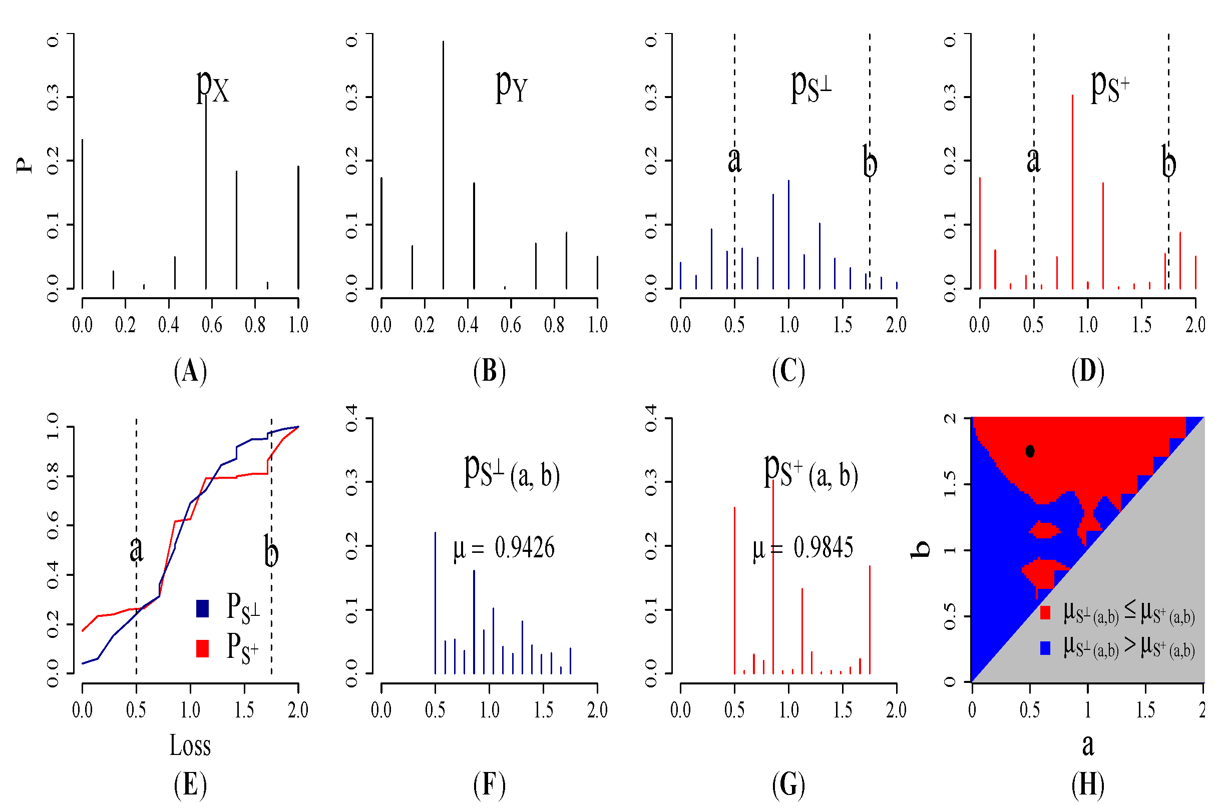
2.3. Ordering the Gross Loss Sums

We recall that, by construction, a positively dependent sum of ground-up risks satisfies convex ordering in (6). During gross loss aggregation, this sequencing can be impacted by financial terms. For comparing gross loss sums, it is convenient to use the stop-loss order ${\le }_{sl}$ related to the convex order by:

$$\left.\begin{array}{cc}\hfill & X{\le }_{sl}Y\hfill \\ \hfill & \mathrm{E}\left[X\right]=\mathrm{E}\left[Y\right]\hfill \end{array}\right\}\iff X{\le }_{cx}Y$$

(23)

There are two fundamental compositions (Theorems D1 and D2, Chapter 6 in Marshall et al. 1979) of supermodular functions that guarantee preservation of the stop-loss order. The first composition passes supermodular $\psi :{\mathbb{R}}^m\to \mathbb{R}$ as an argument to convex and non-decreasing $\varphi :\mathbb{R}\to \mathbb{R}$ resulting in the supermodular $g=\varphi \circ \psi$; see, e.g., Figure 2B,D. When applied to (6) we have:

$$\varphi (X_1^{\perp }+X_2^{\perp }+\dots +X_m^{\perp }){\le }_{sl}\varphi (X_1+X_2+\dots +X_m){\le }_{sl}\varphi (X_1^{+}+X_2^{+}+\dots +X_m^{+})$$

(24)

The second supermodular composition $g=\psi ({\varphi }_1,\dots ,{\varphi }_m)$ is comprised of the supermodular $\psi :{\mathbb{R}}^m\to \mathbb{R}$ and ${\varphi }_i:\mathbb{R}\to \mathbb{R}$, $i=1,\dots ,m$, which are all non-decreasing or all non-increasing; see, e.g., Figure 2C,F and Example 6.3.11 in Denuit et al. (2005). When applied to the individual summands constituting (6), we obtain:

$$\begin{array}{cc}\hfill {\varphi }_1{\left(X_1\right)}^{\perp }+{\varphi }_2{\left(X_2\right)}^{\perp }+\dots +{\varphi }_m{\left(X_m\right)}^{\perp }& {\le }_{sl}{\varphi }_1\left(X_1\right)+{\varphi }_2\left(X_2\right)+\dots +{\varphi }_m\left(X_m\right)\hfill \\ \hfill & {\le }_{sl}{\varphi }_1{\left(X_1\right)}^{+}+{\varphi }_2{\left(X_2\right)}^{+}\dots +{\varphi }_m{\left(X_m\right)}^{+}\hfill \end{array}$$

(25)

For the financial terms in Section 2.2, the precedence (25) always holds true. On the other hand, the precedence (24) holds true only for (18). For (19), the sign of inequality changes and loss precedence follows the concave order. For (20) and for the ith layer $L_X^{\left(i\right)}(t_{i-1},t_i)$ in (22), the problem is more complicated because $\varphi$ is neither convex nor concave. To proceed in such a case, we invoke the notion of the truncation transform in Hürlimann (1998), which replaces a random variable X with:

$$X(a,b)=X-{(a-X)}_{+}-{(X-b)}_{+}$$

(26)

on the finite interval $[a,b]$ for $-\infty <a,b<\infty$. For two random variables X and Y that satisfy $X{\le }_{sl}Y$, to establish if

$$X(a,b){\le }_{sl}Y(a,b)$$

(27)

holds, we use the Karlin–Novikoff–Stoyan–Taylor multiple-crossing conditions for $P_X$ and $P_Y$ (Karlin and Novikoff 1963; Stoyan and Daley 1983; Taylor 1983) and (Theorems 2.1 and A.1 in Hürlimann 1998) to demand that

$$\mathrm{E}\left[X\right(a,b\left)\right]\le \mathrm{E}\left[Y\right(a,b\left)\right]$$

(28)

and that either

$$P_X\left(b\right)>P_Y\left(b\right)$$

(29)

or b is the crossing point for the marginals

$$P_X\left(b\right)=P_Y\left(b\right)$$

(30)

such that the sign change of $P_Y\left(x\right)-P_X\left(x\right)$ in the neighborhood of b is from “-” to “+”. An example explaining the role of requirements (28) and (29) is shown in Figure 3.

Since (20) can be rewritten as:

$$min({(X-d)}_{+},l)=X(d,d+l)-d,$$

(31)

determining if (6) is preserved after application of a deductible and limit comes down to checking if

$$S^{\perp }(d,d+l){\le }_{sl}S(d,d+l){\le }_{sl}{S}^{+}(d,d+l)$$

(32)

is true using (29) or (30). Accordingly, for XOL layers we require

$$S^{\perp }(t_{i-1},t_i){\le }_{sl}S(t_{i-1},t_i){\le }_{sl}{S}^{+}(t_{i-1},t_i)$$

(33)

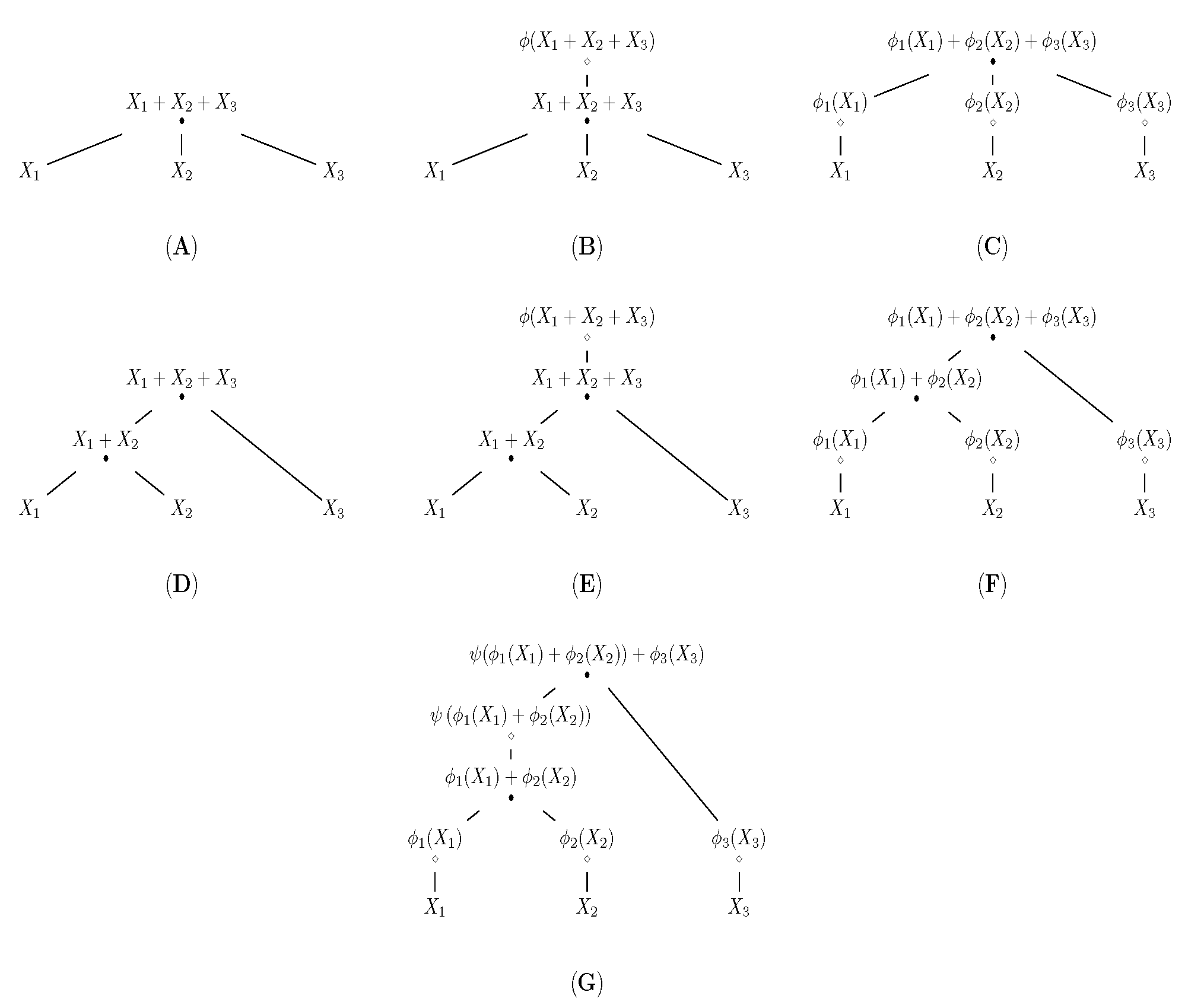
3. Partial Sums and Aggregation Trees

The weighted average in (10), referred to as the mixture method in Wang (1998), corresponds to the direct aggregation model in Wójcik et al. (2019). In situations where the partial sum $S_I={\sum }_{i\in I}{X}_i$ is of interest for any subset $I\subseteq \{1,\dots ,m\}$, loss aggregation can be performed by decomposing the positively dependent sum S using the bivariate hierarchical aggregation model in Wójcik et al. (2019). First, we select the two risks $X_i,X_j$ and define a bivariate dependency model as, e.g., the one in (9) for that pair. Then, we compute the partial sum $X_i+X_j$ and treat it as a new, integrated risk. The procedure can be reiterated with the remaining $m-1$ risks until a single total sum has been computed. The hierarchical models can be visualized as aggregation trees (see examples in Figure 2), which describe collection of relationships between pairs of risks and provide a bottom-up view of the total risk.

When constructing a bivariate aggregation tree, we first need to identify the tree topology, i.e., the order in which the risks are accumulated. Algorithms for computing the order of risk additions for ground-up loss are discussed in Wójcik et al. (2019). For gross loss, the tree topology is defined by the hierarchy of financial terms. The following is how a typical catastrophe insurance portfolio is organized. First, the location terms in (18), (19) or (20) are applied on individual risks. Then, locations tend to aggregate to the sub-limits expressed as (18), (19) or (20) and applied to a geographical subset of the total set of locations, such as, e.g., ZIP code. Thereafter, partial aggregates enter the XOL layers in (21). Next, the layer losses are accumulated to insurance policies using comonotonic addition in (22). Finally, policy losses are summed up to portfolio-level gross loss. We use sequential order of aggregation to sum up risks going into the same financial structure, e.g., an XOL layer and for final accumulation to the event loss total. An example for three risks is shown in Figure 2E. Based on the results in Wójcik et al. (2019), see Table 1 on p. 15, the sequential order is a good compromise, and offers good examples, between simplicity of implementation and accuracy of reproduction of tail statistics of partial aggregate risks as compared to large-sample Monte Carlo runs.

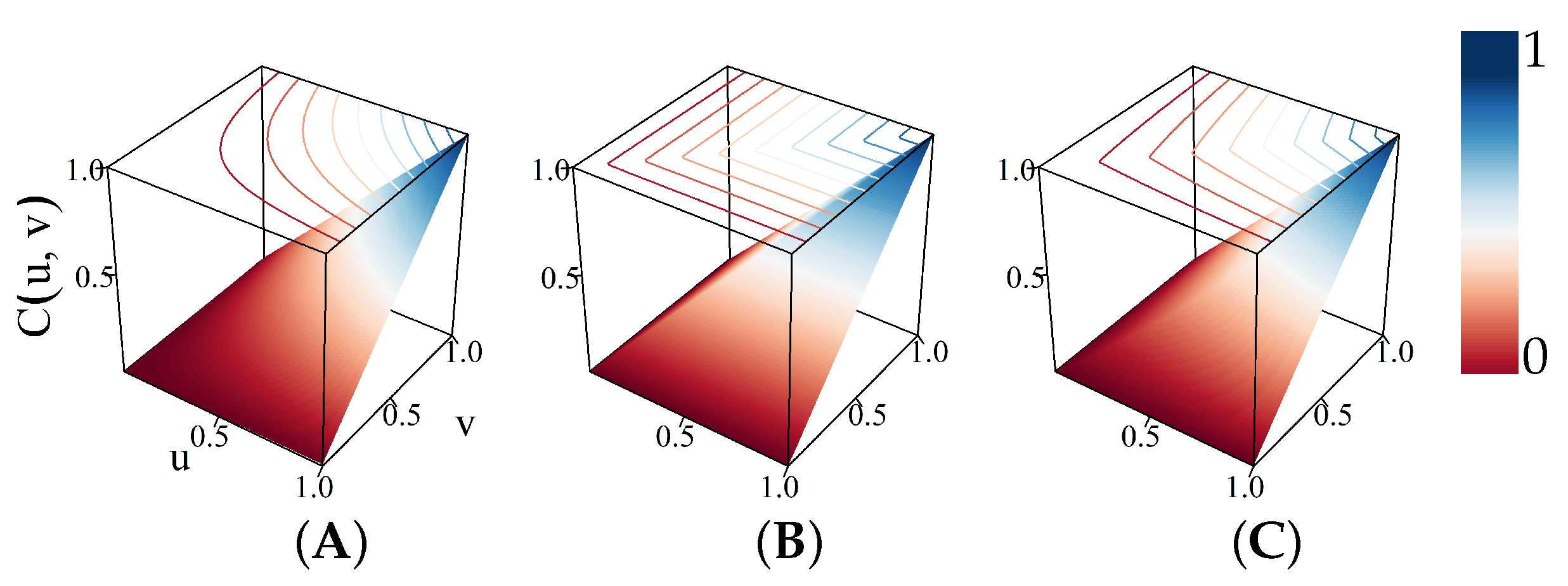
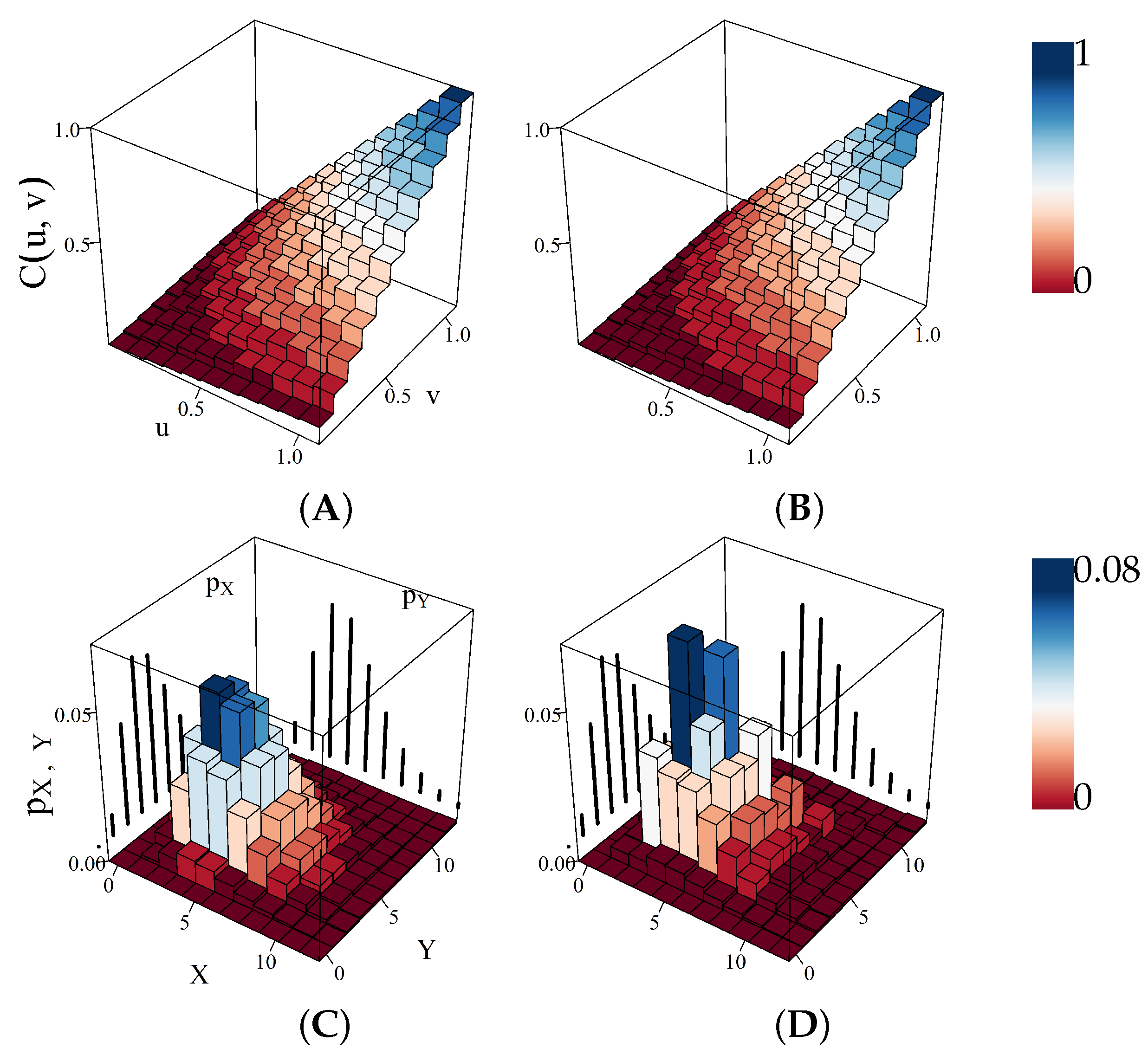
3.1. Copulas at Summation Nodes

The second step in constructing an aggregation tree is to provide a description of the bivariate joint distribution $P_{X,Y}$ for each pair of risks $X,Y$ with the marginals $P_X,P_Y$ entering a typical summation node in Figure 4A. In this study, we focus on the bivariate copula functions $C:{[0,1]}^2\to [0,1]$, which, by Sklar’s theorem (Sklar 1959), provide the following representation of the joint distribution:

$$P_{X,Y}(x,y)=C(P_X\left(x\right),P_Y\left(y\right))$$

(34)

It follows from the stochastic order in (2) that for any bivariate copula

$$C^{\perp }(u,v)\le C(u,v)\le C^{+}(u,v)$$

(35)

where $C^{\perp }(u,v)=uv$ is the independence copula and $C^{+}(u,v)=min\left(uv\right)$ is the comonotonicity copula for $u,v\in {[0;1]}^2$, respectively. A mixture of these two distributions

$$C_w(u,v)=(1-w)C^{\perp }(u,v)+w{C}^{+}(u,v)$$

(36)

is designated a Fréchet family in Denuit et al. (2002); an example is shown in Figure 5. Other bivariate copulas used in this paper are listed in

Table 1. Six common bivariate copula families.

Name	$\mathit{C}(\mathit{u},\mathit{v};\mathit{\theta })$	Parameter $\mathit{\theta }$
Fréchet	$(1-\theta )uv+\theta min(u,v)$	$\theta \in [0,1]$
Gaussian *	${\Phi }_{\Sigma }\left[{\Phi }^{-1}\left(u\right),{\Phi }^{-1}\left(v\right);\theta \right]$	$\theta \in [0,1]$
Student’s t **	${\int }_{-\infty }^x{\int }_{-\infty }^y{\left(2\pi \sqrt{1-{\theta }^2}\right)}^{-1}{\left[1+\frac{x^2-2\theta xy+y^2}{\nu (1-{\theta }^2)}\right]}^{-(\nu +2)/2}dxdy$, $x=P_{\nu }^{-1}\left(u\right)$, $y=P_{\nu }^{-1}\left(v\right)$	$\theta \in [-1,1]$
Gumbel	$exp\left\{-{\left({[-ln\left(u\right)]}^{\theta }+{[-ln\left(v\right)]}^{\theta }\right)}^{1/\theta }\right\}$	$\theta \in [1,+\infty )$
Joe	$1-{\left[{(1-u)}^{\theta }+{(1-v)}^{\theta }-{(1-u)}^{\theta }{(1-v)}^{\theta }\right]}^{1/\theta }$	$\theta \in [1,+\infty )$
Morgenstern	$uv[1+\theta (1-u\left)\right(1-v\left)\right]$	$\theta \in [0,1]$

* Φ⁻¹ is the inverse cdf of a standard normal, and Φ_Σ is the standard bivariate normal cdf with the covariance matrix Σ parameterized by θ. ** $P_{\nu }^{-1}$ is the inverse cdf of a standard Student’s t with v ∈ {1, 3, 10, 30} degrees of freedom. In this paper, v is chosen a priori and not subject to the optimization in Algorithm 1; The parameter θ is bounded by [−1,1] instead of [0,1] because negative θ in copula could still imply positive dependence in bivariate joint distribution estimated in Algorithm 1.

. They include a variety of distributions often used in insurance applications: two elliptical distributions (Gaussian and Student’s t), two Archimedean distributions (Gumbel and Joe) and a Morgenstern distribution obtained by adding a perturbation to the independence copula; see, e.g., Bouyé et al. (2000); Joe (1997) for a detailed discussion of probability density shapes and joint tail behavior, and Section 5 for discussion of the impact of these properties on gross loss estimates. We further discretize any continuous copula C in Table 1 using the methodology from Section 7.1 in Geenens (2020). We define the $(R\times O)$ discrete copula pmf as:

$$\begin{array}{cc}\hfill c(\frac{i+1}{R},\frac{j+1}{O})=& C\left(\frac{i+1}{R},\frac{j+1}{O}\right)-C\left(\frac{i+1}{R},\frac{j}{O}\right)\hfill \\ \hfill -& C\left(\frac{i}{R},\frac{j+1}{O}\right)+C\left(\frac{i}{R},\frac{j}{O}\right)\hfill \end{array}$$

(37)

where $(i,j)\in \left\{0,\dots ,R-1\right\}\times \left\{0,\dots ,O-1\right\}$. This discretization guarantees that the marginals of the copula pmf are uniform, i.e., ${\sum }_{j}c(\frac{i+1}{R},\frac{j+1}{O})=\frac{1}{R}$ and ${\sum }_{i}c(\frac{i+1}{R},\frac{j+1}{O})=\frac{1}{O}$; see Appendix B for details. The distribution $p_S$ of the sum $S=X+Y$ is then expressed as the discrete copula convolution:

$$p_{X+Y}\left(s\right)=\sum _{x}c\left(P_X\left(x\right),P_Y(s-x)\right)p_Y(s-x)$$

(38)

Note that if (34) can be approximated using (9), we obtain Fréchet decomposition of the copula C:

$$C(P_X\left(x\right),P_Y\left(y\right))\approx (1-w)C^{\perp }(P_X\left(x\right),P_Y\left(y\right))+w{C}^{+}(P_X\left(x\right),P_Y\left(y\right))$$

(39)

where the weight w is the comonotonicity coefficient in Koch and De Schepper (2006, 2011) defined as:

$$w=\frac{{\sum }_x{\sum }_y\left[C(P_X\left(x\right),P_Y\left(y\right))-P_X\left(x\right)P_Y\left(y\right)\right]}{{\sum }_x{\sum }_y\left[min(P_X\left(x\right),P_Y\left(y\right))-P_X\left(x\right)P_Y\left(y\right)\right]}$$

(40)

Algorithm 1 Estimate copula parameter and add two risks in ground-up pass

INPUT: Pmfs $p_X$, $p_Y$ with support sizes $N_x$, $N_y$, copula $C(u,v;\theta )$, (if available) partial derivative $C^{\prime }(u,v;\theta )=\partial C(u,v;\theta )/\partial \theta$, initial ${\theta }_0$ and bounds ${\theta }_{min}$, ${\theta }_{max}$, correlation $\rho (X,Y)$, maximum iteration $t_{max}$, numeric tolerance $ϵ$. OUTPUT: ${\theta }^{*}$, $p_S$. 1: Compute the means ${\mu }_X$, ${\mu }_Y$, standard deviations ${\sigma }_X$, ${\sigma }_Y$, and cdfs $P_X$, $P_Y$. 2: Goto Step 19 if $C^{\prime }(u,v;\theta )$ does not exist. 3: ${\theta }^{*}\leftarrow {\theta }_0$; $\gamma \leftarrow 0$. // $\gamma$ records boundary collisions. 4: for$t=1$ to $t_{max}$ do 5:      $P(x_i,y_j)\leftarrow C\left(P_X\left(x_i\right),P_Y\left(y_j\right);{\theta }^{*}\right)$, $1\le i\le N_x$, $1\le j\le N_y$. // Joint cdf. 6:      $p(x_i,y_j)\leftarrow P(x_i,y_j)-P(x_{i-1},y_j)-P(x_i,y_{j-1})+P(x_{i-1},y_{j-1})$. // Joint pmf. 7:      $P^{\prime }(x_i,y_j)\leftarrow C^{\prime }\left(P_X\left(x_i\right),P_Y\left(y_j\right);{\theta }^{*}\right)$. 8:     $p^{\prime }(x_i,y_j)\leftarrow P^{\prime }(x_i,y_j)-P^{\prime }(x_{i-1},y_j)-P^{\prime }(x_i,y_{j-1})+P^{\prime }(x_{i-1},y_{j-1})$. 9:      ${\rho }^{\star }(X,Y)\leftarrow \left[{\sum }_{i=1}^{N_x}{\sum }_{j=1}^{N_y}{x}_i{y}_{j}p(x_i,y_j)-{\mu }_X{\mu }_Y\right]/\left({\sigma }_X{\sigma }_Y\right)$. // Correlation given ${\theta }^{*}$. 10:     ${\rho }^{\prime }(X,Y)\leftarrow \left[{\sum }_{i=1}^{N_x}{\sum }_{j=1}^{N_y}{x}_i{y}_j{p}^{\prime }(x_i,y_j)-{\mu }_X{\mu }_Y\right]/\left({\sigma }_X{\sigma }_Y\right)$ 11:     ${\theta }^{*}\leftarrow min\left({\theta }_{max},max({\theta }_{min},{\theta }^{*}-({\rho }^{\star }(X,Y)-\rho (X,Y))/{\rho }^{\prime }(X,Y))\right)$ // Newton’s method update. 12:     if $|{\rho }^{\star }(X,Y)-\rho (X,Y)|\le ϵ$ then break // Found root. 13:     end if 14:     $\gamma \leftarrow \gamma +(\theta \le {\theta }_{min}\vee \theta \ge {\theta }_{max})$. // Increment $\gamma$ if the update collided with boundary. 15:     if $\gamma \ge 3$ then break // Newton’s method will not converge. 16:     end if 17: end for 18: if$\gamma \ge 3\vee t\ge t_{max}$then // Newton’s method failed. Try bisection. 19:      ${\theta }_{\mathrm{low}}\leftarrow {\theta }_{min}$; ${\theta }^{*}\leftarrow {\theta }_0$; ${\theta }_{\mathrm{high}}\leftarrow {\theta }_{max}$. 20:     for $t=1$ to $t_{max}$ do 21:         Compute ${\rho }^{\star }(X,Y)$ given ${\theta }^{*}$ following Steps 5, 6 and 9. 22:         if ${\rho }^{\star }(X,Y)-\rho (X,Y)<-ϵ$then${\theta }_{\mathrm{low}}\leftarrow {\theta }^{*}$. ${\rho }^{\star }(X,Y)-\rho (X,Y)>ϵ$${\theta }_{\mathrm{high}}\leftarrow {\theta }^{*}$. 23:         elsebreak 24:         end if 25:         ${\theta }^{*}\leftarrow ({\theta }_{\mathrm{low}}+{\theta }_{\mathrm{high}})/2$. 26:     end for 27:     ${\theta }^{*}\leftarrow (t<t_{max}){\theta }^{*}+(t\ge t_{max}){\theta }_{min}$. // If root not found, set ${\theta }^{*}$ to ${\theta }_{min}$. 28: end if 29: Execute Steps 5 and 6. 30: $p_S\leftarrow \mathbf{0}$; $p_S(x_i+y_j)\leftarrow p_S(x_i+y_j)+p(x_i,y_j)$, $1\le i\le N_x$, $1\le j\le N_y$. 31: return${\theta }^{*}$, $p_S$.

Figure 6 visualizes this idea. For the uniform $[0;1]$ marginals, (39) is equivalent to the statement $C\approx C_w$ and (40) equals the Spearman correlation ${\rho }_s(X,Y)$; (see Proposition 3 in Koch and De Schepper 2011). As shown in Dhaene et al. (2014), we can simplify (40) to:

$$w=\frac{\mathrm{Cov}[X,Y]}{\mathrm{Cov}[X^{+},Y^{+}]}$$

(41)

The pmf of the sum $X+Y$ is then given by (10), where its independent component is computed as:

$$p_{X^{\perp }+Y^{\perp }}\left(s\right)=\sum _x{p}_X\left(x\right)p_Y(s-x)$$

(42)

and its comonotonic component by differencing:

$$P_{X^{+}+Y^{+}}\left(s\right)=sup\left\{q\in [0;1]:P_X^{-1}\left(q\right)+P_Y^{-1}\left(q\right)<s\right\}$$

(43)

using, e.g., the algorithms in Wójcik et al. (2019). The key to application of (34) as a dependency model for the gross loss summation in Figure 4B is the copula invariance:

$$\begin{array}{ccc}\hfill C_{{\varphi }_X\left(X\right),{\varphi }_Y\left(Y\right)}(P_{{\varphi }_X\left(X\right)}\left(x^{{}^{\prime }}\right),P_{{\varphi }_Y\left(Y\right)}\left(y^{{}^{\prime }}\right))=& C_{X,Y}(P_X\left({\varphi }_X^{-1}\left(x^{{}^{\prime }}\right)\right),P_Y\left({\varphi }_Y^{-1}\left(y^{{}^{\prime }}\right)\right)\hfill & \\ \hfill =& C_{X,Y}(P_{{\varphi }_X\left(X\right)}\left(x^{{}^{\prime }}\right),P_{{\varphi }_Y\left(Y\right)}\left(y^{{}^{\prime }}\right))\hfill \end{array}$$

(44)

under any non-decreasing transformations ${\varphi }_X,{\varphi }_Y$ such as, e.g., those representing the financial terms in Section 2.2. As a consequence, the pmf $p_{{\varphi }_X\left(X\right)+{\varphi }_Y\left(Y\right)}$ is determined by plugging the marginals $p_{{\varphi }_X\left(X\right)},p_{{\varphi }_Y\left(Y\right)}$ into (38) or, if Fréchet decomposition is used, into (39), with the weight expressed as:

$$w=\frac{\mathrm{Cov}[{\varphi }_X\left(X\right),{\varphi }_Y\left(Y\right)]}{\mathrm{Cov}[{\varphi }_X\left(X^{+}\right),{\varphi }_Y\left(Y^{+}\right)]}$$

(45)

Finally, we remark that any copula family in Table 1 is positively ordered, which implies that

$$C(u,v;{\theta }_1)\le C(u,v;{\theta }_2)$$

(46)

for ${\theta }_1\le {\theta }_2$ and for all $u,v\in [0;1]$. From this inequality, we can easily see that for the weight in (40) written as a function of $\theta$, we have:

$$w\left({\theta }_1\right)\le w\left({\theta }_2\right)$$

(47)

3.2. Covariance Scaling

When the available statistical descriptors are limited to only the marginals $p_X,p_Y$ and the covariance $\mathrm{Cov}[X,Y]$, and computing speed is of particular importance (see, e.g., Wang 1998; Wójcik et al. 2019), it is advantageous to use the Fréchet copula in (36) as opposed to using the Fréchet decomposition in (39) of any other copula in Table 1; see Section 4 for details. For the ground-up summation $X+Y$ in Figure 4A, the weight is computed using (41). For the gross loss summation ${\varphi }_X\left(X\right)+{\varphi }_Y\left(Y\right)$ in Figure 4B, the weight is computed using (45). In this case we first obtain the transformed marginals $p_{{\varphi }_X},p_{{\varphi }_Y}$ using (15). Next, we express the (unknown) covariance $\mathrm{Cov}[{\varphi }_X\left(X\right),{\varphi }_Y\left(Y\right)]$ in the numerator of (45) by precising the condition (1) in Section 2, i.e.,

$$\mathrm{Cov}[{\varphi }_X\left(X\right),{\varphi }_Y\left(Y\right)]={\alpha }_{X,Y}\mathrm{Cov}[X,Y]$$

(48)

Finally, we use (implicit) affine transformations of the ground-up risks:

$$\begin{array}{c}\hfill \tilde{X}=\frac{{\sigma }_{{\varphi }_X\left(X\right)}}{{\sigma }_X}X+{\beta }_X\end{array}$$

(49)

$$\begin{array}{c}\hfill \tilde{Y}=\frac{{\sigma }_{{\varphi }_Y\left(Y\right)}}{{\sigma }_Y}Y+{\beta }_Y\end{array}$$

(50)

where ${\sigma }_X,{\sigma }_Y$ and ${\sigma }_{{\varphi }_X\left(X\right)},{\sigma }_{{\varphi }_Y\left(Y\right)}$ are ground-up and gross loss standard deviations for individual risks, respectively, to write the gross loss weight as:

$$w=\frac{{\alpha }_{X,Y}\mathrm{Cov}[X,Y]}{\mathrm{Cov}[{\varphi }_X\left(X^{+}\right),{\varphi }_Y\left(Y^{+}\right)]}=\frac{\mathrm{Cov}[\tilde{X},\tilde{Y}]}{\mathrm{Cov}[{\varphi }_X\left(X^{+}\right),{\varphi }_Y\left(Y^{+}\right)]}$$

(51)

where

$${\alpha }_{X,Y}=\frac{{\sigma }_{{\varphi }_X\left(X\right)}{\sigma }_{{\varphi }_Y\left(Y\right)}}{{\sigma }_X{\sigma }_Y}$$

(52)

Note that such ansatz does not alter the integration scheme in Figure 4B. It only approximates the gross loss weight computation when the dependence structure is given by (36). The advantage is the substantial gain in computational speed of loss integration as compared to using the copula convolution in (38); for details see Section 4.

3.3. A Comment on Back Allocation

We point out that (49) and (50) are inspired by the procedure of partitioning the gross loss sum ${\varphi }_X\left(X\right)+{\varphi }_Y\left(Y\right)$ back to individual risk level $\tilde{X}$ and $\tilde{Y}$. Defining the offsets in (49) and (50) as:

$$\begin{array}{ccc}\hfill {\beta }_X& =& {\mu }_{{\varphi }_X\left(X\right)}-\frac{{\sigma }_{{\varphi }_X\left(X\right)}}{{\sigma }_X}{\mu }_X\hfill \end{array}$$

(53)

$$\begin{array}{ccc}\hfill {\beta }_Y& =& {\mu }_{{\varphi }_Y\left(Y\right)}-\frac{{\sigma }_{{\varphi }_Y\left(Y\right)}}{{\sigma }_Y}{\mu }_Y\hfill \end{array}$$

(54)

where ${\mu }_X,{\mu }_Y$ and ${\mu }_{{\varphi }_X\left(X\right)},{\mu }_{{\varphi }_Y\left(Y\right)}$ are ground-up and gross loss means for individual risks, respectively, guarantees that

$$\begin{array}{ccc}\hfill \mathrm{E}[{\varphi }_X\left(X\right)+{\varphi }_Y\left(Y\right)]& =& \mathrm{E}[\tilde{X}+\tilde{Y}]\hfill \end{array}$$

(55)

$$\begin{array}{ccc}\hfill \mathrm{Var}[{\varphi }_X\left(X\right)+{\varphi }_Y\left(Y\right)]& =& \mathrm{Var}[\tilde{X}+\tilde{Y}]\hfill \end{array}$$

(56)

In catastrophe insurance, this procedure is referred to as back allocation; see, e.g., Mitchell-Wallace et al. (2017). By replacing the integration node in Figure 4B with its second-order proxy in Figure 4C, the back-allocated losses are sometimes used to evaluate the impact of financial terms on specific geographical/administrative groups of risks. For example, two groups of risks that belong to different insurance policies and are subject to different policy limits may contain subsets of risks that belong to one county. Therefore, back allocation is needed if county-level gross loss is of interest. We stress that preservation of the second-order moments in (55) and (56) makes our new back allocation method an extension of the more traditional approach in Mitchell-Wallace et al. (2017), which satisfies only (55) by prorating higher-level financial structure mean loss in proportion to the lower-level mean loss(es). In this study, we do not use back allocation per se, so we leave further investigation of the new method for future research.

4. Computational Aspects

Our bivariate copula approach requires two separate passes of risk summation over an aggregation tree: ground-up pass and gross loss pass. The former is performed to identify the parameters of copulas at the summation nodes in Figure 4A such that they reproduce imposed ground-up covariance. The gross loss pass is performed to obtain an estimate of the total insured loss pmf using the summation nodes in Figure 4B. with copulas parameterized during the ground-up pass. The order of summations (tree topology) is fixed for both passes and, as mentioned in Section 3, dictated by the structure of financial terms and sequential order of aggregation; compare, e.g., the sequential gross loss aggregation tree in Figure 2G, which determines the order of ground-up summation in Figure 2B. In the course of the ground-up pass, at each summation node the marginals $P_X$ and $P_Y$, the parametric copula $C(u,v;\theta )$ (see Table 1) and the covariance $\mathrm{Cov}[X,Y]$ are given. Our objective is to find:

$$\begin{array}{c}\hfill {\theta }^{\star }=\underset{\theta }{min}\left|\mathrm{Cov}[X,Y]-\sum _x\sum _y\left[C(P_X\left(x\right),P_Y\left(y\right);\theta )-P_X\left(x\right)P_Y\left(y\right)\right]\right|\end{array}$$

(57)

This corresponds to matching the prescribed Person’s correlation $\rho (X,Y)$ with its copula-based counterpart ${\rho }^{\star }(X,Y)$ obtained by integrating $C(P_X\left(x\right),P_Y\left(y\right);{\theta }^{\star })$. It trivially follows that the target variance

$$\mathrm{Var}[X+Y]=\sum _x\sum _y\left[C(P_X\left(x\right),P_Y\left(y\right);{\theta }^{\star })\right]$$

(58)

is reproduced at each node of the ground-up aggregation tree. Algorithm 1 offers a numerical solution to (57). Newton’s method (see, e.g., Kelley 2003) is invoked first, and if it fails, the bisection method in Sikorski (1982) is called. Failure occurs when Newton’s update, which initially falls outside $\theta$’s domain, is capped at the boundary. As a result, the algorithm triggers an infinite loop of bouncing back and forth between the boundary and the points within the domain. Both Newton’s and bisection optimizers require $O\left(N_x{N}_y\right)$ time and space in each iteration. Newton’s method takes extra time to evaluate the derivative in Step 7, but it usually converges much faster than the bisection method (Ehiwario and Aghamie 2014).

For Gaussian copula, the optimization procedure in Xiao and Zhou (2019) is applied to computing ${\rho }^{\star }(X,Y)$ in Algorithm 1, Step 9. The idea is to approximate a bivariate Gaussian pdf with Hermite polynomials and to subsequently reduce the correlation function of $\theta$ to polynomial series. Acceleration due to this technique is substantial because of Newton’s method’s suitability for solving polynomials. In our implementation, the Taylor expansion (Equation 39 in Xiao and Zhou 2019) stops when the rightmost term becomes less than 0.00001. For Student’s t copula, $\theta$ is bounded by $[-1,1]$ instead of $[0,1]$ while being optimized in Algorithm 1. This is because negative $\theta$ in the copula could still imply positive dependence in bivariate joint distribution. If spurious negative correlation between the marginal risks is detected during the gross loss pass, we proceed assuming independence and using discrete convolution. Numeric threshold $ϵ$ and maximum iteration $t_{max}$ in Algorithm 1 are set to 0.0001 and 1000, respectively. These values provide a reasonable balance between numeric precision and computing speed.

Next, the gross loss pass is performed with Algorithm 2 using copulas optimized in the ground-up pass. The algorithm implements the summation node in Figure 4B. The dominant computational overhead comes from Step 2, which has both asymptotic space consumption and asymptotic time complexity of $O\left(N_x{N}_y\right)$. The latter is due to processing primitive arithmetic such as exponentiation and logarithm, which constitute most copulas listed in Table 1. Speed comparison with other fundamental operations, e.g., addition and multiplication, is shown in

Table 2. Actual (relative) execution times in microseconds of calling primitive functions for 10,000,000 times on double-precision floating-point numbers generated at random. Platform: Intel i9-9980HK CPU, 32 GB RAM, Windows 10. Compiler: Mingw-w64 g++ 8.3 -std=gnu++17 -Ofast -mfpmath=sse -msse2 -mstackrealign.

$\mathit{a}+\mathit{b}$	$\mathbf{a}\mathbf{b}$	$exp\left(\mathit{a}\right)$	$ln\mathit{a}$	${\mathit{a}}^{\mathit{b}}$	$arctan\left(\mathit{a}\right)$
5593 (1)	6130 (1.1)	315,567 (56.4)	209,969 (37.5)	670,001 (119.8)	130,785 (23.4)

. In Step 7, the copula decomposition in (39) is performed. This variant, however, is slower than the original copula approach. It requires both computing the bivariate joint in (39) and the mixture distribution of the sum in (10) with the weight in (45). Computation of the mixture has asymptotic space complexity of $O(N_x+N_y)$ due to auxiliary memory allocations entailed in regridding and estimating the comonotonic sum (Algorithms 3, 6 in Wójcik et al. 2019) and asymptotic time complexity of $O\left(N_x{N}_y\right)$ dominated by the convolution algorithm (Section 2.4.1 Wójcik et al. 2019). We point out that the covariance scaling approach in Section 3.2 does not require the ground-up pass. The weight in (45) depends only on the scaled covariance and the transformed marginals, both computed adaptively during the gross loss pass.

Algorithm 2 Add two risks in gross loss pass

INPUT: Pmfs $p_{{\varphi }_X\left(X\right)}$, $p_{{\varphi }_Y\left(Y\right)}$ with support sizes $N_x$, $N_y$, parameterized copula model $C(u,v;{\theta }^{\star })$, decomposition flag. OUTPUT: Pmf $p_{\varphi \left(S\right)}$ of the gross loss sum $\varphi \left(S\right)={\varphi }_X\left(X\right)+{\varphi }_Y\left(Y\right)$. 1: Compute cdfs $P_{{\varphi }_X\left(X\right)}$ and $P_{{\varphi }_Y\left(Y\right)}$. // Time $O(N_x+N_y)$. Space $O\left(1\right)$. 2: Compute the joint cdf $P_{{\varphi }_X\left(X\right),{\varphi }_Y\left(Y\right)}\leftarrow C\left(P_{{\varphi }_X\left(X\right)}\left(x\right),P_{{\varphi }_Y\left(Y\right)}\left(y\right);{\theta }^{\star }\right)$. // Time $O\left(N_x{N}_y\right)$. Space $O\left(N_x{N}_y\right)$. 3: Compute pmf $p_{{\varphi }_X\left(X\right),{\varphi }_Y\left(Y\right)}$ by differencing $P_{{\varphi }_X\left(X\right),{\varphi }_Y\left(Y\right)}$ in place. // Time $O\left(N_x{N}_y\right)$. Space $O\left(1\right)$. 4: if decomposition flag is unset then 5:     Initialize $p_{\varphi \left(S\right)}\leftarrow \mathbf{0}$. 6:     Let $p_{\varphi \left(S\right)}(x+y)\leftarrow p_{\varphi \left(S\right)}(x+y)+p_{{\varphi }_X\left(x\right),{\varphi }_Y\left(y\right)}(x,y)$. // Time $O\left(N_x{N}_y\right)$. Space $O\left(1\right)$. 7: else// Invoke the mixture method. 8:     Compute w using (40). // Time $O\left(N_x{N}_y\right)$. Space $O\left(1\right)$. 9:     Make mixture $p_{\varphi \left(S\right)}\leftarrow (1-w)p_{\varphi {\left(S\right)}^{\perp }}+w{p}_{\varphi {\left(S\right)}^{+}}$. // Time $O\left(N_x{N}_y\right)$. Space $O(N_x+N_y)$. 10: end if 11: return$p_{\varphi \left(S\right)}$.

All algorithms were coded in C++. Bivariate Gaussian cdf implementation is based on the C code in the library by Donnelly (1973). Bivariate Student’s t cdf implementation converts the Fortran code in R package mvtnorm (see Genz et al. 2021) into C++. Figure 7 shows the time cost of adding two random variables using copulas in Table 1. The Fréchet copula with covariance scaling facilitates the fastest processing due to its uncomplicated form and adaptive parameter estimation in Algorithm 3. Slightly slower Morgenstern copula convolution takes advantage of the straightforward algebraic expression for bivariate cdf and constant $\partial C(u,v;\theta )/\partial \theta$; see Appendix A.3. Similarly, Student’s t algorithm with $\nu =1$ (Cauchy) gains efficiency from the uncomplicated derivative in Appendix A.4 and relatively fast arctan operation; see Table 2. When $\nu >1$, the bivariate Student’s t cdf has a sign function of $\theta$ that is not differentiable (Equations (10) and (11) in Dunnett and Sobel 1954). In this case, ${\theta }^{\star }$ is estimated by the bisection method in Algorithm 1. Because the cdf is evaluated in a recursion dependent on $\nu$, the computing time grows with increasing degrees of freedom. When Gaussian copula is used, evaluations of bivariate and inverse univariate Gaussian cdfs are needed. Both entail integrals of computationally expensive exponential functions, which makes risk integration slower than that based on Cauchy copula. Equations for Joe and Gumbel copulas and their partial derivatives contain compositions of power functions (see Appendix A.1 and Appendix A.2), which is the main reason for their longest processing times.

Algorithm 3 Add two risks in gross loss pass using Fréchet copula with covariance scaling

INPUT: Pmfs $p_X$ and $p_Y$, financial terms ${\varphi }_X$ and ${\varphi }_Y$, covariance $\mathrm{Cov}[X,Y]$. OUTPUT: Pmf of the sum $p_{\varphi \left(S\right)}$. 1: Compute standard deviations ${\sigma }_X$ and ${\sigma }_Y$. 2: Compute gross loss pmfs $p_{\varphi \left(X\right)}$, $p_{\varphi \left(Y\right)}$ and their standard deviations ${\sigma }_{{\varphi }_X\left(X\right)}$ and ${\sigma }_{{\varphi }_Y\left(Y\right)}$. 3: Compute the covariance scaling factor: ${\alpha }_{X,Y}\leftarrow {\sigma }_{{\varphi }_X\left(X\right)}{\sigma }_{{\varphi }_Y\left(Y\right)}/\left({\sigma }_X{\sigma }_Y\right)$. 4: Compute the comonotonic sum pmf $p_{\varphi {\left(S\right)}^{+}}$, and derive the comonotonic covariance $\mathrm{Cov}[{\varphi }_X\left(X^{+}\right),{\varphi }_Y\left(Y^{+}\right)]$. 5: Compute the gross loss weight w in (51). 6: Make mixture $p_{\varphi \left(S\right)}\leftarrow (1-w)p_{\varphi {\left(S\right)}^{\perp }}+w{p}_{\varphi {\left(S\right)}^{+}}$. 7: return$p_{\varphi \left(S\right)}$.

5. Results

To test the proposed algorithms for the copulas in Table 1, we computed gross loss for two major hurricane events and one major earthquake event in the United States. These natural catastrophes inflicted damage to 31,896, 9056 and 1209 locations, respectively, from three undisclosed commercial insurance portfolios. Some characteristics of these portfolios are shown in

Table 3. Characteristics of three representative catastrophe insurance portfolios.

Statistic	Portfolio 1 (Large)	Portfolio 2 (Medium)	Portfolio 3 (Small)
Event peril	Hurricane	Hurricane	Earthquake
# of risks	31,896	9056	1209
# of sub-limits	3364	412	19
# of layers	1778	398	14
# of policies	1676	398	14
Total replacement value ()MM USD)	671,191	25,811	14,350
Total ground-up loss	410	1198	427
Total ground-up damage ratio	0.06%	4.64%	0.41%

. Following the convention used in catastrophe insurance, we express risk as the damage ratio, i.e., loss over the replacement value. For each event, the damage ratio $X_k|I_k$ based on knowledge of the peril intensity $I_k$ at kth affected location is given by the catastrophe model prediction ${\zeta }_k|I_k$ and described by zero-inflated, limited transformed beta distribution (see Klugman et al. 2012; Ospina and Ferrari 2010). We assume that the mean of each distribution is determined by the expectation of model prediction and that covariance between risks characterizes model error, so

$$\begin{array}{cc}\hfill X_k|I_k& ={\zeta }_k|I_k+{\eta }_k\hfill \\ \hfill {\xi }_k|I_k& \sim \mathrm{Zero}-\mathrm{inflated},\mathrm{limited}TRB(r,s,\alpha ,\beta )\hfill \\ \hfill E\left[X_k\right|I_k]& =E\left[{\zeta }_k|I_k\right]=h\left(I_k\right)\hfill \\ \hfill \mathrm{Cov}\left[X_i|I_i,X_j|I_j\right]& ={\Sigma }_{i,j}=E\left[\left(X_i\right|I_i-h\left(I_i\right))\left(X_j\right|I_j-h\left(I_j\right))\right]\hfill \end{array}$$

(59)

where the zero-mean noise term $\eta$ represents the epistemic uncertainty in the catastrophe model development (see, e.g., Grossi 2004), and h is the damage function, which converts peril intensity to damage ratio. For hurricanes the intensity is expressed as wind speed and is computed using the U.S. hurricane model in AIR-Worldwide (2015). For earthquakes the intensity is measured as spectral acceleration of ground motion and is obtained from the U.S. earthquake model in AIR-Worldwide (2017). Loss distributions were discretized on a 64-point grid; some examples are shown in Figure 8. Spatial dependency was captured by the nested block diagonal correlation matrix $\mathbf{R}$ corresponding to the covariance matrix $\Sigma$ (see Figure 2B in Wójcik et al. 2019). This structure was because of imposing exchangeable correlation in spatial grid blocks at two scales using the random effects model in Einarsson et al. (2016). For hurricanes, the widths of spatial bins were 1 km and 20 km. The values assigned to off-diagonal entries were 0.07 if two risks were within the same 1 km block, and 0.02 if two risks resided in the same 20 km block but different 1 km blocks. Correlation was set to zero if any two risks belonged to different 20 km blocks. For earthquakes, the widths of the spatial bins were 1 km and 25 km, respectively, with the corresponding correlation coefficients 0.26 and 0.09. Any two risks from different 25 km blocks were considered uncorrelated.

The insurance hierarchy which determined the order of gross loss aggregation in each portfolio was: sub-limits, XOL layers and policies; see Section 3 for details and Table 3 for the number of components in each tier of financial terms. A hierarchical aggregation tree with sequential topology was chosen to perform gross loss accumulation; see, e.g., Figure 2. In all runs, at every summation node the support size of aggregate loss pmf was limited to 256 points, and losses with probabilities ≤${10}^{-10}$ were set to zero. This “tail truncation” was intended to maintain fine discretization at the bulk of the pmf, particularly during the ground-up pass. To speed up computations based on Fréchet copula with covariance scaling and those based on Frechèt decomposition, we used numerical convolution with linear regridding; see Algorithm A1 and Algorithm 3 in Wójcik et al. (2019). We also considered a multivariate extension of the Fréchet copula in (36) with a multivariate extension of the covariance scaling factor in (52). The multivariate Fréchet model uses the direct tree (see Figure 2A–C) to aggregate risks going into the same financial structure, e.g., a sub-limit. In other words, the summation nodes on an aggregation tree are followed by the transformation nodes (financial terms) in Figure 2, with the exception of when the risks are summed up to an event total, without breaking the summation into smaller bivariate chunks.

Total gross loss pmfs for Portfolios 1, 2 and 3 are presented in Figure 9, Figure 10 and Figure 11, respectively.

Table 4. Means, standard deviations and tail statistics (relative to multivariate Fréchet) of the aggregate gross loss pmfs.

	Portfolio 1 (Large)					Portfolio 2 (Medium)					Portfolio 3 (Small)
[MM $]	$\mu$	$\sigma$	TVaR${}_{\mathbf{1}\%}$	TVaR${}_{\mathbf{5}\%}$	TVaR${}_{\mathbf{10}\%}$	$\mu$	$\sigma$	TVaR${}_{\mathbf{1}\%}$	TVaR${}_{\mathbf{5}\%}$	TVaR${}_{\mathbf{10}\%}$	$\mu$	$\sigma$	TVaR${}_{\mathbf{1}\%}$	TVaR${}_{\mathbf{5}\%}$	TVaR${}_{\mathbf{10}\%}$
Multivariate Fréchet	293.2 (1.00)	276.5 (1.00)	1167.6 (1.00)	730.4 (1.00)	647.5 (1.00)	36.1 (1.00)	4.8 (1.00)	53.6 (1.00)	48.5 (1.00)	45.8 (1.00)	16.0 (1.00)	6.3 (1.00)	37.5 (1.00)	32.7 (1.00)	29.9 (1.00)
Fréchet	291.0 (0.99)	271.3 (0.98)	2000.7 (1.71)	1035.3 (1.42)	795.4 (1.23)	36.1 (1.00)	5.4 (1.12)	53.7 (1.00)	49.2 (1.01)	46.7 (1.02)	15.9 (1.00)	6.3 (1.00)	37.5 (1.00)	32.6 (1.00)	29.8 (1.00)
Gaussian	290.1 (0.99)	285.6 (1.03)	1626.9 (1.39)	1129.6 (1.55)	931.2 (1.44)	36.2 (1.00)	6.0 (1.25)	56.3 (1.05)	51.0 (1.05)	48.2 (1.05)	15.9 (1.00)	6.3 (1.00)	37.4 (1.00)	32.6 (1.00)	29.8 (1.00)
Gaussian decomp	290.6 (0.99)	279.9 (1.01)	2091.4 (1.79)	1085.4 (1.49)	823.6 (1.27)	36.2 (1.00)	6.0 (1.25)	57.4 (1.07)	51.2 (1.06)	48.2 (1.05)	15.9 (1.00)	6.3 (1.00)	37.6 (1.00)	32.6 (1.00)	29.8 (1.00)
Joe	291.2 (0.99)	183.6 (0.66)	1141.2 (0.98)	765.9 (1.05)	651.5 (1.01)	36.2 (1.00)	5.4 (1.13)	54.3 (1.01)	49.5 (1.02)	46.9 (1.02)	15.9 (1.00)	6.3 (1.00)	37.6 (1.00)	32.6 (1.00)	29.8 (1.00)
Joe decomp	291.4 (0.99)	183.5 (0.66)	1155.2 (0.99)	769.5 (1.05)	652.7 (1.01)	36.3 (1.00)	5.4 (1.13)	54.1 (1.01)	49.4 (1.02)	47.0 (1.03)	15.9 (1.00)	6.3 (1.00)	37.6 (1.00)	32.6 (1.00)	29.8 (1.00)
Gumbel	291.3 (0.99)	184.5 (0.67)	1138.9 (0.98)	767.9 (1.05)	654.1 (1.01)	36.3 (1.01)	5.5 (1.15)	55.1 (1.03)	50.0 (1.03)	47.4 (1.03)	15.9 (1.00)	6.3 (1.00)	37.6 (1.00)	32.6 (1.00)	29.8 (1.00)
Gumbel decomp	291.4 (0.99)	185.0 (0.67)	1175.8 (1.01)	773.9 (1.06)	654.8 (1.01)	36.1 (1.00)	5.5 (1.15)	54.1 (1.01)	49.5 (1.02)	47.0 (1.03)	15.9 (1.00)	6.3 (1.00)	37.6 (1.00)	32.6 (1.00)	29.8 (1.00)
Morgenstern	293.2 (1.00)	255.9 (0.93)	1101.3 (0.94)	908.7 (1.24)	812.4 (1.25)	36.2 (1.00)	6.0 (1.25)	55.4 (1.03)	50.7 (1.04)	48.1 (1.05)	15.9 (1.00)	6.3 (1.00)	37.4 (1.00)	32.6 (1.00)	29.8 (1.00)
Morgenstern decomp	293.2 (1.00)	238.9 (0.86)	1718.7 (1.47)	971.8 (1.33)	765.7 (1.18)	36.2 (1.00)	6.0 (1.25)	57.1 (1.06)	51.1 (1.05)	48.3 (1.05)	15.9 (1.00)	6.3 (1.00)	37.6 (1.00)	32.7 (1.00)	29.8 (1.00)
Student’s t, $\nu =1$	290.7 (0.99)	150.3 (0.54)	794.7 (0.68)	656.9 (0.90)	582.3 (0.90)	36.8 (1.02)	4.4 (0.93)	54.2 (1.01)	49.2 (1.01)	46.4 (1.01)	16.0 (1.00)	5.8 (0.92)	36.7 (0.98)	32.0 (0.98)	29.0 (0.97)
Student’s t decomp, $\nu =1$	290.7 (0.99)	154.1 (0.56)	788.2 (0.68)	656.9 (0.90)	585.1 (0.90)	36.3 (1.01)	5.1 (1.06)	53.4 (1.00)	48.9 (1.01)	46.6 (1.02)	16.0 (1.00)	5.8 (0.92)	36.7 (0.98)	32.0 (0.98)	29.0 (0.97)
Student’s t, $\nu =3$	290.9 (0.99)	151.1 (0.55)	916.9 (0.79)	677.7 (0.93)	592.9 (0.92)	36.5 (1.01)	4.3 (0.90)	55.6 (1.04)	49.4 (1.02)	46.1 (1.01)	16.0 (1.00)	6.0 (0.95)	37.1 (0.99)	32.3 (0.99)	29.4 (0.98)
Student’s t decomp, $\nu =3$	291.0 (0.99)	154.4 (0.56)	791.3 (0.68)	658.1 (0.90)	586.2 (0.91)	36.3 (1.00)	5.2 (1.08)	53.4 (1.00)	49.0 (1.01)	46.7 (1.02)	16.0 (1.00)	6.0 (0.96)	37.2 (0.99)	32.3 (0.99)	29.4 (0.98)
Student’s t, $\nu =10$	290.9 (0.99)	177.8 (0.64)	1194.1 (1.02)	794.4 (1.09)	663.0 (1.02)	36.7 (1.02)	5.2 (1.09)	60.0 (1.12)	51.8 (1.07)	48.2 (1.05)	15.9 (1.00)	6.2 (0.99)	37.5 (1.00)	32.6 (1.00)	29.7 (0.99)
Student’s t decomp, $\nu =10$	291.1 (0.99)	181.6 (0.66)	1124.2 (0.96)	761.4 (1.04)	649.1 (1.00)	36.3 (1.00)	5.3 (1.11)	53.8 (1.00)	49.2 (1.01)	46.9 (1.02)	15.9 (1.00)	6.3 (1.00)	37.5 (1.00)	32.6 (1.00)	29.7 (0.99)
Student’s t, $\nu =30$	290.9 (0.99)	256.2 (0.93)	1596.6 (1.37)	1056.0 (1.45)	854.9 (1.32)	36.1 (1.00)	5.8 (1.21)	57.7 (1.08)	51.3 (1.06)	48.2 (1.05)	15.8 (0.99)	6.4 (1.01)	37.9 (1.01)	32.7 (1.00)	29.7 (1.00)
Student’s t decomp, $\nu =30$	291.2 (0.99)	257.1 (0.93)	1884.1 (1.61)	1007.5 (1.38)	782.8 (1.21)	36.2 (1.00)	5.9 (1.22)	56.6 (1.06)	50.8 (1.05)	48.0 (1.05)	15.8 (0.99)	6.4 (1.01)	37.6 (1.00)	32.7 (1.00)	29.7 (1.00)

shows three statistics characterizing these distributions: mean ($\mu$), standard deviation ($\sigma$) and the expectation of loss conditional on the loss being greater than the 1st, 5th and 10th percentile, correspondingly ($1,5,10$%-TVaR; see, e.g., Artzner et al. 1999). In Portfolios 1, 2 and 3, over half of the total ground-up loss comes from the top 2.4%, 0.52% and 0.41% properties, respectively, with the largest replacement values. Policies written to expensive commercial properties typically have a share term on the XOL layer in (21). This linear term specifies that only a small ratio, e.g., 8%, of the XOL layer is covered. As a result, the loss reduction from ground-up to gross occurs by scaling the support of the gross loss distribution after application of the XOL layer. Accordingly, for each portfolio in Table 4, all copulas produce gross loss pmfs with similar expected values. On the other hand, variance of the total loss is impacted by the covariances between pairs of risks; hence, the heterogeneity in $\sigma$s is relatively high among different copulas. We observe that the variability declines, however, from Portfolios 1 to 3 as fewer buildings dominate the total replacement.

The ground-up total damage ratio of Portfolio 1 is only 0.06% (Table 3), and most marginal, location-level loss distributions are strongly right-skewed. When imposing a prescribed ground-up correlation between the long-tailed marginals, the correlation in the Gaussian copula usually takes higher values than the default correlation in joint distribution. Reason being, the Gaussian copula (family B1 in Joe 1997) is symmetric and concentrates on dependence in the bulk more than in the right tail of the bivariate distribution. Once the marginals become less skewed after financial terms have been applied, correlations between the gross losses are frequently inflated compared to the corresponding correlations between the ground-up losses. As a result, the Gaussian copula induces the highest variance of the total gross loss. For the Fréchet copula, this effect is attenuated by covariance scaling, which preserves the ground-up correlations. In the case of the Morgenstern copula (family B10 in Joe 1997), the positive correlation range is limited, i.e., for $\theta \in (0;1]$, the corresponding Spearman’s correlation is ${\rho }_s\in (0;1/3]$. Owing to this restriction, the gross loss variance is slightly lower than the variance for the Fréchet copula. In contrast, Joe and Gumbel copulas (families B5 and B6 in Joe 1997) are both designed to model the right tail dependence. They need only a small value of the dependence parameter $\theta$ (Table 1) to reproduce the imposed ground-up correlation between the marginals with heavy right tails. During the gross loss pass, probability mass of partial loss aggregates is shifted from tail to bulk of their pmfs, and as a result, correlation between the partial summands becomes weaker. This leads to the low variance of the total gross loss as compared to other copulas; see Figure 9.

In Portfolio 2, the marginals are significantly less skewed as compared to Portfolio 1. This is manifested by high value of the total ground-up damage ratio; see Table 3. For the Morgenstern copula, we can often find ${\theta }^{\star }<1$ to impose the prescribed correlation. Accordingly, the variance of the total gross loss matches that estimated using Gaussian copula and that estimated using the Fréchet decomposition of the Gaussian copula. We remark that in Figure 9, Figure 10 and Figure 11 the gross loss pmfs produced by the Fréchet decomposition have close $\sigma$s to their copula counterparts. To make this comparison more precise, for each copula and its Fréchet decomposition, we computed the percentage errors for $\mu$, $\sigma$ and $1,5,10$%-TVaR and averaged the results over all copulas and all portfolios. The errors were 0.19%, 2.21%, 5.8%, 1.43% and 1.57%, respectively. This means that the approximation in (39) can be considered sufficiently accurate for the gross loss estimation experiments at hand.

Both aggregation based on the Fréchet decomposition and aggregation using the Fréchet copula with covariance scaling are instances of the same mixture method, which slightly differ from each other in the gross loss weight computation; compare (45) with (51). That is why the shapes of their total gross loss pmfs are similar. We also observe that the pmf computed with the multivariate Fréchet copula in Figure 9 has larger grid step on a wider support with vanishing probabilities than pmf computed with the bivariate Fréchet copula. In this instance, the final pmf’s support was determined by comonotonic summation, where tail truncation rarely occurs; see Wójcik et al. (2019). Consequently, the values of TVaR for the multivariate Fréchet model are smaller than those for its bivariate version. Table 4 shows that a smaller $\sigma$ indicates lower TVaRs at 1%, 5% and 10% in most cases. Especially the Student’s t model, with low number of degrees of freedom $\nu$, tends to generate much lower TVaRs than other copulas. Because lower degrees of freedom shift the dependence to the tail (Patton 2013), the $\sigma$ of the pmf by Student’s t is the lowest when $\nu =1$, and gradually approaches that of the Gaussian’s with increasing $\nu$.

The aggregation trees were implemented using linked lists. This data structure is easy to maintain and straightforward to extend, e.g., to account for different arrangements of financial terms. The associated computational cost is negligible unless the portfolio size is trivial, e.g., ten risks. For the Fréchet family, the covariances to scale (Section 3.2) are first located by a tree search and then added up for deriving the mixture weight between partial sums. We point out that for nested block-diagonal covariance matrices described in our previous study (Wójcik et al. 2019), the sum of covariances can be computed in asymptotically linear time using the second Newton’s identity, see, e.g., Mead (1992). During portfolio runs, the computational cost of the search and summation includes the delays in main memory access. These extra costs in the portfolio runs will reduce the relative time differences in Figure 7, where all the data reside in L1 cache during the benchmark test. However, the overall speed advantage of the Fréchet family remains substantial, as shown in

Table 5. Average time cost in seconds (relative to multivariate Fréchet) of 3 runs for each portfolio. The timing starts from adding location loss distributions and excludes all the preprocessing steps.

Name	Portfolio 1 (Large)	Portfolio 2 (Medium)	Portfolio 3 (Small)
Multivariate Fréchet	0.43 (1.0)	0.11 (1.0)	0.01 (1.0)
Fréchet	0.54 (1.3)	0.15 (1.3)	0.01 (1.1)
Gaussian	22.57 (52.5)	16.81 (152.8)	0.28 (28.0)
Gaussian decomp	22.72 (52.8)	18.44 (167.6)	0.29 (29.4)
Joe	34.89 (81.1)	15.12 (137.5)	0.45 (44.5)
Joe decomp	35.02 (81.4)	15.91 (144.6)	0.45 (44.8)
Gumbel	52.66 (122.5)	23.40 (212.7)	0.63 (63.3)
Gumbel decomp	52.91 (123.0)	24.04 (218.6)	0.65 (65.4)
Morgenstern	1.03 (2.4)	0.49 (4.4)	0.02 (2.0)
Morgenstern decomp	1.10 (2.6)	0.50 (4.5)	0.02 (2.2)
Student’s t, $\nu =1$	15.52 (36.1)	5.28 (48.0)	0.32 (32.1)
Student’s t decomp, $\nu =1$	15.80 (36.7)	5.85 (53.2)	0.35 (34.7)
Student’s t, $\nu =3$	40.25 (93.6)	16.30 (148.2)	1.11 (110.6)
Student’s t decomp, $\nu =3$	40.95 (95.2)	17.26 (156.9)	1.15 (114.6)
Student’s t, $\nu =10$	81.55 (189.7)	34.18 (310.7)	2.20 (220.3)
Student’s t decomp, $\nu =10$	83.40 (194.0)	34.55 (314.1)	2.37 (236.8)
Student’s t, $\nu =30$	104.66 (243.4)	35.76 (325.1)	3.04 (303.7)
Student’s t decomp, $\nu =30$	105.52 (245.4)	35.83 (325.7)	3.07 (307.2)

. Because loss distributions in Portfolio 2 are less skewed than those in Portfolio 1 and Portfolio 3, the pmfs during loss accumulation have fewer probabilities to truncate and thus maintain larger support sizes. This incurs extra computing time for all the copulas in Table 1 other than the Fréchet family due to the quadratic space complexity of Algorithms 1 and 2. Therefore, the relative time costs for Portfolio 2 are noticeably higher in Table 5.

6. Conclusions

We have proposed a two-stage gross loss estimation procedure based on the concept of copula-based risk aggregation. Partial sums of weakly associated risks were computed using bivariate aggregation trees equipped with six commonly used copula distributions. The results for three typical insurance portfolios show that the total gross loss characteristics depend not only on the choice of copula determining which part of the bivariate distribution has the strongest dependency, but also on the total ground-up damage ratio, the shape of the marginal loss distributions, and on the parameters describing the financial terms at different tiers of the gross loss accumulation. We conclude that the relative time cost of portfolio aggregation is mainly affected by two components: the copula optimization algorithm in the ground-up pass and data management in the gross loss pass. Processing speed of the former is slower in the case of copulas with difficult algebraic expressions for partial derivatives. Substantial acceleration is achieved by introducing the Fréchet copula with covariance scaling, which replaces optimization with adaptive weight estimation. For the largest portfolio, with the highest variability of total loss characteristics, this approach compares agreeably with Gaussian and Morgenstern copulas in terms of the second-order moments, and with other copulas in terms of tail risk measures.

7. Future Research

The impact of the back-allocation procedure in Section 3.3 on gross loss aggregation requires further investigation. Implementation of more flexible copulas, e.g, the Berstein copula or generalizations of Archimedean copulas at summation nodes would be compelling, as they have been applied in the risk aggregation problem (see Marri and Moutanabbir 2022). Finally, empirical validation of the copula models at hand using insurance claims data remains an open research problem. Our model output is the total loss distribution of a portfolio. For validation, ideally we should also have the actual total loss distribution inferred from claims data. However, for a particular catastrophic event, we can only obtain a single realization, the sum of claims, from the claims data. A potential solution would be to create an ensemble of sub-portfolios to estimate the empirical distribution of the sum of claims, and then compare predicted vs. empirical distributions using probability scores in Gneiting and Raftery (2007), e.g., those derived from Bregman divergences.

References

1. AIR-Worldwide. 2015. AIR Hurricane Model for the United States. Available online: https://www.air-worldwide.com/publications/brochures/documents/air-hurricane-model-for-the-united-states-brochure (accessed on 18 July 2022).
2. AIR-Worldwide. 2017. Earthquake Risk in the United States: A Major Model Update. Available online: https://www.air-worldwide.com/publications/air-currents/2017/Earthquake-Risk-in-the-United-States–A-Major-Model-Update/ (accessed on 18 July 2022).
3. Arbenz, Philipp, Christoph Hummel, and Georg Mainik. 2012. Copula based hierarchical risk aggregation through sample reordering. Insurance: Mathematics and Economics 51: 122–33. [Google Scholar] [CrossRef]
4. Artzner, Philippe, Freddy Delbaen, Jean-Marc Eber, and David Heath. 1999. Coherent measures of risk. Mathematical Finance 9: 203–28. [Google Scholar] [CrossRef]
5. Bouyé, Eric, Valdo Durrleman, Ashkan Nikeghbali, Gaël Riboulet, and Thierry Roncalli. 2000. Copulas for Finance—A Reading Guide and Some Applications. Available online: http://www.thierry-roncalli.com/download/copula-survey.pdf (accessed on 18 July 2022).
6. Bruneton, Jean-Philippe. 2011. Copula-based Hierarchical Aggregation of Correlated Risks. The behaviour of the diversification benefit in Gaussian and Lognormal Trees. arXiv arXiv:1111.1113. Available online: https://arxiv.org/abs/1111.1113 (accessed on 18 July 2022).
7. Christofides, Tasos C., and Eutichia Vaggelatou. 2004. A connection between supermodular ordering and positive/negative association. Journal of Multivariate Analysis 88: 138–51. [Google Scholar] [CrossRef] [Green Version]
8. Clark, Karen. 2015. Catastrophe Risk. Ottawa: International Actuarial Association, Available online: http://www.actuaries.org/LIBRARY/Papers/RiskBookChapters/IAA_Risk_Book_Iceberg_Cover_and_ToC_5May2016.pdf (accessed on 18 July 2022).
9. Colangelo, Antonio, Marco Scarsini, and Moshe Shaked. 2005. Some notions of multivariate positive dependence. Insurance: Mathematics and Economics 37: 13–26. [Google Scholar] [CrossRef]
10. Cossette, Hélène, Marie-Pier Côté, Etienne Marceau, and Khouzeima Moutanabbir. 2013. Multivariate distribution defined with Farlie–Gumbel–Morgenstern copula and mixed Erlang marginals: Aggregation and capital allocation. Insurance: Mathematics and Economics 52: 560–72. [Google Scholar] [CrossRef]
11. Cossette, Hélène, Thierry Duchesne, and Étienne Marceau. 2003. Modeling catastrophes and their impact on insurance portfolios. North American Actuarial Journal 7: 1–22. [Google Scholar] [CrossRef] [Green Version]
12. Côté, Marie-Pier, and Christian Genest. 2015. A copula-based risk aggregation model. The Canadian Journal of Statistics 43: 60–81. [Google Scholar] [CrossRef]
13. Deelstra, Griselda, Jan Dhaene, and Michele Vanmaele. 2011. An overview of comonotonicity and its applications in finance and insurance. In Advanced Mathematical Methods for Finance. Edited by Giulia Di Nunno and Bernt Øksendal. Berlin and Heidelberg: Springer. [Google Scholar]
14. Denuit, Michel, Jan Dhaene, Marc Goovaerts, and Rob Kaas. 2005. Actuarial Theory for Dependent Risks: Measures, Orders and Models. Hoboken: John Wiley & Sons. [Google Scholar] [CrossRef]
15. Denuit, Michel, Christian Genest, and Étienne Marceau. 2002. Criteria for the stochastic ordering of random sums, with actuarial applications. Scandinavian Actuarial Journal 2002: 3–16. [Google Scholar] [CrossRef]
16. Derendinger, Fabio. 2015. Copula based hierarchical risk aggregation—Tree dependent sampling and the space of mild tree dependence. arXiv arXiv:1506.03564. Available online: https://arxiv.org/abs/1506.03564 (accessed on 18 July 2022). [CrossRef] [Green Version]
17. Dhaene, Jan, Daniël Lindersa, Wim Schoutensa, and David Vyncke. 2014. A multivariate dependence measure for aggregating risks. Journal of Computational and Applied Mathematics 263: 78–87. [Google Scholar] [CrossRef] [Green Version]
18. Donnelly, Thomas G. 1973. Algorithm 462: Bivariate normal distribution. Communications of the ACM 16: 638. [Google Scholar] [CrossRef]
19. Dunnett, Charles W., and Milton Sobel. 1954. A bivariate generalization of Student’s t-distribution, with tables for certain special cases. Biometrika 41: 153–69. [Google Scholar] [CrossRef]
20. Ehiwario, J. C., and S. O. Aghamie. 2014. Comparative study of bisection, Newton-Raphson and secant methods of root-finding problems. IOSR Journal of Engineering 4: 1–7. [Google Scholar]
21. Einarsson, Baldvin, Rafał Wójcik, and Jayanta Guin. 2016. Using intraclass correlation coefficients to quantify spatial variability of catastrophe model errors. Paper presented at 22nd International Conference on Computational Statistics (COMPSTAT 2016), Oviedo, Spain, August 23–26; Available online: http://www.compstat2016.org/docs/COMPSTAT2016_proceedings.pdf (accessed on 18 July 2022).
22. Geenens, Gery. 2020. Copula modeling for discrete random vectors. Dependence Modeling 8: 417–40. [Google Scholar] [CrossRef]
23. Genz, Alan, Frank Bretz, Tetsuhisa Miwa, Xuefei Mi, Friedrich Leisch, Fabian Scheipl, and Torsten Hothorn. 2021. mvtnorm: Multivariate Normal and t Distributions. R package version 1.1-3. Heidelberg: Springer. [Google Scholar]
24. Gneiting, Tilmann, and Adrian E. Raftery. 2007. Strictly Proper Scoring Rules, Prediction, and Estimation. Journal of the American Statistical Association 102: 359–78. [Google Scholar] [CrossRef]
25. Grossi, Patricia. 2004. Sources, nature and impact of uncertainties in catastrophe modeling. Paper presented at 13th World Conference on Earthquake Engineering, Vancouver, BC, Canada, August 1–6; Available online: https://www.iitk.ac.in/nicee/wcee/article/13_1635.pdf (accessed on 18 July 2022).
26. Grossi, Patricia, Howard Kunreuther, and Don Windeler. 2005. An Introduction to Catastrophe Models and Insurance. In Catastrophe Modeling: A New Approach to Managing Risk. Edited by Patricia Grossi and Howard Kunreuther. Huebner International Series on Risk, Insurance and Economic Security. Boston: Springer Science+Business Media. [Google Scholar]
27. Hürlimann, Werner. 1998. Truncation transforms, stochastic orders and layer pricing. Transactions of the 26th International Congress of Actuaries 4: 135–51. [Google Scholar]
28. Joe, Harry. 1997. Multivariate Models and Dependence Concepts. Monographs on Statistics and Applied Probability (Series) 73. London: Chapman and Hall. [Google Scholar]
29. Joe, Harry, and Peijun Sang. 2016. Multivariate models for dependent clusters of variables with conditional independence given aggregation variables. Computational Statistics & Data Analysis 97: 114–32. [Google Scholar]
30. Kaas, Rob, Jan Dhaene, and Marc J. Goovaerts. 2000. Upper and lower bounds for sums of random variables. Insurance: Mathematics and Economics 27: 151–68. [Google Scholar] [CrossRef] [Green Version]
31. Karlin, Samuel, and Albert Novikoff. 1963. Generalized convex inequalities. Pacific Journal of Mathematics 13: 1251–79. [Google Scholar] [CrossRef] [Green Version]
32. Kelley, Carl T. 2003. Solving Nonlinear Equations with Newton’s Method. Philadelphia: Society for Industrial and Applied Mathematics. [Google Scholar]
33. Klugman, Stuart A., Harry H. Panjer, and Gordon E. Willmot. 2012. Loss Models: From Data to Decisions, 4th. ed. Hoboken: John Wiley & Sons. [Google Scholar]
34. Koch, Inge, and Ann De Schepper. 2006. The Comonotonicity Coefficient: A New Measure of Positive Dependence in a Multivariate Setting. Available online: https://ideas.repec.org/p/ant/wpaper/2006030.html (accessed on 18 July 2022).
35. Koch, Inge, and Ann De Schepper. 2011. Measuring comonotonicity in m-dimensional vectors. ASTIN Bulletin 41: 191–213. [Google Scholar]
36. Linders, Daniël, and Ben Stassen. 2016. The multivariate variance Gamma model: Basket option pricing and calibration. Quantitative Finance 16: 555–72. [Google Scholar] [CrossRef]
37. Marri, F., and K. Moutanabbir. 2022. Risk aggregation and capital allocation using a new generalized Archimedean copula. Insurance: Mathematics and Economics 102: 75–90. [Google Scholar] [CrossRef]
38. Marshall, Albert W., Ingram Olkin, and Barry C. Arnold. 1979. Inequalities: Theory of Majorization and Its Applications. New York: Academic Press. [Google Scholar]
39. Mead, D. G. 1992. Newton’s identities. The American Mathematical Monthly 99: 749–51. [Google Scholar] [CrossRef]
40. Mitchell-Wallace, Kirsten, Matthew Jones, John Hillier, and Matthew Foote. 2017. Natural Catastrophe Risk Management and Modelling. Hoboken: Wiley. [Google Scholar]
41. Ospina, Raydonal, and Silvia L. P. Ferrari. 2010. Inflated beta distributions. Statistical Papers 51: 111–26. [Google Scholar] [CrossRef] [Green Version]
42. Patton, Andrew. 2013. Chapter 16—Copula methods for forecasting multivariate time series. In Handbook of Economic Forecasting. Edited by Graham Elliott and Allan Timmerman. Amsterdam: Elsevier, vol. 2, pp. 899–960. [Google Scholar]
43. Sikorski, K. 1982. Bisection is optimal. Numerische Mathematik 40: 111–17. [Google Scholar] [CrossRef]
44. Sklar, Abe. 1959. Fonctions de repartition an dimensions et leurs marges. Publications de l’Institut de Statistique de l’Université de Paris 8: 229–31. [Google Scholar]
45. Stoyan, Dietrich, and Daryl J. Daley. 1983. Comparison Methods for queues and Other Stochastic Models. New York: Wiley. [Google Scholar]
46. Taylor, J. M. 1983. Comparisons of certain distribution functions. Statistics: A Journal of Theoretical and Applied Statistics 14: 397–408. [Google Scholar] [CrossRef]
47. Venter, Gary G. 2002. Tails of copulas. Proceedings of the Casualty Actuarial Society 89: 68–113. Available online: https://www.casact.org/sites/default/files/database/proceed_proceed02_2002.pdf (accessed on 18 July 2022).
48. Vernic, Raluca. 2016. On the distribution of a sum of Sarmanov distributed random variables. Journal of Theoretical Probability 29: 118–42. [Google Scholar] [CrossRef]
49. Wang, Shaun. 1998. Aggregation of correlated risk portfolios: Models and algorithms. Proceedings of the Casualty Actuarial Society 83: 848–937. [Google Scholar]
50. Wójcik, Rafał, Charlie Wusuo Liu, and Jayanta Guin. 2019. Direct and hierarchical models for aggregating spatially dependent catastrophe risks. Risks 7: 54. [Google Scholar] [CrossRef] [Green Version]
51. Wójcik, Rafał, and Ivelin Zvezdov. 2021. Next Generation Financial Modeling for Commercial Lines. Available online: https://www.air-worldwide.com/publications/air-currents/2021/next-generation-financial-modeling-for-commercial-lines/ (accessed on 18 July 2022).
52. Xiao, Qing, and Shaowu Zhou. 2019. Matching a correlation coefficient by a Gaussian copula. Communications in Statistics–Theory and Methods 48: 1728–47. [Google Scholar] [CrossRef]
Figure 1. Examples of typical supermodular functions used in catastrophe insurance loss aggregation. Red surface represents g ( x 1 , x 2 ) = x 1 + x 2 . Plotted in blue are (A) g ( x 1 , x 2 ) = ( x 1 + x 2 , 3 ) + , (B) g ( x 1 , x 2 ) = min ( ( x 1 3 ) + , 5 ) + min ( ( x 2 3 ) + , 5 ) and (C) g ( x 1 , x 2 ) = ( min ( x 1 , 3 ) + min ( x 2 , 2 ) , 2 ) + .
Risks 10 00144 g001
Figure 2. Computing the sum of three risks using direct aggregation tree (AC) and hierarchical aggregation tree with sequential topology (DG) from ground-up loss perspective (left column) and gross loss perspective (middle and right columns). The branching nodes of hierarchical trees (black dots) represent summation of the incoming pairs of individual and/or cumulative risks. For gross loss perspective, transformation nodes (white dots) represent application of the financial terms ϕ , ψ to individual and/or cumulative risks.
Risks 10 00144 g002
Figure 3. An example of stop-loss order preservation under truncation transform. Here, X and Y are random variables with discrete marginals p X and p Y in (A,B), respectively. The distribution p S of the independent sum S = X + Y in (C) is obtained by discrete convolution (Algorithm A1 in Wójcik et al. 2019), while the distribution p S + of the comonotonic sum S + = X + + Y + in (D) is computed using numerical quantile addition (Algorithm 6 in Wójcik et al. 2019). The dashed vertical lines represent the truncation transform bounds a = 0.5 and b = 1.75 . In (E), the alignment of the corresponding cdfs P S and P S + shows that P S ( b ) > P S + ( b ) for b = 1.75 , so (29) holds. This, together with the necessary condition (28), implies that the truncated cdfs in (F,G) characterize the stop-loss order S ( a , b ) s l S + ( a , b ) . In (H), the binary decision whether the necessary condition is true or false is plotted as a function of the truncation bounds 0 a < b 2 . The means μ S ( a , b ) , μ S + ( a , b ) characterize the independent and comonotonic sums after application of the truncation transform. The red region is where the necessary condition holds. The black dot represents the actual truncation bounds used throughout this example. The impermissible region where b < a is plotted in grey.
Risks 10 00144 g003
Figure 4. Three generic summation nodes: (A) ground-up node, (B) gross loss node and (C) back-allocated version of the gross loss node.
Risks 10 00144 g004
Figure 5. Special cases of copula distributions: (A) the independence copula C ( u , v ) = u v , (B) the comonotonicity copula C ( u , v ) = min ( u , v ) and (C) Fréchet copula C ( u , v ) = ( 1 w ) u v + w min ( u , v ) for w = 0.5 .
Risks 10 00144 g005
Figure 6. Illustration of the copula decomposition: (A) Joe copula in Table 1 with θ = 0.07 discretized on 11 × 11 grid, (B) Fréchet decomposition of Joe copula, (C) the bivariate pmf p X , Y obtained by combining the discretized G a m m a ( 5 , 1 ) marginals p X and p Y (black bars) using the discretized Joe copula and (D) Fréchet decomposition of p X , Y .
Risks 10 00144 g006
Figure 7. Actual (relative) execution time in nanoseconds for computing p ϕ X ( X ) + ϕ Y ( Y ) . Here, the support of X is Ran X = { 0 , 0.1429 , 0.2857 , 0.4286 , 0.5714 , 0.7143 , 0.8571 , 1 } , and the support of Y is Ran Y = { 0 , 0.1429 , 0.2857 , 0.4286 , 0.5714 , 0.7143 , 0.8571 , 1 } , with probabilities Ran p X = { 0.2327 , 0.0268 , 0.0051 , 0.0493 , 0.3023 , 0.1834 , 0.0093 , 0.1911 } and Ran p Y = { 0.1730 , 0.0666 , 0.3864 , 0.1648 , 0.0021 , 0.0703 , 0.0871 , 0.0497 } . Correlation values are ρ ( X , Y ) = { 0 , 0.01 , 0.02 , , 1 } and the financial terms ϕ X ( X ) = min ( ( X 0.2 ) + , 0.9 ) ) ; ϕ Y ( Y ) = min ( ( Y 0.1 ) + , 0.8 ) . Computing time is the average over 101 runs. Platform: Intel i9-9980HK CPU, 32 GB RAM, Windows 10. Compiler: Mingw-w64 g++ 8.3 -std=gnu++17 -Ofast -mfpmath=sse -msse2 -mstackrealign.
Risks 10 00144 g007
Figure 8. Three examples of marginal damage distributions. The mean damage ratio varies from low in (A) to moderate in (B) and high in (C).
Risks 10 00144 g008
Figure 9. Total gross loss pmfs for Portfolio 1. The pmfs are plotted within the same x-axis range for clarity. Blue pmfs are obtained using aggregation tree with copulas in Table 1 at summation nodes. Red pmfs are obtained by replacing each copula with its corresponding Fréchet decomposition into comonotonic part and independent part.
Risks 10 00144 g009
Figure 10. Total gross loss pmfs for Portfolio 2. The pmfs are plotted within the same x-axis range for clarity. Blue pmfs are obtained using aggregation tree with copulas in Table 1 at summation nodes. Red pmfs are obtained by replacing each copula with its corresponding Fréchet decomposition into comonotonic part and independent part.
Risks 10 00144 g010
Figure 11. Total gross loss pmfs for Portfolio 3. The pmfs are plotted within the same x-axis range for clarity. Blue pmfs are obtained using aggregation tree with copulas in Table 1 at summation nodes. Red pmfs are obtained by replacing each copula with its corresponding Fréchet decomposition into comonotonic part and independent part.
Risks 10 00144 g011