Article

Portfolio Optimization for Extreme Risks with Maximum Diversification: An Empirical Analysis

Department of Statistics and Actuarial Science, University of Waterloo, Waterloo, ON N2L 3G1, Canada
*
Author to whom correspondence should be addressed.
Risks 2022, 10(5), 101; https://doi.org/10.3390/risks10050101
Submission received: 28 March 2022 / Revised: 21 April 2022 / Accepted: 26 April 2022 / Published: 11 May 2022
(This article belongs to the Special Issue Quantitative Risk Measurement and Management)

Abstract

:
Heavy tailedness and interconnectedness widely exist in stock returns and large insurance claims, which contributes to huge losses for financial institutions. Diversification ratio (DR) measures the degree of diversification using the Value-at-Risk, which is known to capture extreme risks better than variance. The portfolio optimization strategy based on DR maximizes the effect of diversification for extreme risks. In this paper, we empirically examine the DR strategy by using more than 350 S&P 500 stocks under the assumption that the stock losses are modeled with a flexible multivariate heavy-tailed model. This assumption is verified empirically. The performance of DR strategy is compared with four benchmark strategies: equally weighted portfolio, minimum-variance portfolio, extreme risk index portfolio, and most diversified portfolio. The performance of comparison includes annualized portfolio return, modified Sharpe ratio, maximum drawdown, portfolio concentration, portfolio turnover, and the degree of diversification. DR outperforms other strategies. In particular, DR shows the highest return and maintains the highest level of diversification during the global financial crisis of 2007–2009.

1. Introduction

Many empirical studies showed equity returns (losses) and large insurance claims exhibit heavy tailedness, i.e., the tail of the return (or loss) is power-like, which can lead to huge losses; see e.g., Jansen and de Vries (1991), Loretan and Phillips (1994), McCulloch (1997), and Gabaix et al. (2003). Interconnectedness is also empirically observed among financial assets, e.g., in Billio et al. (2012) and Acharya et al. (2017). Thus, heavy tailedness and interconnectedness are two features of extreme risks, which can cause sever systemic risk such as the global financial crisis of 2007–2009. Much research has been devoted to the study of the systemic risks and the lessons from the financial crisis; see e.g., Gorton (2008), Huang et al. (2009), Huang et al. (2012), Chen et al. (2014), and Rivera-Escobar et al. (2022). It is crucial for financial institutions to manage these extreme risks. Diversification is a common strategy in managing portfolios and it has been studied in different contexts involving financial risks or insurance risks, for example in Schnieper (2000), Choueifaty and Coignard (2008), Choo and de Jong (2010), Mainik and Rüchendorf (2010), and Cui et al. (2021). In this paper, we investigate the performance of an optimal strategy aiming at maximizing the effect of diversification to mitigate extreme risks.
Quantile-based risk measures such as Value-at-Risk (VaR) can capture the extreme risks better than the traditional measure, variance, used in the Markowitz portfolio optimization strategy. In this paper, we measure the effect of diversification by the diversification ratio (DR), whose formal mathematical definition of DR is presented in Section 2. Intuitively, DR is the ratio of the risk of the weighted portfolio and the sum of weighted individual risks, where the risk is measured by VaR. The DR is also called the risk concentration based on VaR in an actuarial setting; see, for example Degen et al. (2010) and Embrechts et al. (2009). In general, 1 DR can be regarded as the measure of the degree of diversification. Naturally, to maximize the level of diversification, a portfolio optimization strategy is given by maximizing 1 DR , or equivalently the portfolio that minimizes DR.
Since the focus of this paper is on extreme risks, the underlying risks are modeled by multivariate regular variation (MRV). The MRV is a multivariate model for extreme risks, which allows heavy-tailed marginals and flexible dependence structure among the risks. The technical details of MRV is introduced in Section 2.
Cui et al. (2022) focused on the asymptotic properties of the DR strategy but the performance was simply examined by showing it yields the lower portfolio risk than other strategies during the 2007–2009 global financial crisis period. In this paper, we aim to conduct a more comprehensive empirical analysis to examine DR’s performance with S&P 500 stocks. We first carried out a preliminary analysis of the dataset to show that MRV is a reasonable model for stock losses. The dataset contains 361 stocks, which have complete historical data from 1 January 2000 to 29 June 2020. We find that alternate-day log-losses have weak serial dependence and thus can be viewed as independent data while daily log-losses show a stronger dependence. For the alternate-day log-losses, we also verify the heavy tailedness of each stock. Through this analysis, we proceed to assume the 361 stocks’ log-losses follow a MRV model. Although this is a rough assumption, we are still able to obtain interesting observations. In the second part of the empirical study, we also refined the study by grouping the stocks with similar tail heavy tailedness.
The DR portfolio is empirically tested using a 5-year moving window and alternate-day rebalancing. That is, the optimal weights on each trading day are determined using the data in the past five years and the portfolio is rebalanced every other day. The portfolio values are then calculated based on the optimal weights on all the rebalancing days in the backtest period, from 3 January 2005 to 29 June 2020. We examine the performance of the DR strategy from various aspects. Further, its performance is compared with four benchmark strategies together with the S&P 500 index. Two classic benchmarks are equally weighted (EW) portfolio and minimum variance (MV) portfolio. The other two benchmarks are the extreme risk index (ERI) strategy and most diversified portfolio (MDP) strategy, whose formal definitions are presented in Section 2. The ERI was proposed in Mainik and Rüchendorf (2010) under the MRV structure. ERI uses VaR to measure risks and is essentially the “minimum-VaR” strategy, seen as the counterpart of MV. The MDP was proposed in Choueifaty and Coignard (2008). The MDP shares the same structure as DR while using variance as the risk measure. Thus, it can be considered the counterpart of DR.
Overall, DR shows very promising return with the highest annualized return of 15.05 % among the five strategies together with the S&P 500 index. More importantly, DR maintains the feature of diversifying risks during the financial crisis of 2007–2009, which means it performs better than other strategies in crisis time. An interesting observation is that strategies based on VaR (DR and ERI) are very selective in stocks and have high turnover, especially during the crisis time, while strategies based on variance (MV and MDP) rely on more stocks and the turnover is moderate over time. This can be explained by VaR being more sensitive to extreme risks as opposed to variance taking both profits and losses into account. Since the turnover is high for the DR and ERI strategies, we further analyze the effect of transaction costs and find that when the transaction cost is relatively low, DR can still outperform other strategies, which is due to that DR strategy consists of fewer stocks than other strategies. Aside from fitting all 361 stocks into a MRV model, we study performance of the five strategies within groups of stocks exhibiting similar heavy tailedness. Specifically, the stocks are split into three groups based on their tail index, which is a measure of heavy tailedness. DR outperforms other strategies in the group with the most stocks, whose heavy tailedness lies in the middle. DR has the most effect of diversification for all three groups of stocks. In summary, DR is a feasible strategy to diversify extreme risks and it performs exceptionally during the crisis time, proxying extreme occurrences.
The paper is organized as follows. In Section 2, we formulate the DR strategy, introduce the model for extreme risks and the estimation method for DR. The preliminary analysis of the independence and heavy tailedness of log-losses of S&P 500 stocks are carried out in Section 3. Section 4 contains comprehensive empirical studies of DR with the S&P 500 stocks and the comparisons with other benchmark strategies: EW, MV, ERI, and MDP. Section 5 concludes the paper. One proof and some figures and tables are relegated to Appendix A.

2. The DR Portfolio Optimization Strategy

In this section, we first introduce the MRV model for extreme risks and then we define the DR portfolio optimization strategy. Lastly, under the MRV model, we present the estimation method for the DR strategy.

2.1. Model for Extreme Risks

Multivariate regular variation (MRV) is a general multivariate model for extreme risks. It includes a flexible tail dependence structure for the higher dimensional situation and regularly varying marginal distributions. Typical examples of MRV include elliptical distributions with a regularly varying radial component, multivariate Student’s t distributions, multivariate α -stable distributions, Archimedean copulas with regularly varying generator, and marginals, among others.
Let X = ( X 1 , X 2 , , X n ) T be a non-negative random vector. If there exists a probability measure Ψ on B ( S + d 1 ) , where S + d 1 = s R + d : s = 1 is the unit sphere in R + d with respect to the norm | | · | | , such that for all x > 0 as t
Pr X > t x , X X · Pr X > t v x α Ψ ( · ) , on B ( S + d 1 ) ,
where v means vague convergence, then X is said to be multivariate regularly varying. The parameter α is called the tail index of X , and the probability measure Ψ is called the spectral measure of X . Throughout the paper, we denote that X is MRV with index α and spectral measure Ψ by X MRV α ( Ψ ) .
The univariate regular variation is simply by restricting the dimension d to 1. Let F be the distribution function F of the random variable X. Then F is said to be regularly varying (RV) or heavy tailed if there exists α > 0 such that for any x > 0 ,
lim t F ¯ ( t x ) F ¯ ( t ) = x α .
We denote it by F ¯ RV α where α is called the tail index. Large price fluctuations and large insurance claims are often modeled with a heavy-tailed distribution.

2.2. DR Strategy

Let X : = ( X 1 , X d ) T be a non-negative random vector indicating the losses of d assets. The value of a portfolio is given by w T X , where the weights satisfy w = w 1 , w 2 , , w d T Σ d : = x [ 0 , 1 ] d : x 1 + x 2 + + x d = 1 . For this portfolio, diversification ratio (DR) based on VaR at level q 0 , 1 is defined as:
DR w , q = VaR q ( w T X ) i = 1 d w i VaR q ( X i )
where VaR q ( X ) = inf { x R : Pr ( X x ) q } is the VaR of a random variable X at level q. From the above definition, 1 DR w , q can be regarded as the measure of the degree of diversification. Thus, to maximize the level of diversification is to maximize 1 DR w , q , or equivalently the portfolio that minimizes DR is
w q = arg min w Σ d DR w , q .
The analytical solution to the maximizing DR portfolio w q is generally unavailable. Usually the alternative solution is to estimate by numerical methods; however, the computational burden increases exponentially with respect to the dimension d, making such an estimate less feasible for higher d. In Cui et al. (2022), an approximation of w q is proposed and its property is studied under MRV model. Next we introduce this approximation method.
Instead of directly estimating w q , we first consider the limit of DR:
DR w , 1 : = lim q 1 DR w , q .
If X MRV α ( Ψ ) with α > 1 , Cui et al. (2022) showed that
DR w , 1 = η w 1 / α i = 1 d w i η e i 1 / α
with e i = ( 0 , , 1 , , 0 ) having only the ith component as 1 for i = 1 , , d and
η w = Σ d ( w T s ) α Ψ ( d s ) .
Let w * denote the optimal solution
w * = arg min w Σ d DR w , 1 .
The computation of w * is straightforward. In fact, Cui et al. (2022) showed that if X MRV α ( Ψ ) with α > 1 , then
lim q 1 w q = w * .
That is, when q is close to 1, w * can be used as an approximation of w q . In this paper, we call w * the DR portfolio optimization strategy.
The above DR strategy is proposed based on VaR. Other quantile based risk measures, such as Expected Shortfall (ES) and expectiles can be applied as well and they will yield the same strategy with using VaR. This is because under the MRV model these quantile-based risk measures are linearly proportional to VaR when the confidence level q approaching 1; see e.g., Mao and Yang (2015). Since the DR strategy is computed to minimize DR w , 1 , the expression of DR w , 1 in (4) is the same by replacing VaR in (2) with other risk measures that are asymptotically linearly proportional to VaR, such as ES or expectiles. Thus, applying different quantile-based risk measures (which are asymptotically linearly proportional to VaR) in (2), they all have the same solution w * in (5). This means the DR strategy is “partially” independent of the choice of risk measures and it does not suffer from using VaR even though some drawbacks of VaR are frequently discussed, such as lack of subadditivity and not capable of predicting a large loss that is beyond VaR.
Our focus of this paper is to empirically study the performance of DR strategy with the S&P 500 stock data. As mentioned in the introduction, we compare the DR strategy with four benchmark strategies together with the S&P 500 index: two classic benchmarks, EW and MV, and two other benchmarks, ERI and MDP. The ERI is defined as
ERI = arg min w Σ d lim q 1 VaR q ( w T X ) VaR q ( | | X | | 1 ) ,
which was proposed in Mainik and Rüchendorf (2010) under the MRV structure. ERI uses VaR to measure risks and is essentially the “minimum-VaR” strategy, seen as the counterpart of MV. The MDP is defined as
MDP = arg min w Σ d var ( w T X ) i = 1 d w i var ( X i ) ,
which was proposed in Choueifaty and Coignard (2008). The MDP shares the same structure as DR while using variance as the risk measure. Thus, it can be considered the counterpart of DR.

2.3. Estimation of DR Strategy

Now we are ready to present the estimation for the maximizing DR portfolio.
Assume X MRV α ( Ψ ) with α > 1 . Let X 1 , X n be an i.i.d. sample of X . We follow the same estimation method proposed in Cui et al. (2022) for the optimal portfolio w ^ * , which is consistent with that of Mainik and Rüchendorf (2010). That is we first estimate DR w , 1 by
DR ^ w , 1 = η ^ w 1 / α ^ i = 1 d w i η ^ e i 1 / α ^
where e i = ( 0 , , 1 , , 0 ) having only the ith component as 1 for i = 1 , , d , and η ^ w = Σ d ( w T s ) α ^ Ψ ^ ( d s ) with α ^ and Ψ ^ the estimators of the tail index α and the spectral measure Ψ . Then we obtain an estimate w ^ * by minimizing DR ^ w , 1 .
To estimate of α and Ψ , we rewrite X i in polar coordinates of with respect to | | · | | 1 as R i , S i , i.e.,
( R i , S i ) = | | X i | | 1 , X i | | X i | | 1 .
Assume that the distribution function of R is continuous. Let R ( 1 ) R ( 2 ) R ( n ) be the order statistics. Let π 1 , , π n denote the indices corresponding to R ( 1 ) , , R ( n ) in the original sequence R 1 , , R n . Then, we can identify S π ( j ) corresponding to R ( j ) for j = 1 , 2 , , n . By using the Hill estimator (see Hill 1975), α is estimated as
α ^ = k n = 1 k log R ( n ) / R ( k + 1 ) ,
where k is chosen such that k and k / n 0 . The spectral measure Ψ can be estimated by
Ψ ^ = 1 k j = 1 k δ S π ( j ) ,
where δ π ( j ) ( · ) is the Dirac measure.
Cui et al. (2022) showed that both w ^ * and DR ^ w , 1 are consistent estimators. The rest of this section is devoted to the asymptotic normality results for the estimator DR ^ w , 1 . Let U n denote the k + 1 -st upper-order statistic of R 1 , , R n transformed by F R :
U n : = F R R ( k + 1 ) ,
and
Ψ U n ( · ) = Pr S · | F R R > U n .
The proof of the following theorem is relegated to Appendix A.
Theorem 1.
Let X 1 , , X n be an i.i.d. copy of X MRV α ( Ψ ) with α > 1 and Ψ Σ d = 0 . Assume that the distribution function F R of R in (7) is continuous, the estimator α ^ is asymptotically normal,
k α ^ α w Y = N μ α , σ α 2 ,
and there exists a mapping b l Σ d such that for any w Σ d :
k Ψ U n f w , α Ψ f w , α b w .
Further, assume that α ^ α and Ψ ^ Ψ U n are asymptotically independent. Then
k DR ^ w , 1 DR w , 1 w z B Ψ f ξ j , α + b ξ j + c j Y 1 j d + 1 ,
where
z = h ( η w , η e 1 , , η e d )
with h being the gradient of h,
h ( x 1 , , x d + 1 ) = x 1 1 / α i = 2 d + 1 w i x i 1 / α , x ( 0 , 1 ] d + 1 ,
B Ψ is a Brownian bridge with time Ψ ( · ) , ξ 1 = w , ξ j = e j for j = 2 , , d + 1 , Y given in (10) is independent of B Ψ ( · ) , and
c j = Σ d ( ξ j T s ) α log ξ j T s Ψ ( d s ) , j = 1 , , d + 1 .

3. Preliminary Data Analysis of Stock Losses

In this section, we carry out a preliminary data analysis for real market stock log-losses. We first describe the data and show that alternate-day stock losses do exhibit weak serial dependence and heavy tailedness.

3.1. Data

We obtain all the stocks listed in the S&P 500 index from 1 January 2000 to 29 June 2020 from S&P Capital IQ Platform and Financial Modelling Prep API. To have enough data points, we consider the stocks that survived the entire 20 year-long testing period. Further we remove stocks with negative or null prices or prices that did not match across retrieval sources, leaving 361 stocks.
Let the price of stock i at time t be denoted by P t ( i ) . Since our focus of this paper is extreme losses of stocks, we study the log-loss at time t for stock i, denoted by X t ( i ) ,
X t ( i ) = log P t ( i ) P t 1 ( i ) .
For simplicity, we can call X t ( i ) the loss of stock i, and X t ( i ) is the log-return of stock i.

3.2. Independence

Daily stock losses are known to have serial dependence and are usually modeled by stationary time series; see e.g., Loretan and Phillips (1994) and Longin (1996). Clustering of extreme values is also observed for daily stock losses; see e.g., McNeil (1998) and Hamidieh et al. (2009). The extremal index θ is often used to determine the cluster size of extreme values in stationary time series. An informal interpretation of the extremal index is θ ≈ (mean size of cluster)−1; see Leadbetter et al. (2012). Formally, the extremal index is defined as follows. Let { X n } n Z be a strictly stationary time series and M n = max { X 1 , X 2 , , X n } . Let { X ˜ n } n Z be an i.i.d. sequence with same marginal distribution as { X n } n Z and M ˜ n = max { X ˜ 1 , X ˜ 2 , , X ˜ n } . For some norming sequences c n > 0 and d n , if
lim n Pr M n d n c n x = H ( x )
and
lim n Pr M ˜ n d n c n x = H θ ( x ) ,
where H ( x ) is a non-degenerate distribution function, then θ is called the extremal index of { X n } n Z . In this paper, we estimate the extremal index by the following estimator used in McNeil (1998)
θ ^ = n 1 log ( 1 K u / m ) log ( 1 N u / ( m n ) ) ,
where n is the sample size divided into m blocks, u is the threshold, N u is the number of exceedances of u, and K u is the number of blocks in which u is exceeded.
This estimate θ ^ is calculated for all stock losses at different frequencies: (a) daily (5345 data points), (b) alternate-day (2672 data points), and (c) weekly losses (1069 data points), at different threshold levels. The number of blocks m is set as 41 and 82 to account for semi-annual and quarterly blocks. In Figure 1, we show the boxplots of these results. We can see that both the alternate-day and weekly losses have a larger extremal index close to 1 than that of the daily losses. This means both alternate-day and weekly losses can be considered independent observations or having very weak dependence in the data. More importantly, it implies that when working with alternate-day or weekly losses, the estimation methods have a better convergence speed than with daily losses. Since the weekly losses do not show a more significant improvement in the independence of data and its data size is about one third of the alternate-day losses, our analysis in the rest of this paper is based on alternate-day data.
Ljung–Box Q test is carried out on the serial autocorrelation on the fifth lag for alternate-day losses of each stock, denoted by Q ( 5 ) . The p-values of these tests are reported in Table 1. About half of the stocks do not reject the null hypothesis of no autocorrelation at 1 % level. This also coincides with the estimation of extremal index that the alternate-day data shows weak dependence across the series.

3.3. Heavy Tailedness

In this subsection, we examine the heavy tailedness of stock losses. First, the skewness and kurtosis are calculated for all 361 stocks using estimators proposed in Richardson and Smith (1993) based on generalized method of moment, which are robust against heteroskedasticity. More specifically, we set Kansas City Southern (NYSE:KSU) as the first asset and its loss is denoted by X t ( 1 ) . The cross-skewness of stock 1 with stock i, i = 2 , 3 , , 361 , is denoted by S 1 i . The cross-kurtosis of stock 1 and stock i is denoted by K 1 i . Let ρ 1 i be the correlation between stock 1 and stock i. Under the null hypothesis that the stock losses are multivariate normal distributed, the limiting distribution for S 1 i is given in Richardson and Smith (1993) as:
T S 1 i N ( 0 , 4 ρ 1 i 2 + 2 ) , as n .
Similarly, the limiting distribution for K 1 i is:
T S 1 i N ( 0 , 4 ρ 1 i 4 + 16 ρ 1 i 2 + 4 ) , as n .
The p-values of both skewness and kurtosis statistics are reported in Table 1. We can see the majority of stocks exhibit excessive skewness and kurtosis. This implies the stock losses have heavy tails.
So far, we have shown that it is more reasonable to model the stock losses with a heavy-tailed distribution and the alternate-day losses can be considered to be independent observations. Next, we explicitly test whether stock losses satisfy the heavy-tailed assumption. More specifically, we test if the distribution function of the stock loss is regularly varying with tail index α . We apply the PE test; see e.g., Hüsler and Li (2006). The test statistic P E n for stock i is defined as:
P E n = k 0 1 log X n k t , n ( i ) log X n k , n ( i ) α 1 + log t 2 t η d t
where X 1 , n ( i ) X 2 , n ( i ) X n , n ( i ) are the order statistics. The tail index α can be estimated using the Hill estimator; see Hill (1975). Under some conditions, as n , the test statistic P E n converges to
P E = 0 1 t 1 W ( t ) W ( 1 ) + log t 0 1 ( s 1 W ( s ) W ( 1 ) ) d s 2 t η d t
where W ( · ) is Brownian motion. Here, we set η = 0.5 and k = 0.04 n . The limiting distribution PE is calculated as follows. The Brownian motion on [ 0 , 1 ] is simulated with a interval size of 1 10,000 . The integral is approximated by a Riemann sum and the calculation repeated 50,000 times to approximate PE’s distribution. The p-values of the PE test for all stocks are reported in Table 1. Half the stocks do not reject the PE test at the 1 % level. This verifies that it is reasonable to model the stock losses to be regularly varying.
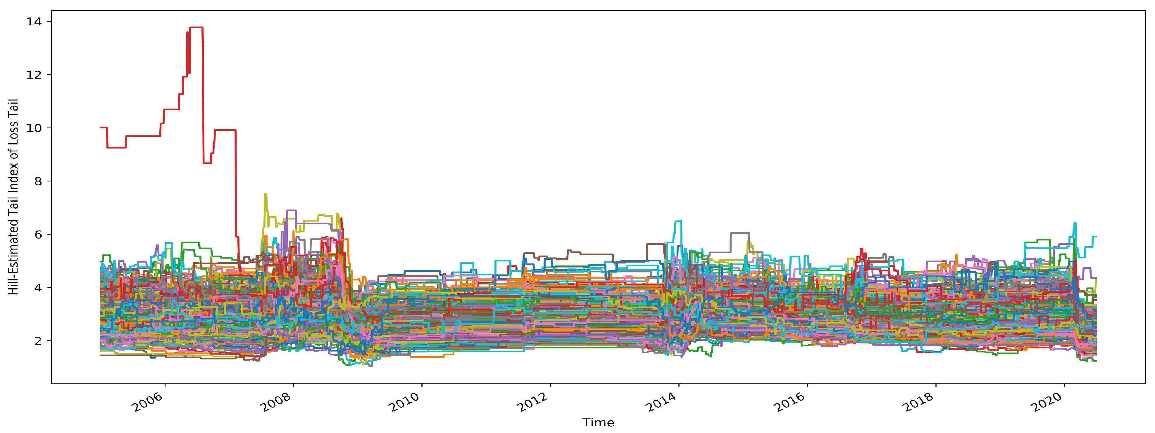
Lastly, we estimate the tail index of each stock by using the Hill estimator defined in (8) by using 5-year rolling window. That is, from 3 January 2005 to 29 June 2020, one every other day, the tail index of each stock is estimated using the previous 5-year alternate-day data. Figure 2 shows the estimates of all the stocks. Almost all tail indices fall significantly both in 2008–2009 and in 2020 as tails become heavier in response to extreme risk market movements.

4. Empirical Study

In this section, we examine the performance of the portfolio that minimizes the DR. It is also compared with other four strategies, EW, MV, ERI, and MDP, together with the S&P 500 index. We first carry out the analysis by assuming all the 361 stocks follow a MRV model. Then we group the stocks with similar tail indices and analyze the performances of the five strategies for each group. Before the empirical study, we discuss the estimation method for DR portfolio and the backtest method.
By fitting the stock losses with the MRV model, the DR portfolio is estimated using the method introduced in Section 2. To be more specific, we first calculate DR w , 1 using (4), which is the limit of DR w , q by letting q go to 1. The solution of minimizing DR w , 1 , w * , is used to approximate the DR portfolio w q . In the calculation of DR w , 1 , since only considering loss, η w is estimated by
η ^ w = 1 k w T S π ( j ) + α ^ .
The tail index α is estimated α ^ using (8). The proportion k is chosen to balance bias and variance of estimation. Here, we choose k as 4 % when estimating α . The spectral measure estimator Ψ ^ is given by (9), where k is 10 % .
We perform out-of-sample tests to examine the robustness of the DR strategy. The DR is minimized on a 5-year rolling window. The backtest period is from 3 January 2005 to 29 June 2020. The rolling window is moved on alternate days and the portfolio is rebalanced on alternate days as well. For example, on 3 January 2005, the optimal weights are calculated based on previous 630 observations (5 years before 3 January 2005). There are a total of 2021 rebalancing dates in the backtest period. To calculate portfolio weights, we deploy sequential least-squares programming methods given an equal weight ( 1 / d , 1 / d , , 1 / d ) initialization. We restrict to no short selling and thus all the weights are non-negative and in between 0 and 1. The error margin is set as 1 × 10 10 .

4.1. Analysis for All Stocks

We first carry out our analysis on all 361 stocks. When we apply the DR or ERI strategies, we fit the 361 stocks into a MRV model. This is a very rough fitting but some interesting results can be obtained. In the next subsection, a finer fitting is carried out for subgroups of the 361 stocks. This approach was also used in Mainik et al. (2015).
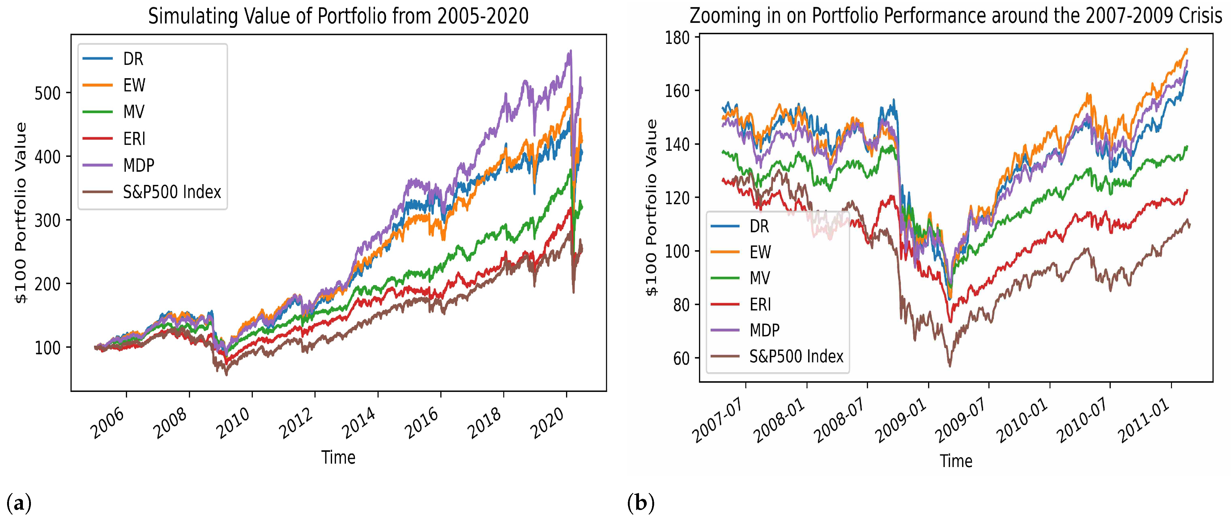
The portfolio values under all five strategies (DR, EW, MV, ERI, and MDP) together with S&P 500 index in the backtest period are plotted in Figure 3. Although not directly implied by our theoretical results, the DR strategy overall has the highest portfolio value, especially during the financial crisis of 2007–2009 period and 2020 stock market crash due to the COVID-19 pandemic.
In Table 2, we further compare the performance of the five strategies from different aspects. Subsequently, we discuss them individually.
The cumulative return (CR) is return over entire backtest period from 3 January 2005 to 29 June 2020 with alternate-day rebalancing. The annualized return (AR) annualizes CR by counting 126 alternate trading days in a year, and AR is calculated as
A R = ( 1 + C R ) 126 2021 1 .
As seen from Figure 3, with no surprise, the DR portfolio has higher CR and AR than the rest.
The Sharpe ratio is estimated by using the sample mean and sample variance for the alternate-day rebalanced portfolios. Since the risk-free return rate r f is both difficult to estimate and close to 0, we approximate r f = 0 for calculations. In Table 2, the annualized Sharpe ratio is reported, which is approximated by multiplying the alternate-day Sharpe ratio with 126 . The MDP portfolio has the highest Sharpe ratio among all of the five strategies and this is much expected as MDP is diversifying away risks measured by the variance, which is the same measure used in the Sharpe ratio. Since our focus here is on extreme risks, standard deviation is not a good risk measure in this case. A modification of the Sharpe ratio, by replacing the standard deviation with Expected Shortfall (ES) risk measure, is better to capture extreme risks and hence a good performance metric in this context. More specifically, this modified Sharpe ratio, called STARR p ( Z ) , is defined as
STARR p ( Z ) = E ( Z r f ) ES p ( Z r f ) ,
where Z is the portfolio return and r f is risk-free rate; see e.g., Rachev et al. (2005). We let r f = 0 and ES p is the expected shortfall risk measure at confidence level p ( 0 , 1 ) . In empirical studies, we take p = 95 % . The ES of a loss Z is estimated as
ES ^ 0.95 ( Z ) = 1 2020 × 5 % i = 0 2020 × 5 % 1 Z ( n i )
where Z ( n ) Z ( n 1 ) Z ( 1 ) are the order statistics. The annualized STARR ratio, reported in Table 2, is obtained by multiplying alternate-day STARR ratio with 126 . DR has the highest annualized STARR ratio.
Maximum drawdown assesses relative riskiness of one strategy versus another. A low maximum drawdown indicate losses from investment were small. DR has a lower drawdown than EW, MDP, and the index. ERI having the lowest maximum drawdown is somewhat expected as it, by definition, minimizes aggregate risks of the portfolio.
Concentration coefficient (CC) for a strategy at time t is defined as
CC t = 1 | | w t | | 2 2 ,
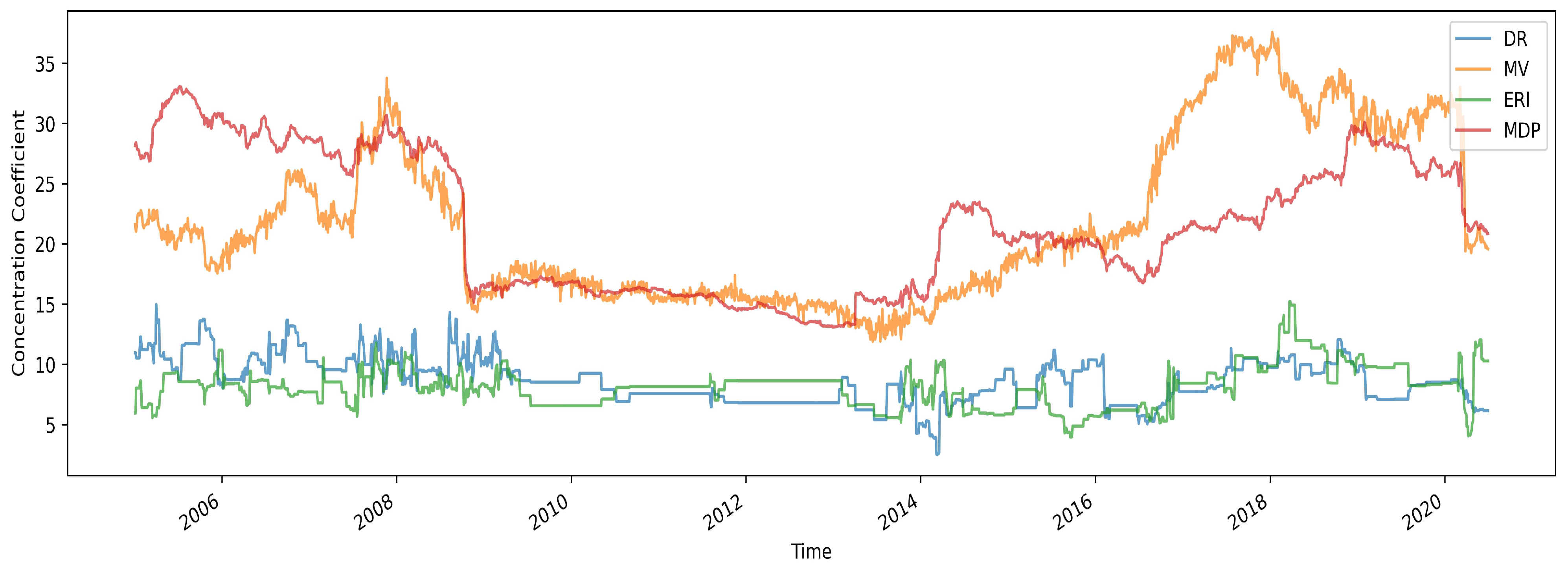
where w t is the optimal portfolio weights. For equally weighted portfolios, CC is maximized. When a portfolio concentrates on fewer stocks, the value of CC decreases. While CC ignores correlations in exposures, it is effective to capture risk appetite and stress levels with low computational complexity. In Figure 4, CC is plotted for DR, MV, ERI, and MDP in the backtest period. Both DR and ERI have very low CCs over time and are very stable. MV and MDP have high CCs over the financial crisis of 2007–2009 and around 2018. This shows that the selection of stocks are related to the choices of the risk measures: especially during the crisis time, strategies (MV and MDP) using variance as the risk measure need more stocks to diversify away the risk while strategies (DR and ERI) using VaR need fewer stocks. The average CC over the backtest period is calculated for each strategy shown in Table 2. Again, DR and ERI have similar but small CC suggesting they are selective in stocks.
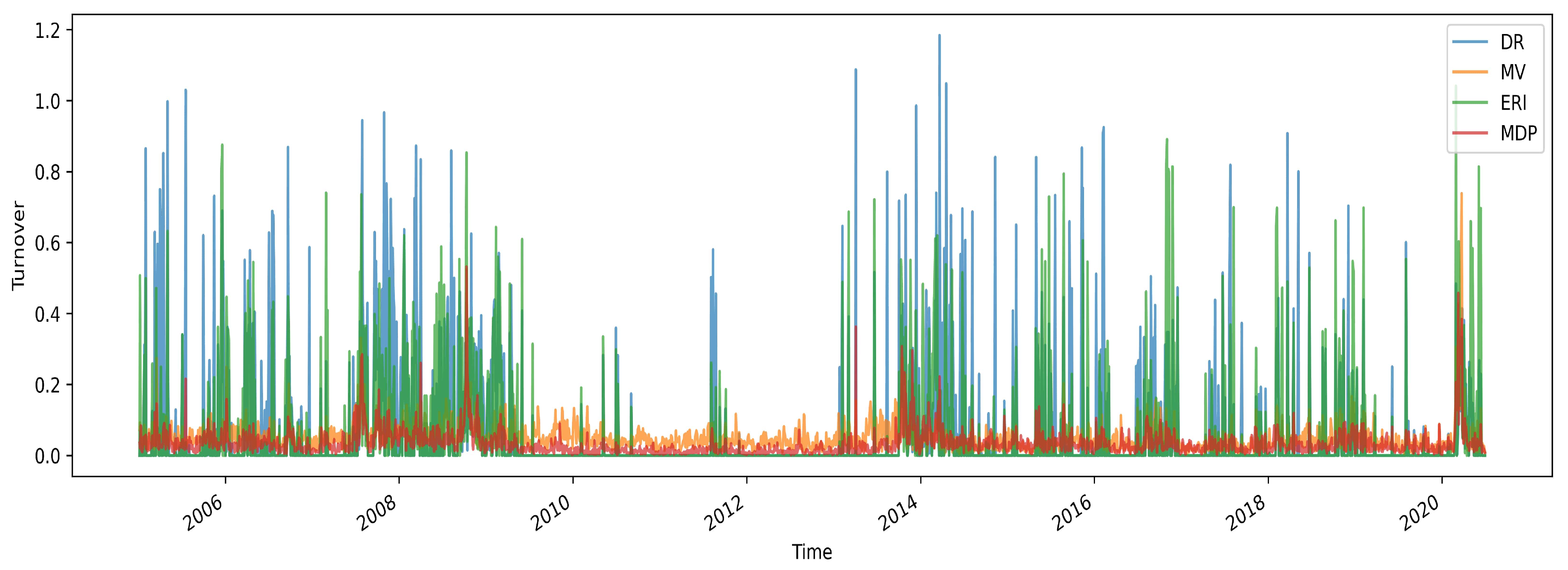
The portfolio turnover is defined as τ t = | | w t w t 1 | | 1 where w t is the optimal portfolio weights. Turnover captures extent of re-balancing at each time-stamp by proxy on change in weights vector, and evaluates transaction costs of a strategy. In Figure 5, the turnovers are plotted for DR, MV, ERI, and MDP in the backtest period. The average of turnover for each strategy is reported Table 2. Both DR and ERI have higher turnover than other strategies.
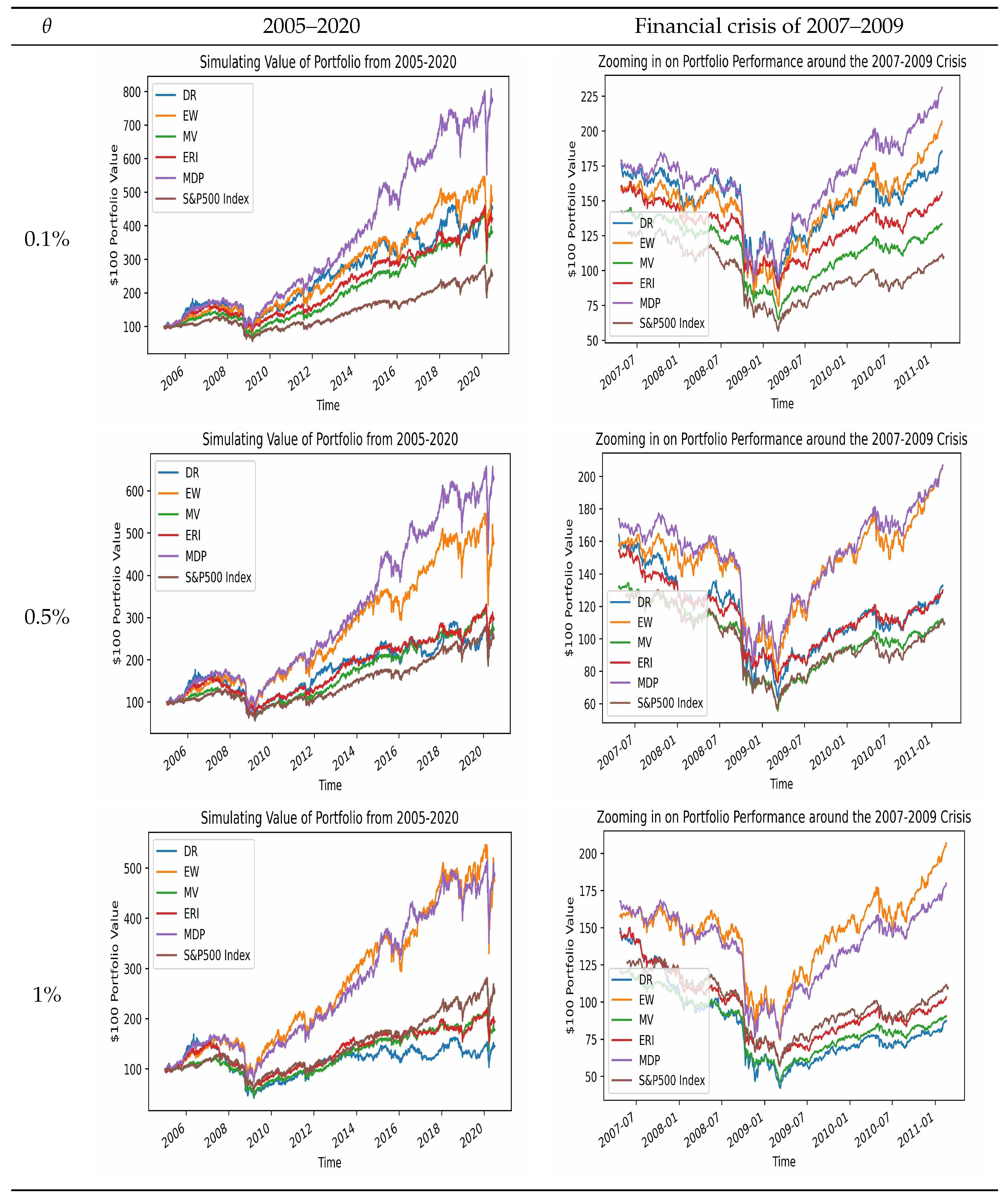
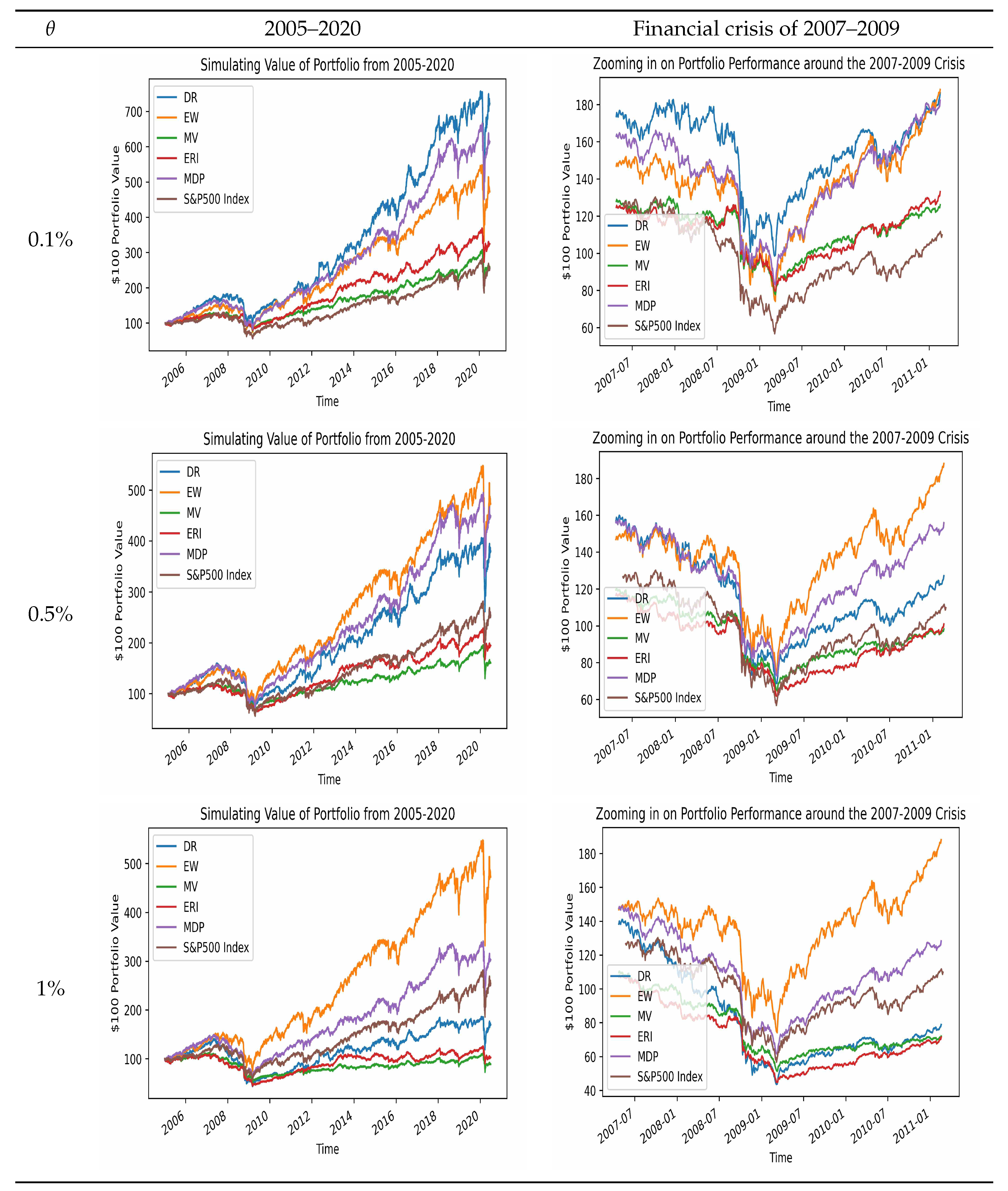
From the above analysis, the VaR-based strategies (DR and ERI) have high turnover compared to the variance-based strategies (MV and MDP). This may be due to that VaR is more sensitive to extreme risks as opposed to variance taking both profits and losses into account. At the same time, DR and ERI have very low CCs, which means these strategies consist of fewer stocks. Thus, next we add the transaction cost to see if how low CC and high turnover affect the performance of these strategies. According to Wrobel (2017), from April 2007 to August 2008 the transaction cost increased 37.6 % and from August to October in 2008 the transaction cost increased 26.9 % , which is the highest levels in 5 years. That is the transaction cost during the financial crisis of 2007–2009 is higher than the normal time. For simplicity, we assume a constant transaction cost: the transaction cost per dollar amount traded is θ during normal time, and the cost during the crisis time is θ f c = 1.5 θ . That is the transaction cost is one and a half times of that in the normal time. Let θ = 0.1 % , 0.5 % , 1 % . The cumulative return with transaction cost is reported in Table 2 and the corresponding portfolio values are shown in Figure 6. When the transaction cost is as low as θ = 0.1 % , DR still outperforms other strategies due to its low CC. Once the transaction cost is higher ( θ = 0.1 % , 0.5 % , 1 % ), EW has the best performance and DR has the moderate performance because of its high turnover.
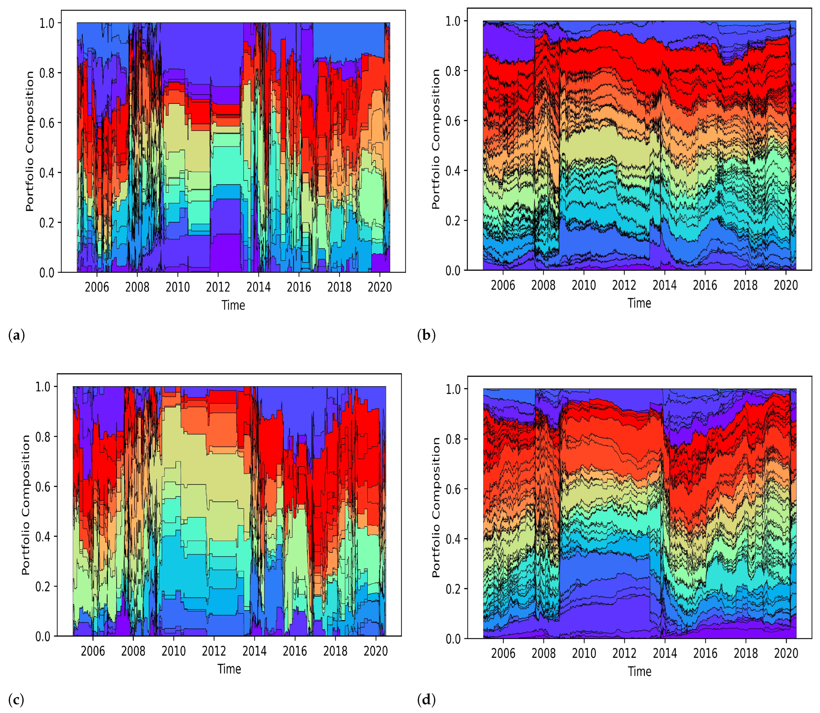
We further plot the optimal weights for DR, MV, ERI, and MDP at each rebalancing date during the backtest period in Figure 7. The patterns of the optimal weights reinforce the observations in the study of the CC and turnover that DR and ERI consist of fewer stocks and have more significant changes in composition. They have similar patterns, i.e., frequent large changes in stock composition during crises (2008 financial crisis and 2020 stock market crash) and rather stable otherwise, while MV and MDP exhibit frequent but small changes in composition throughout. This difference should be attributed to the choice of risk measure. VaR is a measure to capture extreme risks better than variance so that both DR and ERI strategies are more sensitive in the crisis time, where extreme risks occur.
To analyze the degree of diversification, we perform principal component analysis (PCA) for each strategy. The first principal component is calculated on the weighted returns, that is for a 2021 × 361 matrix M, with
M [ i , j ] = w i * ( j ) X i ( j )
where w i * ( j ) is the optimal weight and X i ( j ) is the log-return of the jth stock at time i. To account for temporal changes, we compute percentage of the sample variance explained by the first principal component on the first i rows of the matrix M at each time point i = 1 , 2 , , 2021 in the backtest period. The estimated percentage of variance is plotted over time in Figure 8. We report the last percentage ( i = 2021 ) in Table 2. The smaller this value the greater the diversification. ERI has almost the smallest percentage of sample variance explained by the first principal component for majority of the time as showed in Figure 8 and the smallest average value among all strategies although it has a low concentration coefficient. DR shows the smallest percentage after the 2008 crisis started. Similar pattern can be expected for the COVID-19 pandemic period. Although complete performance of the strategies over the pandemic are not shown here due to the time range of data, still we can conclude that DR is efficient in diversifying extreme risks and thus a feasible strategy in the period of a crisis.
The skewness and kurtosis of portfolio returns are reported as well. DR has a right skew while all the benchmark strategies have left skews. DR also has the highest kurtosis. This reinforces the findings in cumulative return and annualized returns that DR has the ability to generate higher risk-adjusted returns.
We ascertain DR’s distinctness with DR weights’ cosine similarity and DR returns’ Pearson correlation coefficient against other strategies in Table 3. We observe low cosine similarities on DR weights coupled with high correlation on returns with other strategies. This dichotomy reinforces DR’s novelty in portfolio allocation since correlated returns hint at it capitalizing on similar temporal market movements as other strategies, while dissimilar weights (and higher returns) suggest it does so with an effective distinctive methodology.

4.2. Analysis of Grouped Stocks

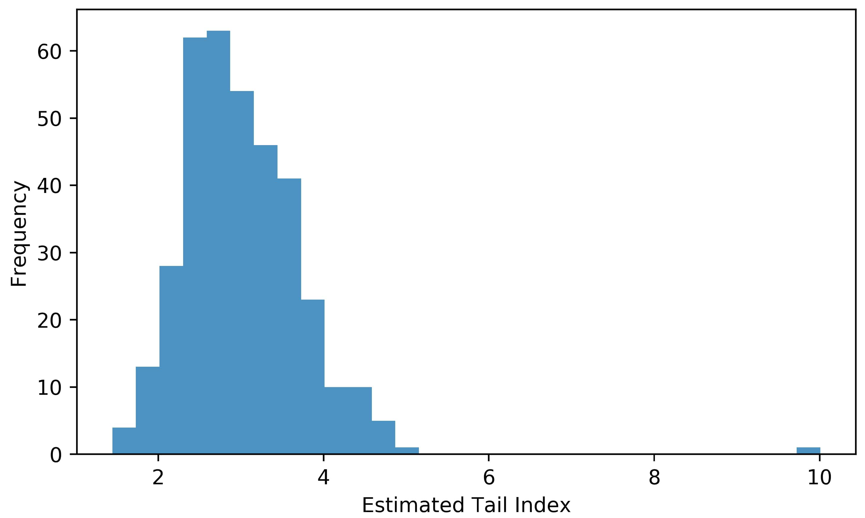
In the previous section, all 361 stocks are fitted into a MRV model. In this subsection, we consider portfolios of stocks grouped with similar tail indices. Figure 9 shows the distribution of the tail indices calculated by Hill estimator based on a 5-year window of alternate-day data from 1 January 2000 to 31 December 2004 for all 361 stocks. We divide these stocks into three buckets as shown in Table 4.
The group of stocks with tail indices α 2.5 contains the most heavy-tailed securities. The portfolio values for each strategy are plotted in Figure A1 in Appendix A. The portfolio values with transaction costs are plotted in Figure A2. The performance of each strategy for this group of stocks is reported in Table A1. DR has the moderate performance in returns. When the transaction cost is included, DR has low returns among the five strategies but it is still higher than ERI. DR has the lowest average percentage of sample variance explained by the first principal component. This shows that DR has highest significant effect of diversification for the most heavy-tailed stocks.
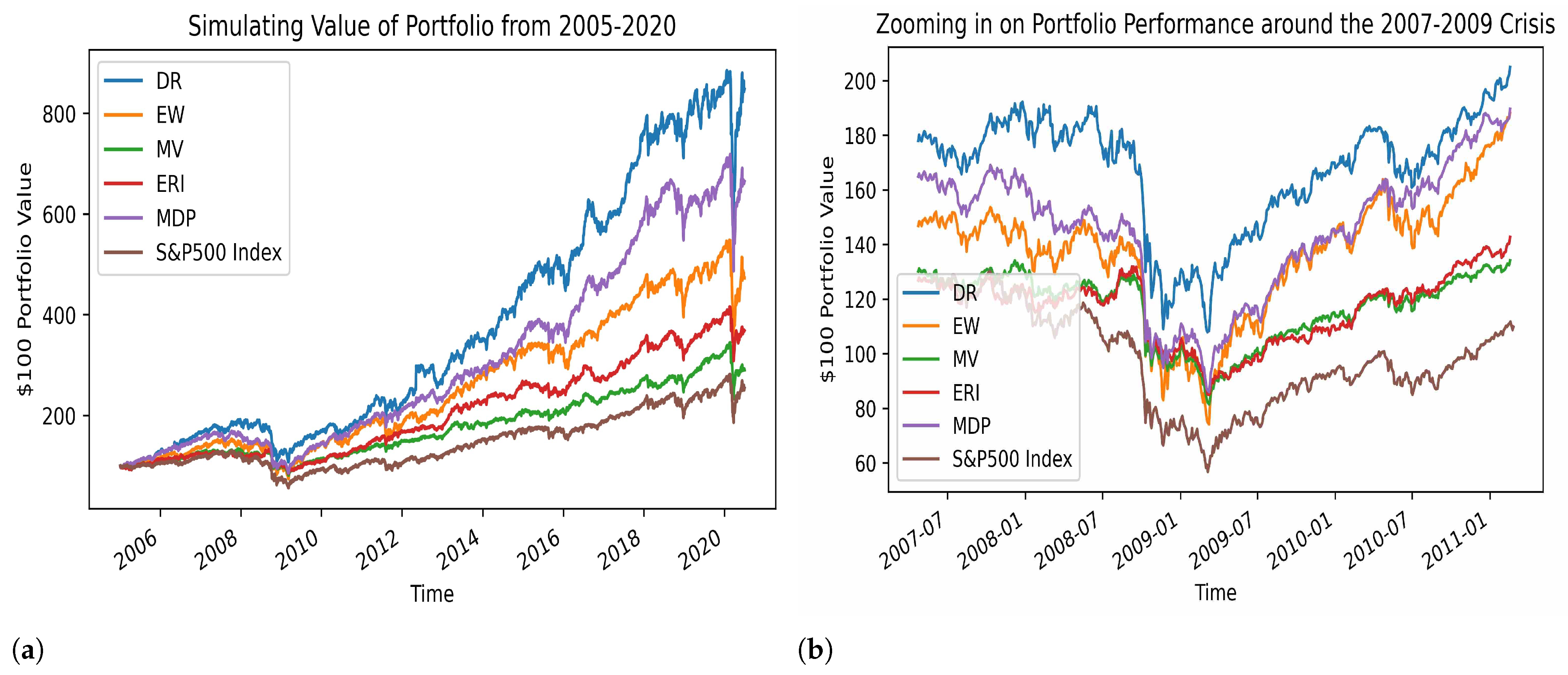
The group of stocks with tail indices 2.5 < α 3.5 is by far the largest, with 195 listed securities. The portfolio values for each strategy are plotted in Figure A3; the portfolio values with transaction costs are plotted in Figure A4. The performance is reported in Table A2. DR performs similar to that of the entire 361 stocks: it has highest cumulative return, annualized return, Sharpe ratio, STARR, and lowest average percentage of sample variance explained by the first principal component. When the transaction cost is low ( θ = 0.1 % ), DR still has the highest return rate due to low CC; however, when the transaction cost is higher, DR has moderate performance due to high turnover. This shows that DR works well for a vast majority of our securities universe.
The group of stocks with tail indices α > 3.5 contains the most light-tailed stocks. The portfolio values for each strategy are plotted in Figure A5 and the portfolio values with transaction costs are plotted in Figure A6. The performance is reported in Table A3. Again, DR has the lowest average percentage of sample variance explained by the first principal component, reflecting the most significant effect of diversification. When transaction cost presents, DR has moderate performance.
To summarize, DR has highest effect of diversification in all three groups of stocks. It performs the best for most of the stocks with tail indices 2.5 < α 3.5 .

5. Conclusions

In this paper, we empirically test the performance of a portfolio optimization strategy that minimizes DR on S&P 500 stocks. The performance is compared with benchmark strategies: EW, MV, ERI, and MDP. The DR and MDP strategies have similar structure of capturing the degree of diversification but using VaR and variance as the risk measure, respectively. ERI and MV are strategies that minimize risks, which are measured by VaR and variance, respectively. DR and ERI, both using VaR as the risk measure, are very selective in stocks and have high turnovers. This implies that strategies based on VaR have major changes in stock compositions during the crisis time, highlighting high sensitivity to extreme risks. When there is no transaction cost or low transaction cost, DR shows promising cumulative return, annualized return, Sharpe ratio, and STARR at 95 % . In addition, it showcases the highest unfaltering level of diversification when the strategy is performed for the entire stock universe during the crisis time and for grouped stocks with similar tail indices over the entire test period.
Our study shows the importance of analyzing diversification benefit based on measures for extreme risks in portfolio optimization. In the data range analyzed, the DR strategy outperformed other strategies by diversifying more risks away and maintaining a good level of return during the crisis times, both 2007–2009 global financial crisis and the COVID-19 pandemic. Moreover, the DR strategy is invariant from using different quantile-based risk measures in the definition of DR (2), such as ES and expectiles, which means it does not suffer from the drawbacks of VaR. Thus, the DR strategy can be applied when extreme risks present in the market, that is when stronger interconnectedness is shown among the stocks and some stocks show sharp declines in prices. The current analysis is built upon the assumption that the underlying risks can be modeled by the MRV. Due to the difficulty of verifying the MRV model for high dimensional data, the proposed model (MRV) may not be appropriate to be applied in the entire stock market. For future research, flexible high dimensional models that can capture extreme risks should be investigated to see if the DR strategy can still have good performance during the crisis times. Another drawback of the current DR strategy is that it only extracts the most diversification benefit; that is, only the downside risk is minimized. This may be the reason that the DR strategy performs well during the crisis time but not as good as some other strategies in the normal time. For future work, strategies that can achieve higher return and also maintain the most diversification benefit may perform equally well during the crisis and the normal time, which is of great importance to study.

Author Contributions

Conceptualization, F.Y.; methodology, F.Y.; formal analysis, N.J.M. and F.Y.; data curation, N.J.M.; writing—original draft preparation, N.J.M. and F.Y.; writing—review and editing, F.Y.; supervision, F.Y.; funding acquisition, F.Y. All authors have read and agreed to the published version of the manuscript.

Funding

This research was funded by the grant from the Natural Sciences and Engineering Research Council of Canada of grant number 04242.

Acknowledgments

We thank the Editor and anonymous referees for their thoughtful comments which greatly helped improving the paper.

Conflicts of Interest

The authors declare no conflict of interest.

Appendix A

Appendix A.1. Proof

Proof of Theorem 1.
By Theorem 4.5(a) of Mainik and Rüchendorf (2010), the estimators η ξ j for 1 j d + 1 satisfies that
k η ^ ξ j η ξ j w B Ψ f ξ j , α + b ξ j + c j Y .
Note that DR w can be rewritten as
DR w , 1 = h η w , η e 1 , , η e d .
The gradient of h is
h = h x i 1 i d + 1 = 1 / α x 1 1 / α 1 i = 2 d + 1 w i x i 1 / α , 1 / α w 1 x 1 1 / α x 2 1 / α 1 i = 2 d + 1 w i x i 1 / α 2 , .
The Hessian matrix of h is
2 h = 2 h x i x j 1 i , j d + 1 ,
where
2 h 2 x 1 = 1 / α ( 1 / α 1 ) x 1 1 / α 2 i = 2 d + 1 w i x i 1 / α ,
for 2 i d + 1
2 h 2 x i = 1 / α ( 1 / α 1 ) w i 1 x 1 1 / α x i 1 / α 2 j = 2 d + 1 w i x j 1 / α 2 + 1 / α 2 w i 1 2 x 1 1 / α x i 2 / α 2 j = 2 d + 1 w i x j 1 / α 4 ,
and
2 h x 1 x i = 1 / α 2 w i x 1 1 / α 1 x i 1 / α 1 j = 2 d + 1 w i x j 1 / α 2 ,
and for 2 i j d + 1
2 h x i x j = 1 / α 2 w i 1 w j 1 x 1 1 / α x i 1 / α 1 x j 1 / α 1 i = 2 d + 1 w i x i 1 / α 4 .
By the Taylor expansion, for x , y ( 0 , 1 ] d + 1 and y t y , we have for t > 0 ,
h x + t y t h ( x ) t h ( x ) y t t y t T 2 h ( x ) y t + o ( t 2 ) .
Since i = 2 d + 1 w i x i 1 / α is bounded away from 0 and x i 1 / α 2 < for any x i ( 0 , 1 ] , Hessian matrix 2 h ( x ) < . Hence,
h x + t y t h ( x ) t h ( x ) y 0 , as t 0 and y t y
That is, the function h is Hadamard differentiable. By the functional delta method (e.g., Theorem 20.8 in Van der Vaart (2000)), the desired result follows. □

Appendix A.2. Tables and Figures

The followings are figures and tables from Section 4.2.
Figure A1. Portfolio values for grouped stocks with tail indices α 2.5 . (a) Portfolio with α 2.5 in the entire backtest period; (b) portfolio with α 2.5 in the crisis period.
Risks 10 00101 g0a1
Table A1. Performance comparisons for DR, EW, MV, ERI, MDP, and S&P 500 index for stocks with α 2.5 .
MetricDREWMVERIMDPS&P 500
Cumulative return305.59%324.20%219.87%154.42%406.11%154.00%
Annualized return9.12%9.43%7.52%5.99%10.64%5.98%
Annualized Sharpe ratio0.59410.60700.62790.49280.72590.2849
Annualized STARR 0.95 0.25120.24690.26010.20480.30280.1139
Maximum drawdown47.69%46.62%38.06%42.21%41.22%56.78%
Concentration coefficient8.155884.000013.16167.142018.2519N/A
Average turnover0.05900.00000.04740.04500.0279N/A
CR with θ = 0.1 % 252.50%324.20%187.16%129.16%374.40%N/A
CR with θ = 0.5 % 100.97%324.20%86.49%50.77%266.19%N/A
CR with θ = 1 % −0.62%324.20%8.70%−10.76%164.92%N/A
PCA11.27%38.34%28.32%17.65%14.74%N/A
Skewness−0.2476−0.1166−0.8514−0.8160−0.4977−0.2556
Kurtosis8.42348.779211.618010.58317.030813.9341
Figure A2. Portfolio values with transaction cost for grouped stocks with tail indices α 2.5 when θ = 0.1 % , 0.5 % , 1 % , θ f c = 1.5 θ .
Risks 10 00101 g0a2
Figure A3. Portfolio values for grouped stocks with tail indices 2.5 < α 3.5 .
Risks 10 00101 g0a3
Table A2. Performance comparisons for DR, EW, MV, ERI, MDP, and S&P 500 index for stocks with 2.5 < α 3.5 .
MetricDREWMVERIMDPS&P 500
Cumulative return742.46%388.84%189.04%284.35%545.97%154.00%
Annualized return14.21%10.40%6.84%8.76%12.33%5.98%
Annualized Sharpe ratio0.85100.60350.59800.70960.82580.2849
Annualized STARR 0.95 0.36110.24770.24800.30460.34010.1139
Maximum drawdown46.62%52.52%38.50%42.16%51.96%56.78%
Concentration coefficient7.8232195.000016.40926.532118.6969N/A
Average turnover0.06970.00000.05270.04730.0321N/A
CR with θ = 0.1 % 618.14%388.84%157.13%244.67%500.34%N/A
CR with θ = 0.5 % 278.86%388.84%61.01%122.79%347.81%N/A
CR with θ = 1 % 70.01%388.84%−10.33%28.98%210.39%N/A
PCA8.94%39.19%25.99%19.34%15.75%N/A
Skewness−0.2755−0.0556−1.1798−0.5133−0.6143−0.2556
Kurtosis8.12607.737611.00684.58517.687713.9341
Figure A4. Portfolio values with transaction cost for grouped stocks with tail indices 2.5 < α 3.5 when θ = 0.1 % , 0.5 % , 1 % , θ f c = 1.5 θ .
Risks 10 00101 g0a4
Figure A5. Portfolio values for grouped stocks with tail indices α > 3.5 .
Risks 10 00101 g0a5
Table A3. Performance comparisons for DR, EW, MV, ERI, MDP, and S&P 500 index for stocks with α > 3.5 .
MetricDREWMVERIMDPS&P 500
Cumulative return414.42%375.12%314.14%356.74%714.50%154.00%
Annualized return10.75%10.20%9.26%9.93%13.97%5.98%
Annualized Sharpe ratio0.57350.55750.65580.66980.78610.2849
Annualized STARR 0.95 0.25050.23270.26830.28700.33260.1139
Maximum drawdown48.03%54.70%54.34%45.40%49.61%56.78%
Concentration coefficient6.643182.00009.71445.796813.1654N/A
Average turnover0.05100.00000.03760.03620.0221N/A
CR with θ = 0.1 % 353.40%375.12%280.57%319.34%673.63%N/A
CR with θ = 0.5 % 173.39%375.12%171.35%197.86%529.65%N/A
CR with θ = 1 % 45.01%375.12%77.77%94.07%386.70%N/A
PCA22.79%42.73%29.79%23.27%35.33%N/A
Skewness0.35350.0349−0.8981−0.3410−0.3370−0.2556
Kurtosis10.24207.620010.63074.93136.134513.9341
Figure A6. Portfolio values with transaction cost for grouped stocks with tail indices α > 3.5 when θ = 0.1 % , 0.5 % , 1 % , θ f c = 1.5 θ .
Risks 10 00101 g0a6

References

  1. Acharya, Viral V., Lasse H. Pedersen, Thomas Philippon, and Matthew Richardson. 2017. Measuring systemic risk. The Review of Financial Studies 30: 2–47. [Google Scholar] [CrossRef]
  2. Billio, Monica, Mila Getmansky, Andrew W. Lo, and Loriana Pelizzon. 2012. Econometric measures of connectedness and systemic risk in the finance and insurance sectors. Journal of Financial Economics 104: 535–59. [Google Scholar] [CrossRef]
  3. Chen, Hua, John Cummins, Krupa Viswanathan, and Mary Weiss. 2014. Systemic risk and the interconnectedness between banks and insurers: An econometric analysis. Journal of Risk and Insurance 81: 623–52. [Google Scholar] [CrossRef]
  4. Choo, Weihao, and Piet de Jong. 2010. Determining and allocating diversification benefits for a portfolio of risks. ASTIN Bulletin 40: 257–69. [Google Scholar] [CrossRef]
  5. Choueifaty, Yves, and Yves Coignard. 2008. Toward maximum diversification. The Journal of Portfolio Management 35: 40–51. [Google Scholar] [CrossRef] [Green Version]
  6. Cui, Hengxin, Ken Seng Tan, and Fan Yang. 2021. Diversification in catastrophe insurance markets. ASTIN Bulletin: The Journal of the IAA 51: 753–78. [Google Scholar] [CrossRef]
  7. Cui, Hengxin, Ken Seng Tan, Fan Yang, and Chen Zhou. 2022. Asymptotic Analysis of Portfolio Diversification. Available online: https://uwaterloo.ca/scholar/sites/ca.scholar/files/f66yang/files/dr.pdf (accessed on 28 March 2022).
  8. Degen, Matthias, Dominik D. Lambrigger, and Johan Segersigger. 2010. Risk concentration and diversification: Second-order properties. Insurance: Mathematics and Economics 46: 541–46. [Google Scholar] [CrossRef] [Green Version]
  9. Embrechts, Paul, Dominik D. Lambrigger, and Mario V. Wüthrich. 2009. Multivariate extremes and the aggregation of dependent risks: Examples. Extremes 12: 107–27. [Google Scholar] [CrossRef] [Green Version]
  10. Gabaix, Xavier, Parameswaran Gopikrishnan, Vasiliki Plerou, and H. Eugene Stanley. 2003. A theory of power-law distributions in financial market fluctuations. Nature 423: 267–70. [Google Scholar] [CrossRef]
  11. Gorton, Gary B. 2008. The Panic of 2007. Technical Report. Cambridge: National Bureau of Economic Research. [Google Scholar]
  12. Hamidieh, Kamal, Stilian Stoev, and George Michailidis. 2009. On the estimation of the extremal index based on scaling and resampling. Journal of Computational and Graphical Statistics 18: 731–55. [Google Scholar] [CrossRef] [Green Version]
  13. Hill, Bruce M. 1975. A simple general approach to inference about the tail of a distribution. The Annals of Statistics 3: 1163–74. [Google Scholar] [CrossRef]
  14. Huang, Xin, Hao Zhou, and Haibin Zhu. 2009. A framework for assessing the systemic risk of major financial institutions. Journal of Banking & Finance 33: 2036–49. [Google Scholar]
  15. Huang, Xin, Hao Zhou, and Haibin Zhu. 2012. Assessing the systemic risk of a heterogeneous portfolio of banks during the recent financial crisis. Journal of Financial Stability 8: 193–205. [Google Scholar] [CrossRef] [Green Version]
  16. Hüsler, Jürg, and Deyuan Li. 2006. On testing extreme value conditions. Extremes 9: 69–86. [Google Scholar] [CrossRef] [Green Version]
  17. Jansen, Dennis W., and Casper G. de Vries. 1991. On the frequency of large stock returns: Putting booms and busts into perspective. The Review of Economics and Statistics 73: 18–24. [Google Scholar] [CrossRef] [Green Version]
  18. Leadbetter, Malcolm Ross, Georg Lindgren, and Holger Rootzén. 2012. Extremes and Related Properties of Random Sequences and Processes. New York: Springer Science & Business Media. [Google Scholar]
  19. Longin, François M. 1996. The asymptotic distribution of extreme stock market returns. The Journal of Business 69: 383–408. [Google Scholar] [CrossRef]
  20. Loretan, Mico, and Peter C. B. Phillips. 1994. Testing the covariance stationarity of heavy-tailed time series: An overview of the theory with applications to several financial datasets. Journal of Empirical Finance 1: 211–48. [Google Scholar] [CrossRef]
  21. Mainik, Georg, Georgi Mitov, and Ludger Rüchendorf. 2015. Portfolio optimization for heavy-tailed assets: Extreme risk index vs. markowitz. Journal of Empirical Finance 32: 115–34. [Google Scholar] [CrossRef] [Green Version]
  22. Mainik, Georg, and Ludger Rüchendorf. 2010. On optimal portfolio diversification with respect to extreme risks. Finance and Stochastics 14: 593–623. [Google Scholar] [CrossRef] [Green Version]
  23. Mao, Tiantian, and Fan Yang. 2015. Risk concentration based on expectiles for extreme risks under fgm copula. Insurance: Mathematics and Economics 64: 429–39. [Google Scholar] [CrossRef]
  24. McCulloch, J. Huston. 1997. Measuring tail thickness to estimate the stable index α: A critique. Journal of Business & Economic Statistics 15: 74–81. [Google Scholar]
  25. McNeil, Alexander J. 1998. Calculating Quantile Risk Measures for Financial Return Series Using Extreme Value Theory. Technical Report. Zürich: ETH Zurich. [Google Scholar]
  26. Rachev, Svetlozar T., Christian Menn, and Frank J. Fabozzi. 2005. Fat-Tailed and Skewed Asset Return Distributions: Implications for Risk Management, Portfolio Selection, and Option Pricing. New York: John Wiley & Sons, vol. 139. [Google Scholar]
  27. Richardson, Matthew, and Tom Smith. 1993. A test for multivariate normality in stock returns. The Journal of Business 66: 295–321. [Google Scholar] [CrossRef]
  28. Rivera-Escobar, Orlando, John Willmer Escobar, and Diego Fernando Manotas. 2022. Measurement of systemic risk in the colombian banking sector. Risks 10: 22. [Google Scholar] [CrossRef]
  29. Schnieper, Rene. 2000. Portfolio optimization. ASTIN Bulletin 30: 195–248. [Google Scholar] [CrossRef] [Green Version]
  30. Van der Vaart, Aad W. 2000. Asymptotic Statistics. Cambridge: Cambridge University Press. [Google Scholar]
  31. Wrobel, Jason. 2017. The cost of crisis: Why stock fees rise when markets slip. In Beyond the Numbers: Prices and Spending; Washington, DC: U.S. Bureau of Labor Statistics, February, vol. 6. Available online: https://www.bls.gov/opub/btn/volume-6/cost-of-crisis.htm (accessed on 28 March 2022).
Figure 1. Estimates of extremal index for stock losses with different frequencies. (a) Daily losses; (b) alternate-day losses; (c) weekly losses.
Risks 10 00101 g001
Figure 2. Tail indices estimated by Hill estimator for 361 S&P500 stocks.
Risks 10 00101 g002
Figure 3. The values of portfolios of 361 stocks under the strategies of DR, EW, MV, ERI, and MDP, and the values of S&P 500 index. The initial value for each portfolio is set as $100. (a) The entire backtest period 2005–2020; (b) the financial crisis of 2007–2009 period.
Risks 10 00101 g003
Figure 4. CC of DR, MV, MDP, and ERI for the 361-stock portfolio over the backtest period.
Risks 10 00101 g004
Figure 5. Turnover of DR, MV, MDP, and ERI for the 361-stock portfolio over the backtest period.
Risks 10 00101 g005
Figure 6. Portfolio value of 361 stocks with transaction cost θ = 0.1 % , 0.5 % , 1 % and θ f c = 1.5 θ .
Risks 10 00101 g006
Figure 7. Optimal weights under the strategies DR, MV, ERI, and MDP for the 361-stock portfolio over the backtest period. (a) DR; (b) MV; (c) ERI; (d) MDP.
Risks 10 00101 g007
Figure 8. Percentage of variance explained by first principal component for 361-Stock portfolio over the backtest period.
Risks 10 00101 g008
Figure 9. Distribution of tail indices of all 361 stocks.
Risks 10 00101 g009
Table 1. Number of stock falls in p-value intervals for exploratory analysis.
p-Value IntervalLB-Q(5)Co-SkewnessCo-KurtosisPE
( 0 , 0.001 ] 144316293115
( 0.001 , 0.01 ] 6271864
( 0.01 , 0.05 ] 668861
( 0.05 , 0.1 ] 267829
( 0.1 , 0.3 ] 28101350
( 0.3 , 1.0 ] 35122042
Table 2. Performance comparisons for DR, EW, MV, ERI, MDP, and S&P 500 index for the 361-stock portfolio.
MetricDREWMVERIMDPS&P 500
Cumulative return (CR)747.92%373.02%190.77%268.63%564.54%154%
Annualized return14.26%10.17%6.88%8.47%12.53%5.98%
Annualized Sharpe ratio0.82030.59740.60570.69860.84230.2849
Annualized STARR 0.95 0.36170.24520.24980.29180.35780.1139
Maximum drawdown43.79%51.64%39.15%35.51%49.08%56.78%
Concentration coefficient8.6449361.000021.89088.132921.7522N/A
Average turnover0.06790.00000.051760.05430.0343N/A
CR with θ = 0.1 % 622.21%373.02%158.30%224.51%514.36%N/A
CR with θ = 0.5 % 279.76%373.02%60.83%94.77%348.74%N/A
CR with θ = 1 % 69.71%373.02%−11.06%2.76%202.96%N/A
PCA28.96%39.39%20.13%14.19%22.44%N/A
Skewness0.6555−0.0494−1.1730−0.7705−0.6376−0.2556
Kurtosis14.35807.994711.48146.20757.898113.9341
Table 3. Comparing DR to benchmarks.
MetricEWMVERIMDP
Cosine Similarity [−1, 1]0.15383470.18626690.24480100.4276556
Correlation Coefficient [−1, 1]0.80417640.76971900.73143040.8724533
Table 4. Number of stocks across groupings.
Tail Index GroupingsNumber of Stocks
α 2.5 84
2.5 < α 3.5 195
3.5 < α 82
Publisher’s Note: MDPI stays neutral with regard to jurisdictional claims in published maps and institutional affiliations.