Article

Unit-Linked Tontine: Utility-Based Design, Pricing and Performance †

1
Institute of Insurance Science, University of Ulm, Helmholtzstrasse 20, 89069 Ulm, Germany
2
École d’Actuariat, Université Laval, 2425, rue de l’Agriculture, Quebec, QC G1V 0A6, Canada
*
Author to whom correspondence should be addressed.
An earlier version of this article is a part of the dissertation of Thorsten Sehner which is published on the Open Access Repository of Ulm University and Ulm University of Applied Sciences.
Risks 2022, 10(4), 78; https://doi.org/10.3390/risks10040078
Submission received: 27 January 2022 / Revised: 23 March 2022 / Accepted: 29 March 2022 / Published: 7 April 2022
(This article belongs to the Special Issue Actuarial Mathematics and Risk Management)

Abstract

:
Due to the low demand for conventional annuities, alternative retirement products are sought. Quite recently, tontines have been frequently brought up as a promising option in this respect. Inspired by unit-linked life insurance and retirement products, we introduce unit-linked tontines in this article, where the tontine payoffs are directly linked to the development of the underlying financial market. More specifically, we consider two different tontine payoff structures differing in the (non-)inclusion of guaranteed payments. We first price the unit-linked tontines by using the risk-neutral pricing approach. Consequently, we study the attractiveness of these products for a utility-maximizing policyholder and compare them with non-unit-linked tontines. Our numerical analysis sheds light on the design challenges and gives explanations why similar products might not be widely adopted already.

1. Introduction

Unit-linked insurance policies belong to the most frequently concluded contracts in the life insurance sector; for example, more than 50% of the UK life (re)insurance gross written premiums were attributed to the index- and unit-linked insurance field in 2019 according to Statista (2020b). Among other attractive features, higher return expectations, flexibility, design possibilities and tax advantages (see, e.g., Schiereck et al. 2020) certainly play a driving role in the attractiveness of these policies. Interesting subject areas related to unit-linked insurance contracts, such as variable annuities, include pricing and valuation from the insurer’s or the customers’ perspective (see, e.g., Aase and Persson 1994; Ekern and Persson 1996; Gatzert et al. 2011), hedging strategies (see, e.g., Møller 1998), impact of stochastic interest rates (see, e.g., Schrager and Pelsser 2004) or guarantee components (see, e.g., Ledlie et al. 2008). In this paper, inspired by variable annuities, we design and investigate a new type of tontine that is directly linked to the developments in the financial market.
Yet, why is it even reasonable to consider tontines when dealing with old-age provision? From a theoretical point of view, actuarially fairly priced annuities should actually be regarded favorably by rational customers (see, e.g., Peijnenburg et al. 2016; Yaari 1965). However, annuitization rates are rather low in reality (see, e.g., Hu and Scott 2007). This adverse phenomenon known as the annuity puzzle (see, e.g., Ramsay and Oguledo 2018) is hitting conventional annuities. Moreover, due to low interest rate environments and tightening solvency regulations, it is hard to expect that annuitization rates will go up any time soon. Therefore, alternative retirement products are naturally searched by insurers and customers, which brings up tontines as an option. Due to the backdrop of the demographic change (see, e.g., Margaras 2019), the so-called tontine retirement investment has become more and more important (see, e.g., Milevsky and Salisbury 2015; Sabin 2010). A main characteristic of tontines is that, in contrast to annuities, longevity risk is borne, to a great extent, by the pooled policyholders themselves. Hence, tontines are normally cheaper and, thus, potentially more attractive. Further discussions on practicalities, qualitative regulatory, technological and risk management issues associated with a tontine product can be found in Milevsky et al. (2018); Winter and Planchet (2021).
Let us briefly mention some of the recent literature that has addressed relevant topics related to tontine products. A general and historical view on tontines, as well as their possible applications for retirement income planning, is given in Milevsky (2015). Specific forms for the tontine payout structure are discussed in, e.g., Milevsky and Salisbury (2015). The question regarding how the tontine principle can be used to create tontine pensions for employees is studied in Forman and Sabin (2015). In Gemmo et al. (2020), investment possibilities in both tontines and traditional financial assets are investigated. Fairness issues when considering heterogeneous cohorts are considered in, e.g., Chen et al. (2020); Denuit (2019); Donnelly et al. (2014); Milevsky and Salisbury (2016); Sabin (2010). Bernhardt and Donnelly (2019) study the inclusion of bequest motives in tontine products. Recently, research on reasonable ways to combine tontines and annuities has been more extensively explored, see, e.g., Chen and Rach (2019); Chen et al. (2019, 2020); Weinert and Gründl (2020). However, to the best of our knowledge, the idea to consider a tontine as a unit-linked product has not yet been considered in detail in the literature.
In this article, inspired by unit-linked life and retirement insurance products, we introduce unit-linked tontines (see Sehner (2021)). We analyze the pricing and attractiveness of such products where two concrete unit-linked tontine payoffs are considered. We base our product model on the tontine concept applied in, e.g., Milevsky and Salisbury (2015), where the deterministic payout function is replaced by a stochastic payout process that depends on the developments in the financial market. In the specific setting, one tontine payoff is designed to coincide with the pure value of a portfolio following a certain investment strategy in the financial market, while the other one includes guaranteed payments, such that the policyholders participate in high portfolio values, but are secured in bad market scenarios. We rely on the risk-neutral pricing approach to determine the premiums required to buy the corresponding unit-linked tontines. In order to highlight the potential of our unit-linked tontine variant, we conduct an expected utility analysis that is commonly used in such a context (see, e.g., Mitchell 2002; Yaari 1965). More specifically, we first search for the optimal investment strategy that maximizes the expected utility of the policyholder for a given unit-linked tontine variant. We then numerically compare the maximum expected utilities of the two variants. Our comparison also takes two traditional tontine alternatives without unit-linked payments into account, namely the optimal and the natural traditional tontine.
The main observations and results, which can be drawn from our numerical analysis, are as follows: The unit-linked tontine may perform better than the traditional tontine alternatives if the following circumstances are present: First, the initial number of pooled individuals is either very low or high. Second, the expected return of the tradable risky asset is high or its volatility is low, which leads to a higher market price of risk, working naturally in favor of the unit-linked tontine. Third, the policyholder’s risk aversion or subjective discount rate is low. The additional financial risk component in the unit-linked tontine and the steady increase of the expected payment of the unit-linked tontine over time are respectively responsible for this. For our baseline parametrization, the certainty equivalent induced by the variant, whose payout process is defined by the pure portfolio value, is, for instance, about 8% higher than the one belonging to the optimal traditional tontine and about 11% higher than the one belonging to the natural traditional tontine. As the unit-linked tontine can be more successful among customers than the traditional counterpart, it seems reasonable to further study it. We further observe that, if the pure portfolio value stipulates its payout process, the unit-linked tontine may yield a higher utility level than in the case where it includes guaranteed payments. For our baseline parametrization, the corresponding certainty equivalent is, for instance, about 27% higher. Nevertheless, the latter case might be attractive, especially to customers who consider additional guarantee components important. In particular, its performance approaches that of the superior variant if the expected return of the risky asset decreases or if the volatility of the risky asset or the policyholder’s risk aversion increases.
The remainder of this article is organized as follows: Section 2 introduces the model setting including the general nature of the unit-linked tontine product and the underlying financial and mortality risks. In Section 3, we derive the pricing formulas not only for the general payment structure, but also for both concrete variants of the unit-linked tontine. In Section 4, we discuss the solution of the utility optimization problem for our two particular unit-linked payment designs. In Section 5, we conduct the numerical study and present its outputs. Section 6 concludes the article. Some additional mathematical derivations can be found in the Appendix A, Appendix B, Appendix C and Appendix D.

2. Model Setting

2.1. Unit-Linked Tontine Product

In order to model the unit-linked tontine product, we employ the tontine concept presented in, e.g., Milevsky and Salisbury (2015), and modify it according to our purposes. Threfore, the idea behind the tontine type established in Milevsky and Salisbury (2015), to which we also refer as the traditional tontine, is shortly reviewed here first. Initially, i.e., at time 0, the buyer of such a tontine pays a single premium to the providing life insurance company. After the insurer has issued tontines to n N individuals at time 0, they are grouped together into a pool. For simplicity, it is assumed that these n individuals, who are also referred to as policyholders or participants, are homogeneous, i.e., they are all of the same age x 0 at time 0 and of the same gender (which implies that they all have the same mortality rate). As time goes by, the insurance company disburses contractually predetermined payments to living participants. Specifically, a living individual holding one of the traditional tontine contracts receives at time t 0 , in the first place, a specific amount of money determined by the so-called tontine payout function denoted by d t , which is deterministic and initially stipulated. What is more, contingent on being alive at time t, there is the possibility that she obtains more than d t due to the fact that the theoretical payments to the dead participants, if existent, are distributed among the survivors in the pool. Owing to the homogeneity between the participants, this extra payment is given by ( n N t ) d t N t , where the random variable N t denotes the stochastic number of participants alive at time t. Overall, we can summarize the total payment that is disbursed to the considered traditional tontine holder at time t, given that she is alive, in the following expression:
( n N t ) d t N t + d t 𝟙 ζ x > t = n d t N t 𝟙 ζ x > t ,
where the random variable ζ x represents the stochastic remaining lifetime of the individual aged x at time 0. As there are no death benefits, it is clear that the policyholder’s payments proportionally increase if more individuals in the pool pass away. Note that throughout the following sections, we always assume that the payments of the insurer to a tontine holder are continuously disbursed.
When considering the unit-linked tontine product, we focus on payments stemming from the purchase of this tontine that are explicitly linked to the financial market. In this way, the participants directly partake in the developments in the financial market. Our corresponding product model is adopted, to a great extent, from the traditional tontines described above. The only difference is that the deterministic tontine payout function d t is replaced by the so-called tontine payout process denoted by the stochastic process Ψ t . This process depends on the performance of the financial market and, hence, makes the tontine a unit-linked product. Apart from that, the role of Ψ t stays the same as the one of d t . Note that in this article, we study two specified variants for Ψ t that are introduced in Section 3.2. On the whole, similar to (1), the total payment being disbursed to a unit-linked tontine holder at time t and described by the stochastic process D t is given by
D t = n Ψ t N t 𝟙 ζ x > t .

2.2. Financial Market and Mortality Risk

For the examination of the unit-linked tontine introduced in Section 2.1, we need to model the financial market. Hereinafter, we always consider the financial market in continuous time that consists of one risky and one risk-free asset. We assume that there are no transaction costs or liquidity risk when trading the assets in the market. Following the well-known Black–Scholes model (see Black and Scholes 1973), the stochastic value of the risky asset at time t, denoted by S t , is described by the following geometric Brownian motion:1
d S t = μ S t d t + σ S t d W t , S 0 > 0 ,
where W is a standard Brownian motion. The dynamics of the risk-free asset is given by
d B t = r B t d t , B 0 = 1 ,
where r is the risk-free interest rate. The three parameters μ , σ and r are constant over time in our setting and μ > r is assumed. Note that possible dividend payments existing in the described financial market are neglected in our framework.
Let V t be the value of a portfolio at time t that is generated by the investments of the insurer in the financial market. We assume that the fraction of the portfolio invested in the risky asset at time t is described by the deterministic trading strategy π t [ 0 , 1 ] . This means that neither short selling of the risky portfolio nor leverage is allowed. The remaining fraction 1 π t is invested in the risk-free asset. By the self-financing property, the dynamics of V t under P is given by
d V t = π t V t S t d S t + 1 π t V t B t d B t = r + π t μ r V t d t + σ π t V t d W t , V 0 > 0 .
It can be shown that the explicit solution of the stochastic differential Equation (5) is given by
V t = V 0 e r t + μ r 0 t π s d s σ 2 2 0 t π s 2 d s + σ 0 t π s d W s .
Besides the financial risk, mortality risk is also contained in the unit-linked tontine. It stems from two sources, namely the unsystematic mortality risk and the systematic mortality risk (see, e.g., Dahl et al. 2008). The unsystematic mortality risk arises from the randomness of deaths in the pool with a known mortality law. This risk is diversifiable, i.e., it disperses if the size of the pool grows. In contrast, the systematic mortality risk is not diversifiable, even if the pool size is large, as it results from overarching changes in the underlying mortality intensity. For the traditional tontines (with mortality risk exclusively) and an infinite pool size, all the mortality risk is shared by the policyholders. With a finite pool size, the insurer only has the risk generated by the death time of the last survivor, at which the insurer stops its payment. Additionally, in unit-linked tontines, there is financial market risk. Depending on the risk management strategies the insurer chooses, the insurer might still retain some financial market risk.
To model the mortality risk, we use the following framework: The probability (under P ) that the considered individual survives the next t years from time 0 on, at which she is x years old, is denoted by t p x 0 , 1 . To include the above-mentioned systematic mortality risk component, we, similar to, e.g., Lin and Cox (2005), allow for a mortality shock that is represented by a random variable denoted by ϵ . We assume that ϵ has a density function denoted by f ϵ and that its moment-generating function denoted by M ϵ exists. The shocked survival curve is then given by t p x 1 ϵ . We set the range of ϵ to , 1 , so that t p x 1 ϵ 0 , 1 is preserved. If no mortality shock is existent, simply let ϵ = 0 a.s. We remark that the latest insurance solvency regulations require insurers to test their balance sheets against various stress-test scenarios. For instance, in the Canadian solvency regulation, a 10–20% decrease of mortality rates (depending on the type of annuity is assumed for a longevity shock). The U.S. regulation assumes a stress on mortality improvement between 16–40% (depending on the age). This results in lower mortality rates between 0.7–6%. In Solvency II, which is implemented for insurance undertakings in the EU, a longevity shock is defined as a decrease of annual death probabilities by 20%. The simple model we have chosen reflects the spirit of these realistic regulation frameworks.
For the random variable N t , which is affected by mortality risk, we can obtain the following distribution under P when conditioning on the survival of the considered policyholder and on ϵ :
N t 1 | ζ x > t , ϵ P Bin n 1 , t p x 1 ϵ ,
where we use the assumption that the lifetimes of the participants are stochastically independent under P .
Following the main stream of unit-linked insurance products (e.g., Aase and Persson 1994; Bacinello et al. 2018; Bernhardt and Donnelly 2019; Briys and de Varenne 1994), we suppose that W, constituting the financial risk, is stochastically independent of ( ζ x , N , ϵ ) under P . Note that this requirement does usually not pose a restriction as the development of the value of the risky asset and the chances of survival do generally not interact. We remark that the independence assumption of actuarial and financial risk in the real world may be quite reasonable in many situations. Recent research however finds that shocks in stock market wealth might have an impact on mortality. For example, Giulietti et al. (2020) provide evidence that daily fluctuations in the stock market have important effects on fatal car accidents. Schwandt (2018) demonstrates that stock wealth shocks that lead to losses in the wealth of stock-holding retirees affect the health of retirees in the US. In our paper, the independence assumption of these risks allows us to analyze the pricing problem and individual welfare of the unit-linked tontine in a semi-explicit way.
Let G = { G t } t 0 be the filtration generated by the Brownian motion W and denote the natural filtration with respect to ζ x , N and ϵ by H = H t t 0 . The resulting progressively enlarged filtration is given by F = F t t 0 , whose element F t = G t H t contains all relevant information revealed until time t.

3. Pricing

In this section, we aim at pricing the unit-linked tontine product established in Section 2.1, i.e., we determine the single initial premium denoted by P 0 > 0 that needs to be paid by a policyholder to the insurance company. As we employ the standard risk-neutral pricing approach to find P 0 , we have to clarify how a risk-neutral probability measure denoted by Q is chosen when mortality risk is also taken into account. First, it is clear that, due to the dependence of D on the survival of the policyholder and the other participants, the market, in which the unit-linked tontine is traded, is incomplete. Thus, a risk-neutral probability measure is not unique and, hence, there is, in general, also no unique price P 0 . For a concrete choice of Q , we assume that the insurer considers the financial risk and the mortality risk separately when determining Q , whereby the stochastic independence of these two risk categories is also supposed under Q . Further discussions about the independence property between financial and actuarial risks in the P - and the Q -worlds can be found in, e.g., Dhaene et al. (2013), where the authors investigate the conditions under which it is possible (or not) to transfer the independence assumption from the physical measure P to the risk-neutral pricing measure Q .
Regarding the financial risk that is captured by the filtration G , we expect the insurer to use the risk-neutral probability measure, which, if we restrict ourselves to G , exists and is unique due to the completeness of the financial market described in Section 2.2. Note that the explicit solution for V t , which is under P given in (6), changes accordingly under Q to
V t = V 0 e r t σ 2 2 0 t π s 2 d s + σ 0 t π s d W s Q ,
where W t Q t 0 is a standard Brownian motion under Q .
Following Chen and Rach (2019), we assume that the choice of Q on H for pricing purposes depends on the nature of the overall insurance business of the life insurance company. If a large product range is offered, there may already be some natural hedges between the products and, thus, the insurer would be faced with less mortality risk than in the case in which it solely concentrates on one specific product field. We assume that the insurer only trades tontine products and that, also due to the resulting higher mortality risk exposure, the insurer is prudent when charging premiums, i.e., safety loadings are to be included in some way. If t p ˜ x 0 , 1 denotes the survival probability under Q , and since tontines belong to the retirement product type, a possibility to reflect the insurer’s pricing prudence is to require that
t p ˜ x t p x ,
and that the mortality shock ϵ follows the same distribution under Q as under P . Given these requirements, to which we stick in the following, the (shocked) survival curve under Q runs at a higher level than the one under P , which leads to the inclusion of implicit safety loadings in premiums. If the insurer increases t p ˜ x , the company is more conservative about pricing. The choice of the magnitude of t p ˜ x usually depends on the pool size n since, as already pointed out in Section 2.2, the unsystematic mortality risk becomes less relevant if n grows. Therefore, t p ˜ x normally attains a rather low value if the pool size is large. As it is determined that changing the probability measure from P to Q does not have an impact on the distribution type of the random variable N t , we simply replace P by Q and t p x by t p ˜ x in (7) when specifying the distribution of N t under Q . The stochastic independence of the remaining lifetimes of the participants is preserved under Q accordingly.
Having clarified the risk-neutral probability measure Q , we discuss the pricing of the unit-linked tontine in the following. We will start with a general tontine payout process Ψ t and then continue by examining specified alternatives for it. We always assume that the rates of convergence of t p x and t p ˜ x towards 0 if t goes to infinity exceed the rates of convergence or divergence of the other time-dependent quantities in order to guarantee that all improper integrals with respect to t necessary throughout the subsequent sections exist.2

3.1. General Payment Structure

First, let Ψ t be a general tontine payout process. Next, the single initial premium P 0 can be calculated via the risk-neutral pricing approach as
P 0 = E Q 0 e r t D t d t | F 0 = E Q 0 e r t n Ψ t N t 𝟙 ζ x > t d t = n 0 e r t E Q Ψ t E Q 𝟙 ζ x > t N t d t ,
where the stochastic independence between W Q and ( ζ x , N , ϵ ) is applied in the last step. The latter expected value in (10) is given by
E Q 𝟙 ζ x > t N t = 1 n I t ,
where
I t = 1 1 1 t p ˜ x 1 z n f ϵ z d z .
The detailed derivation of (11) is reported in Appendix A. Consequently, we obtain the following general pricing formula:
P 0 = 0 e r t I t E Q Ψ t d t .

3.2. Specified Payment Structures

In the following, we consider two specified variants for the tontine payout process Ψ t , which can be interesting to examine and may have potential for tontine product design. We determine the single premiums that need to be contributed by the individual if she wants to buy the corresponding unit-linked tontine.
As our focus is on payments with a direct linkage to the financial market, i.e., to the developments of the risky and of the risk-free asset, hereafter, we assume that for payout purposes, the insurer creates a tontine payment account Ψ whose value can be amounted to the portfolio given in (8). We assess the following cases on how to potentially define Ψ t :
(A)
Let us first consider the case where the tontine payout process is equal to the portfolio value V explicitly given in (8), i.e.
Ψ t = V t .
This means that the tontine payout process at time t simply complies with a money stock amounting to V t . To generate this amount, the insurance company can invest in the risky and the risk-free asset according to the trading strategy applied in the corresponding portfolio. By the choice given in (14), the full potential of the financial market will be passed on to the customers within a tontine framework. By (2), the total tontine payment to the policyholder at time t in this case is given by n V t N t 𝟙 ζ x > t .
(B)
Second, inspired by participating life insurance policies with guaranteed payments (see, e.g., Briys and de Varenne 1994), we stipulate
Ψ t = G t + α V t G t + ,
where G t > 0 denotes the guaranteed payment at time t and α 0 , 1 is the constant participation rate, and where V t G t + = max V t G t , 0 . Thus, the tontine payout process coincides here with a predetermined payment function represented by G t as long as the financial market performs poorly, i.e., V t is low, so that V t G t holds. On the contrary, if the financial market performs well, i.e., V t is high, so that V t > G t , an additional participation in the positive difference V t G t at the rate α is included. Employing the choice given in (15) can satisfy customers, who appreciate additional guarantee components smoothing uncertain payout structures. By (2), the total tontine payment to the policyholder at time t in this case is given by n G t + α V t G t + N t 𝟙 ζ x > t .
The tontine pricing in Cases A and B is summarized in the following two propositions:
Proposition 1
(Case A). If Ψ t is defined as in (14), the single initial premium of the resulting version of the unit-linked tontine product is given by
P 0 = V 0 0 I t d t .
Proof. 
With the aid of the general pricing formula given in (13) and by using
E Q Ψ t = E Q V t = V 0 e r t
due to the fact that the discounted portfolio value process is a Q -martingale, we obtain (16). □
Proposition 2
(Case B). If Ψ t is defined as in (15), the single initial premium of the resulting version of the unit-linked tontine product is given by
P 0 = 0 e r t I t G t + α V 0 e r t Φ d ˜ t G t Φ d ^ t d t ,
where Φ is the distribution function of the standard normal distribution and the functions d ˜ t and d ^ t are given by
d ˜ t = ln V 0 G t + r t + σ 2 2 0 t π s 2 d s σ 0 t π s 2 d s and d ^ t = d ˜ t σ 0 t π s 2 d s .
Proof. 
The proof of Proposition 2 is reported in Appendix B.1. □
Remark 1.
From the insurer’s perspective, managing such unit-linked products would require the insurer to pay transaction costs that are linked to hedging activities against fluctuations of the risky asset in the financial market and of the mortality development. For instance, in Case B, if we ignore the mortality risk, the insurer has to hedge against selling a guaranteed amount plus the call option, which by put-call parity is equivalent to selling the portfolio value plus the put option. In bad market scenarios when the risk asset price goes down, more hedging activities would be needed; hence, it is true that the relative transaction price will be higher if the tail is longer. A thorough analysis that includes transaction costs is interesting and left for future research. In the real-world implementation, these transaction costs do impact the product design. We remark that in the presence of transaction costs, hedging and pricing are no longer valid in the classical Black and Scholes model. In such contexts, Leland’s increasing volatility method, as per Leland (1985), would be helpful for compensating transaction costs and an approximately complete replication can be expected by using the delta strategy calculated from a modified Black–Scholes equation with an appropriate modified volatility. This prescription is based on the idea that the presence of transaction costs implies an extra fee, which is necessary for the option seller in the replication problem, i.e., options become more expensive in the presence of transaction costs.

4. Utility Optimization

In the following, we conduct a utility maximization analysis to find out which of the two unit-linked tontine variants suggested in Section 3.2 is more preferable to an individual investor. To this end, for a given unit-linked tontine variant, we search for the optimal investment strategy that maximizes the discounted expected utility of the policyholder in this section. We numerically compare the utility optimums of the two variants with each other and with those of the traditional tontine alternatives without unit-linked payments in Section 5.
Subsequently, we always assume that the policyholder’s utility function, denoted by u, is of constant relative risk aversion:
u ( c ) = c 1 γ 1 γ ,
where c > 0 represents the consumable input and γ > 0 adhering to γ 1 is the measure of the policyholder’s relative risk aversion. This choice is one of the most frequently used utility functions to capture the preferences of individuals (see, e.g., Levy 1994; Sharpe 2017).3 In the design problems below, we assume that expectations are not subjective.

4.1. General Payment Structure

For a general tontine payout process Ψ t , the objective of the optimization problem, i.e., the discounted expected utility, can be formulated and transformed as follows:
E P 0 e ρ t u n Ψ t N t 𝟙 ζ x > t d t = n 1 γ 1 γ 0 e ρ t κ t E P Ψ t 1 γ d t ,
where ρ is the constant subjective discount rate of the individual and
κ t = E P 𝟙 ζ x > t N t 1 γ = k = 0 n 1 1 k + 1 1 γ n 1 k 1 t p x 1 z k + 1 1 t p x 1 z n 1 k f ϵ z d z .
The formulation of the discounted expected utility in (20) arises from translating the formula in (10) into the utility framework, while its transformation results from applying the power utility function given in (19) and similar calculation techniques as before. Since the individual has to provide a single initial premium out of her available initial wealth, denoted by v > 0 , to buy the tontine product, the pricing formula found in Section 3, where the general version is given in (13) and the specified ones in (16) and (17), naturally forms the budget constraint in the optimization problem. The decision variables in the optimization problem are typically appropriate quantities occurring in the tontine payout process Ψ t . This means that we eventually search for the optimal specific form of Ψ t , which determines the tontine disbursements in such a way that the policyholder is endowed with the highest utility level possible. The general representative maximization problem overall is given by:
Problem 1.
max Ψ t t 0 n 1 γ 1 γ 0 e ρ t κ t E P Ψ t 1 γ d t s . t . v = P 0 = 0 e r t I t E Q Ψ t d t .
Note that, strictly speaking, we shall put v P 0 in the budget constraint. However, as is typically done in this kind of optimization problem, the budget constraint is binding in the optimal solution due to the steadily positive slope of u, such that we start immediately with equality in the constraint.

4.2. Specified Payment Structures

Now, we consider the particular unit-linked payment designs from Section 3.2 specifying the tontine payout process Ψ t in two different ways and modify Problem 1 accordingly. The emerging optimization problems are then, if possible, solved analytically. Concerning the fractions invested in the risky and the risk-free asset, we henceforth assume that they stay constant over time and are non-negative and bounded from above by 1, i.e., π t = π 0 , 1 for all t. Note that these assumptions do not actually pose a strict restriction: By their invariability, the fractions can also be regarded as the perpetual average percentages which determine the long-term mean composition of the portfolio. By generally forbidding short selling, we account for the fact that bans on short selling (can) indeed exist, as in the case in Europe in March 2020 during the coronavirus pandemic showed (see, e.g., Smith 2020). Applying a constant π simplifies the equations in (5), (6), (8) and (18), accordingly.
Case A: Recall that we assume for Case A that Ψ t = V t holds. Therefore, it is reasonable to choose π and V 0 (note that V 0 is not ν , the initial wealth) as the decision variables in the corresponding optimization problem. In other words, we look for the optimal portfolio parameter combination, namely for the fraction invested in the risky asset and the initial investment amount that is supposed to be determined in such a way that the policyholder comes off best.4 The appropriate maximization problem derived from Problem 1 and (16) is given by
Problem 2
(Case A-bounded investment strategy).
max Ψ t t 0 n 1 γ 1 γ 0 e ρ t κ t E P Ψ t 1 γ d t s . t . v = P 0 = 0 e r t I t E Q Ψ t d t .
The objective of Problem 2 results from employing E P V t 1 γ = V 0 e r + μ r π γ σ 2 2 π 2 t 1 γ . As it is possible to solve this problem analytically, we summarize the related optimizing quantities in a proposition:
Proposition 3.
The optimal values π * A and V 0 * A for π and V 0 solving Problem 2 are given by
π * A = μ r γ σ 2 𝟙 μ r γ σ 2 + 𝟙 μ r > γ σ 2 and V 0 * A = v 0 I t d t .
Proof. 
The proof of Proposition 3 is reported in Appendix B.2. □
We observe that the optimal value for the trading strategy in Proposition 3 coincides with Merton’s fraction if μ r γ σ 2 (see Merton 1969).
Case B: As we assume for Case B that Ψ t = G t + α V t G t + holds, it is sensible to again choose π and V 0 as the decision variables in the corresponding optimization problem.5 By means of Problem 1 and (17), the maximization problem for Case B can be formulated as follows:
Problem 3
(Case B-bounded investment strategy).
max π , V 0 0 , 1 × 0 , n 1 γ 1 γ 0 e ρ t κ t · G t 1 γ Φ d ¯ t + 0 1 + α e σ π t y 1 1 γ ϕ y + d ¯ t d y d t s . t . v = P 0 = 0 e r t I t G t + α V 0 e r t Φ d ˜ t G t Φ d ^ t d t .
The objective of Problem 3 results from employing similar calculation techniques as before, which, inter alia, leads to
E P G t + α V t G t + 1 γ = G t 1 γ Φ d ¯ t + d ¯ t G t + α V 0 e r t + μ r π t σ 2 2 π 2 t + σ π t z G t 1 γ ϕ ( z ) d z = G t 1 γ Φ d ¯ t + 0 1 + α e σ π t y 1 1 γ ϕ y + d ¯ t d y ,
where ϕ is the density of the standard normal distribution. Further, the substitution y = z d ¯ t is applied in the third line and the function d ¯ t is given by
d ¯ t = ln G t V 0 r t μ r π t + σ 2 2 π 2 t σ π t .
If we try to solve this problem by using the method of Lagrange multipliers (see, e.g., Bertsekas 2014), the corresponding Lagrange function L π , V 0 , λ , where λ is the Lagrange multiplier, is defined as
L π , V 0 , λ = n 1 γ 1 γ 0 e ρ t κ t G t 1 γ Φ d ¯ t + 0 1 + α e σ π t y 1 1 γ ϕ y + d ¯ t d y d t + λ v 0 e r t I t G t + α V 0 e r t Φ d ˜ t G t Φ d ^ t d t .
The first-order condition with respect to π is given as
π L π , V 0 , λ = n 1 γ 1 γ 0 e ρ t κ t G t 1 γ ϕ d ¯ t 1 π d ˜ t + 0 1 + α e σ π t y 1 γ ϕ y + d ¯ t · 1 γ α e σ π t y σ t y 1 + α e σ π t y 1 y + d ¯ t 1 π d ˜ t d y d t λ α V 0 σ 0 I t ϕ d ˜ t t d t = 0 .
The first-order condition with respect to V 0 is given as
V 0 L π , V 0 , λ = n 1 γ 1 γ V 0 σ π 0 e ρ t κ t G t 1 γ 1 t 0 1 + α e σ π t y 1 1 γ · ϕ y + d ¯ t y + d ¯ t d y ϕ d ¯ t d t λ α 0 I t Φ d ˜ t d t = 0 ,
and the one with respect to λ naturally coincides with the budget constraint:
v = 0 e r t I t G t + α V 0 e r t Φ d ˜ t G t Φ d ^ t d t .
From (26) and (27), the following equation must hold true:
0 e ρ t κ t G t 1 γ ϕ d ¯ t d ˜ t + 0 1 + α e σ π t y 1 γ ϕ y + d ¯ t · 1 γ α e σ π t y σ π t y 1 + α e σ π t y 1 y + d ¯ t d ˜ t d y d t 0 I t Φ d ˜ t d t = 0 e ρ t κ t G t 1 γ 1 t 0 1 + α e σ π t y 1 1 γ ϕ y + d ¯ t y + d ¯ t d y ϕ d ¯ t d t · 0 I t ϕ d ˜ t t d t .
For the calculations in (26) and (27), the following identities are applied: d ¯ t π = 1 π d ˜ t , d ^ t π = d ˜ t π σ t and
V 0 e r t ϕ d ˜ t G t ϕ d ^ t = 0 .
The detailed derivation of (30) is reported in Appendix A. The solution of the system of Equations (28) and (29) (when it exists) provides the optimal values for π and V 0 in Case B. However, due to the complexity of this system of equations, we are unable to find explicit formulas for the solution of Problem 3. Therefore, in what follows, we numerically solve Problem 3 to find the optimal values π * B ˜ and V 0 * B ˜ .

5. Numerical Analysis

In this section, we aim at discovering distinct characteristics of the introduced unit-linked tontine product by means of numerical studies. For these studies, concrete assumptions about definite numbers for the various appearing parameters and about other modeling implementations need to be made initially. Subsequently, the specific main objective is to compare, in terms of the utility of a policyholder, our two different variants for the unit-linked tontine product established and priced in Section 3.2, and optimized in Section 4.2 within several sensitivity analyses. Additionally, we seek to integrate the traditional tontine with non-unit-linked payments into this comparison. Thereby, we are able to indicate whether the individual, in the analyzed instances, prefers that the tontine payment is linked to the financial market.

5.1. Setup

First, let us set up the overall framework with the different assumptions for our numerical studies. We start with the determination of the modeling of the shocked survival curves t p x 1 ϵ and t p ˜ x 1 ϵ , respectively. We initially specify the survival probabilities t p x and t p ˜ x as
t p x = e 0 t m x + τ d τ = e e x g 2 g 1 1 e t g 1 and t p ˜ x = e 0 t m ˜ x + τ d τ = e e x g ˜ 2 g 1 1 e t g 1 ,
where
m x + τ = 1 g 1 e x + τ g 2 g 1 and m ˜ x + τ = 1 g 1 e x + τ g ˜ 2 g 1 ,
are the individual’s forces of mortality at the age of x + τ with τ 0 following the Gompertz law of mortality (see, e.g., Milevsky and Salisbury 2015) under P and Q , respectively. We refer to g 1 > 0 , g 2 > 0 and g ˜ 2 > 0 as the first Gompertz parameter describing the dispersion and the second Gompertz parameters describing the modal ages at death. Note that we assume that g 1 remains the same under both probability measures P and Q , and that g ˜ 2 g 2 , so that (9) is fulfilled. For the mortality shock ϵ , following Chen et al. (2019), we assume its distribution to be truncated normal:
ϵ N , 1 η 1 , η 2 2 ,
where η 1 and η 2 2 are the mean and the variance parameter of the normal distribution truncated on the interval , 1 , respectively. Table 1 summarizes the assumed baseline values for the relevant parameters and their corresponding ranges for n, μ , σ , γ and ρ , used in our sensitivity analyses.
When choosing the parameter values given in Table 1, we include the following considerations:
  • For the choice of the value for r, we take account of the current low interest rate environments in many European countries. For example, the average risk-free rate on investments in the United Kingdom in the year 2020 equals only 1.1% (see Statista 2020a);
  • For the choice of the value for γ , we refer to Thomas (2016); Thomas et al. (2010), who mention an estimate of the average risk aversion of British citizens that amounts to 0.85 when considering the power utility function. In Thomas et al. (2010); Waddington et al. (2013), an average risk aversion γ ( 0.8 , 1 ) is obtained;6
  • For simplicity, we equate the value for ρ with the one of the risk-free interest rate. This is a common assumption. However, note that the cases r > ρ and r < ρ are also considered when letting ρ vary in the sensitivity analyses;
  • For the choice of the value for v, we are guided by Royal London (2018). In this report, it is estimated that an average British employee needs to invest £260,000 in her private pension provision to maintain the same standard of living as in her working period during the retirement phase;
  • For the choices of the values for g 1 and g 2 , we follow Milevsky (2020), who presents 9.38 and 88.85 for the two Gompertz parameters for British females. For the choice of the value for g ˜ 2 , we roughly convert the corresponding applied numbers from Chen and Rach (2019) into our framework, where we take into account that the (implicit) safety loadings included in the premiums, that stem from the usage of the risk neutral probability measure Q during pricing can depend on the pool size n. As described in Section 3, a higher n implies that less unsystematic mortality risk is incorporated in the tontines and, consequently, lower (implicit) safety loadings can be chosen. We handle this by considering g ˜ 2 as a function of n. By linearly interpolating, we find g ˜ 2 n = 0.0062 n + 95.08 . Using this relation guarantees that t p ˜ x , and thereby also the (implicit) safety loadings, decreases in n. Note that the condition g ˜ 2 n g 2 is fulfilled in all considered instances, such that t p ˜ x n t p x .
We also need to introduce a practicable choice in Case B for the guaranteed payment G t , which has not been specified so far. Since we aim at taking account of the circumstance that the individual’s attitude towards the guaranteed payment can change if she gets older, we choose
G t = G e δ t ,
where G > 0 is the prescribed constant initial guarantee amount and δ the guarantee growth rate. By this stipulation, we can consider different situations, such as the case in which the liquidity needs of the policyholder increase with age, which can be modeled by choosing a positive δ . If it is required that G t is time-independent, i.e., a constant over time, simply let δ = 0 . We choose G in such a way that the value of the guaranteed payments at time 0 corresponds to a fraction, say g 0 , 1 , of the total premium. Relying on (13), which represents the described correspondence if P 0 = v is multiplied by g and Ψ t is replaced by G t , we obtain
G = g v 0 e r δ t I t d t .
For the three case-related parameters α , δ and g, we summarize their assumed baseline values in Table 2. For the sensitivity analyses below, the corresponding ranges of δ and g are also presented in Table 2.
The following considerations are taken into account when choosing the parameter values given in Table 2:
  • For the choice of the value for α , we first notice that participation rates between 80% and 100% are commonly practiced in reality (see, e.g., Bacinello et al. 2018). Applying the mean value appears appropriate;
  • We choose the value for δ to be equal to r = 0.01 . Note that the cases where r > δ or r < δ are also considered when letting δ vary in the sensitivity analyses;
  • For the choice of the value for g, we first notice that the guaranteed premium fraction is often chosen between 60% and 90% in practice, as this can be exemplarily observed for the product “GarantieRente Performance” offered by Gothaer (2021). Again, applying the mean value appears appropriate.

5.2. Comparison

The main questions we intend to answer in this numerical analysis are as follows:
  • From the individual’s viewpoint, which of the two introduced unit-linked tontine variants is preferred? How does this preference depend on the parameter values?
  • From the individual’s viewpoint, how does the introduced unit-linked tontine product perform in comparison to the traditional tontine product with no financial market component? How does this performance ordering depend on the parameter values?
These questions will be answered in Section 5.2.2, where we present our numerical results and sensitivity analyses based on the assumptions made in Section 5.1. In preparation for this, a short overview of the necessary details on the traditional tontine is given and the precise comparison approach is explained in Section 5.2.1.

5.2.1. Traditional Tontine and Comparison Approach

Recall that the traditional tontines established in Milevsky and Salisbury (2015) are introduced in Section 2.1, where its total payment is given in (1). In order to buy a traditional tontine, we assume that the individual also spends her available initial wealth v to pay the single initial premium charged for it. By replacing the tontine payout process Ψ t in (13) by the tontine payout function d t , this premium can be calculated via
P 0 = 0 e r t I t d t d t .
We consider two different variants of specific forms of d t , one rather theoretical and one rather practical. The first one, which is also examined in, e.g., Chen et al. (2019), arises directly from the maximization of the discounted expected utility associated with the purchase of the traditional tontine. In the corresponding optimization problem, d t is naturally chosen as the decision variable. Details on this problem and its solution that is given by the optimal version d t * for d t are reviewed in Appendix C. We refer to the resulting product as the optimal traditional tontine. For the second specific form of d t , we use one of the so-called natural tontines proposed by Milevsky and Salisbury (2015). This more practicable payout function is given by
d t = E Q 𝟙 ζ x > t d = t p ˜ x E Q e ln t p ˜ x ϵ d = t p ˜ x M ϵ ln t p ˜ x d ,
where d > 0 is constant over time and determined by plugging (37) in the budget constraint v = P 0 , where P 0 is given in (36):
d * = v 0 e r t I t t p ˜ x M ϵ ln t p ˜ x d t .
Note that by applying (37), the total payment to the living traditional tontine holder is actually also constant over time if deaths in the pool occur as expected. We refer to the product resulting from (37) and (38) as the natural traditional tontine.
For the comparison, we look at the (maximized) discounted expected utilities arising from the optimal findings in Section 4.2 and from above that the individual attains when acquiring the respective tontine product alternatives. They are denoted by EU * A and EU * B in case of the two unit-linked tontines from Case A and Case B, respectively, by EU * OT in case of the optimal traditional tontine and by EU * NT in case of the natural traditional tontine. For the sake of completeness, an overview of the formulas for the different (maximized) discounted expected utilities is given in Appendix D.7 The reason why such a direct comparison approach is valid within our framework is that the individual spends the same initial wealth v for every product variant. Therefore, since the purchase costs for the policyholder are always identical, she rationally prefers the tontine that provides her with the highest utility. To make our comparison results easier to interpret, we do not straightforwardly consider the different (maximized) discounted expected utility levels, but the corresponding certainty equivalents, which are the safe amounts that make the individual indifferent between obtaining them and the optimal uncertain total payments of the tontine products. These certainty equivalents, which are denoted by CE * j with j A , B , OT , NT marking the respective product variant, are thus calculated by using the same concept as in (20) and the quantities EU * j for equating:
E P 0 e ρ t u CE * j 𝟙 ζ x > t d t = EU * j CE * j = 1 γ EU * j 0 e ρ t 1 t p x 1 z f ϵ z d z d t 1 1 1 γ .
As EU * j is strictly increasing in CE * j , comparing the (maximized) discounted expected utilities is equivalent to comparing the certainty equivalents.

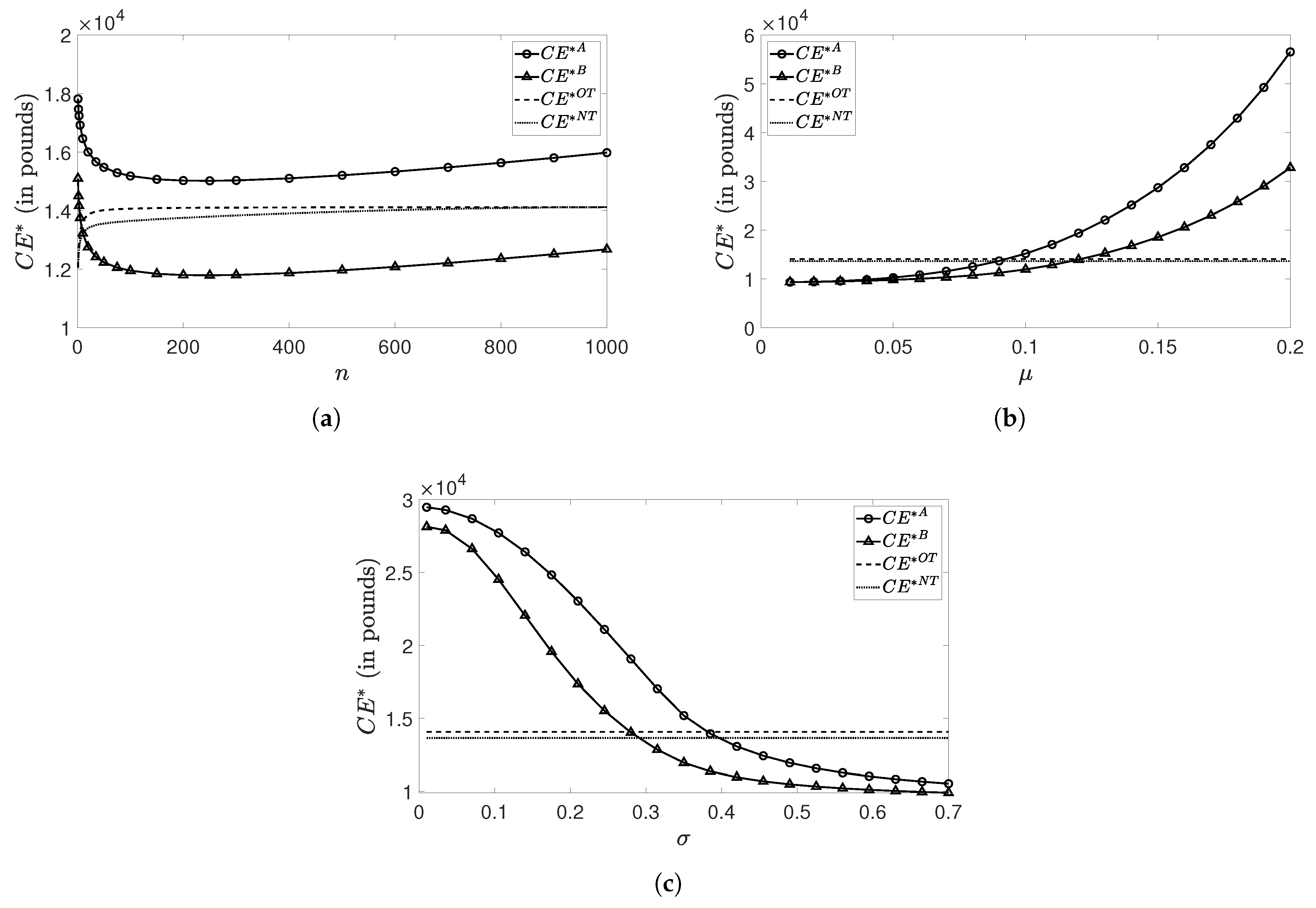
5.2.2. Numerical Results and Sensitivity Analyses

In Table 3, we show the first numerical findings, namely the ones for CE * j , that emerge from applying the baseline parameter values given in Table 1 and Table 2 (for Case B).8
Comparing the certainty equivalents reported in in Table 3 shows that the policyholder is in the best position as long as she holds the unit-linked tontine designed in Case A. When comparing only the unit-linked tontine variants, it is more beneficial for the individual if the tontine payout process does not include an additional guaranteed payment as in Case B, but rather simply complies with the entire portfolio value that arises entirely out of optimally investing in the financial market. The unit-linked tontine variant from Case B actually performs worse than the traditional tontine, where even the more practicable version, the natural traditional tontine, surpasses it by far, i.e., CE * NT CE * B . Do the previous observations also hold if certain parameter values change?
In Figure 1 and Figure 2, we show the numerical comparison findings that emerge from applying the parameter ranges given in Table 1. In particular, we present the resulting curves for CE * j if the parameters n, μ , σ , γ and ρ vary, respectively.9
Two main observations can be universally drawn from Figure 1 and Figure 2:
  • Overall, we detect in each graph that, like in Table 3, the unit-linked product from Case A provides the policyholder with a higher certainty equivalent than the one from Case B. As such, varying parameter values does not seem to affect the performance order between the two unit-linked tontine alternatives (at least not for the parameters and their ranges under consideration). Nevertheless, the performance of the tontine from Case B more and more approaches that of the one from Case A if μ decreases or if σ or γ increases;
  • There exist regions in which the unit-linked tontine variants make the individual better off than the traditional tontine variants. This is not very surprising for Case A, as is known. However, it reveals that our Case B can also outperform the traditional tontine in some parameter constellations. This emphasizes the potential attractiveness of this participating tontine, especially to customers who consider additional guarantee components important. We remark that participants preferring guarantees are typically loss averse, see e.g., Berkelaar et al. (2004); Kahneman and Tversky (1979). In particular, the unit-linked tontine performs well if n is either very low or high, if μ is high or if σ , γ or ρ is low. On the whole, we conclude that if the traditional tontine product is consulted as a basis for comparison, it is possible that the unit-linked counterpart is more successful among the customers and, thus, it seems reasonable to promote it.
As already pointed out by Chen et al. (2021) (Theorem 5.2), the impact of the pool size on the attractiveness of a tontine is not monotonically increasing. In their context, they compare tontines with annuities and the critical pool size determines the preference ordering between annuities and tontines. After the pool size reaches a certain magnitude, tontines will become, for instance, more attractive than conventional annuities. They observe that this number is rather small for a conventional tontine case. Now, in our unit-linked products, this number seems rather large, shown in Figure 1a to be larger than 200, beyond which the attractiveness of the unit-linked tontine products increases in the pool size.
In order to get a better understanding of the findings derived from Table 3 and of the above-mentioned observations based on Figure 1 and Figure 2, we show in Figure 3 the means and 0.01-/0.99-quantiles under P of the optimal total payments for Cases A and B and the traditional tontine with respect to age. For the generation of the graphs, we assume that the considered policyholder is always alive and that the parameters attain their baseline values given in Table 1 and Table 2 (for Case B).10
By comparing Case A and Case B by means of Figure 3, the effect of the guaranteed payment picked up in Case B becomes clear: In Figure 3c, we notice that the 0.01-quantile curve for Case B is almost always significantly above the one for Case A. This implies that the inclusion of the guaranteed payment prevents the policyholder in Case B from receiving a very low total payment in bad market scenarios. Yet, at the same time, the guaranteed payment also limits a possible positive development of the total payment in good market scenarios, which is, however, completely exploited by the unit-linked tontine from Case A. This is recognizable by the 0.99-quantile curves displayed in Figure 3a,b. Since the scale of the 0.99-quantiles, especially in Figure 3b, is much larger than the one of the 0.01-quantiles in Figure 3c, the dominance of Case A in good market scenarios clearly outperforms the dominance of Case B in bad market scenarios. Hence, as visible in Figure 3a,b, the mean of the total payment for Case A is consistently higher than the one for Case B. Due to the fact that the power utility function is strictly increasing, we can infer from this finding that CE * A > CE * B holds, as observed above for the given parameters. Moreover, we, particularly in Figure 3a,c, see that the curves for the traditional tontine, which is represented here by the optimal version, can be above or below the ones for the unit-linked tontine. That is why the policyholder prefers the traditional tontine to the unit-linked tontine in some instances, while in others she does not, as apparent from Figure 1 and Figure 2. The partial dominance of the traditional tontine explicitly shown in Figure 3 suffices to beat the performance of the unit-linked tontine from Case B, but not the one from Case A. This can be observed from Table 3, where all parameters also attain their baseline values.
In the following, the impacts of the parameters n, μ , σ , γ and ρ and, eventually of the varying parameters δ and g, being only related to Case B, will be discussed in detail.

Sensitivity Analyses Regarding n 

In Figure 1a, we notice right away the converse behavior of CE * A and CE * B with regard to CE * OT and CE * NT as long as the initial number n of participants in the pool ranges within relatively small values. Especially when an extremely small pool takes in a very few new participants, the policyholder’s benefit drops sharply in case of the unit-linked tontine, whereas it rises quickly for the traditional tontine. From around n = 250 on, the courses of the curves belonging to the unit-linked tontine switch to an upward movement, which becomes even steeper than the one for the traditional tontine. In summary, a purchase decision in favor of the unit-linked tontine is wise if the pool size is either very small or large.
In order to get a better understanding of the recorded observations, we let n vary again and study the resulting optimal values V 0 * A and V 0 * B ˜ for the initial investment amount in Figure 4.
We observe very similar curve shapes for V 0 * A and V 0 * B ˜ in Figure 4 compared to the ones for CE * A and CE * B in Figure 1a, namely the strong decline in n at the beginning, which quickly lessens and, from around n = 250 on, turns into an increase. Consequently, it seems that the behavior of the initial investment amount for a varying pool size causes the performance development of the unit-linked tontine described above. If we exemplarily consider the formula in (22) for V 0 * A , only the initial decrease appears plausible at first glance. However, when we recall that lower (implicit) safety loadings included in the premiums can be chosen if n grows by reducing t p ˜ x , just like we do, it is comprehensible why the decrease can be slowed down and possibly even be reversed at some point. Below, we provide more interpretations to the impact of the pool size n:
  • Unit-linked products can outperform the traditional tontines (both the natural tontine and the optimal tontine), but can also be beaten by the traditional ones. With the chosen parameters, the unit-linked tontine type A outperforms, while the unit-linked tontine type B is beaten by, the traditional ones;
  • For the given parameters, we observe that the unit-linked products with n = 1 leads to the highest utility level. It is implied that the unit-linked annuity is most favored. However, let us point out that the result depends substantially on the choice of the parameters;
  • The main message is that, depending on the design of the unit-linked tontine products including the pool size, the unit-linked tontine product can be attractive for some individuals. Among all these products, there is no dominance in terms of expected utility. The unit-linked products enriches the variety of the products.

Sensitivity Analyses Regarding  μ and  σ  

If the policyholder chooses the unit-linked tontine, we observe in Figure 1b,c that her utility enhances more and more as long as the drift rate μ of the risky asset increases and its volatility σ decreases, respectively. This is because the risky asset, in which investments are made within the framework of the unit-linked tontine, is clearly more profitable if its return grows and its risk reduces, as can be seen, for example, from a higher Sharpe ratio μ r σ , which eventually is naturally also more beneficial to the policyholder. As the certainty equivalents associated with the traditional tontine are apparently not affected by a varying μ or σ due to its payout’s independence of the financial market, there is a certain level at which the performance of the risky asset is so good that the traditional tontine is no longer preferred.

Sensitivity Analyses Regarding  γ and  ρ  

In Figure 2a, we find that CE * j declines for all j for higher values of γ , which means that each tontine variant gets less interesting for the individual when she becomes more risk-averse. This is because the risk inherent in the tontines is borne, to a great extent, by all participants in the pool, and the payments to the policyholder are, hence, uncertain to some extent. If the policyholder embraces less of this risk, i.e., she is more risk-averse and prefers more stable payments, her personal benefit is, thus, smaller. However, the curves displaying CE * A and CE * B exhibit (partly much) steeper slopes than those for CE * OT and CE * NT due to the fact that the unit-linked tontine alternatives contain more risk, namely not only the mortality risk but also the financial risk component. Therefore, if the policyholder tolerates more risk, i.e., she is less risk-averse ( γ decreases) and prefers riskier payments, the unit-linked tontine is definitely the better choice. In Figure 2b, it can be observed that when the subjective discount rate ρ grows, the personal utilities induced by buying the examined tontines constantly diminish. The only exception is the optimal traditional tontine that regains some attractiveness for higher values of ρ in consequence of the specific structure of d t * , which is explicitly given in Appendix C. Since a higher subjective discount rate means that the individual tends to consume more at earlier retirement ages, the decreases of CE * A and CE * B in ρ are explainable by the steady increases of the means of the total unit-linked tontine payments over time, as this is exemplarily illustrated in Figure 3a,b. In these two figures, we also observe that the magnitudes of the two mean curves for the unit-linked tontine variants are a lot greater compared to the traditional tontine. This gives a reason for the steeper slopes of the curves displaying CE * A and CE * B in Figure 2b.

Sensitivity Analyses Regarding  δ and g 

When considering the choice for G t as introduced in (34) and (35) for Case B, we are especially interested in the impact of the guarantee growth rate δ and the guaranteed premium fraction g on the policyholder’s tontine product preference. To analyze this, we look at the resulting curves for CE * B , CE * OT and CE * NT depicted in Figure 5, where the ranges given in Table 2 are applied.
Both graphs of Figure 5 demonstrate a similar curve progression for CE * B . In particular, the resulting certainty equivalents are negatively proportional to δ and g. However, as the payout of the traditional tontine does not depend on δ and g, neither CE * OT nor CE * NT changes. As a consequence, it is possible that the policyholder benefits more from the unit-linked tontine designed in Case B than from the traditional tontine if the guaranteed payment is low enough. On the other hand, a high guaranteed component in the unit-linked tontine may adversely affect the performance of the product due to stronger limitations on possible investment gains.

6. Conclusions

In the present article, we propose unit-linked tontine products that combine the tontine concept with the idea underlying unit-linked insurance policies, i.e., to tie payouts to the developments in the financial market. We examine a general payment structure of the product and analyze two specified payment structures. The two risk types contained in the unit-linked product are the financial risk stemming from the risky asset existing in the financial market and the mortality risk, for which we actually also incorporate the systematic part in our model. The premium required to buy the unit-linked tontine is determined in a risk-neutral pricing framework. Further, we study the optimal expected utility of an individual purchasing the unit-linked tontine by adjusting the payment structure. In our numerical comparison and sensitivity analyses, we contrast the policyholder’s benefits arising out of the two optimized unit-linked tontine variants, as well as the optimal and the natural traditional tontine. In particular, we find that there exist circumstances in which the unit-linked tontine endows the policyholder with a higher utility level than the traditional tontine, emphasizing the potential of the suggested unit-linked tontines. More precisely, under our numerical setting with power utility functions, the unit-linked tontines might be a potential choice for the policyholder when the expected return of the risky asset is high or if the volatility of the risky asset, the policyholder’s risk aversion or her subjective discount rate is low. Moreover, we observe that if its payout process is stipulated by the pure financial market portfolio value, the unit-linked tontine consistently makes the policyholder better off than in the case where it includes guaranteed payments. However, its performance approaches more and more that of the superior variant if the expected return of the risky asset decreases or if the volatility of the risky asset or the policyholder’s risk aversion increases. Furthermore, when comparing the case with guaranteed payments with the traditional tontine with no financial market component, this case can nevertheless be attractive, especially to customers who consider additional guarantee elements important. Our findings would give reason to further study this new type of product in more realistic settings that take practical aspects into account, for instance, how the provider hedges the mortality and financial market risks related to the unit-linked tontines and what the net loss of the provider is. A thorough analysis of the hedging perspective requires a more dynamic framework and will be left for future research.

Author Contributions

Conceptualization, A.C. and T.N.; Methodology, A.C., T.N. and T.S.; Software, T.S.; Writing—original draft, T.S.; Writing—review & editing, A.C., T.N. and T.S. All authors have read and agreed to the published version of the manuscript.

Funding

Thai Nguyen acknowledges the support of the Natural Sciences and Engineering Research Council of Canada [RGPIN-2021-02594].

Institutional Review Board Statement

Not applicable.

Informed Consent Statement

Not applicable.

Data Availability Statement

Not applicable.

Conflicts of Interest

The authors declare no conflict of interest.

Appendix A. Detailed Derivations

The equality in (11) holds for all t as
E Q 𝟙 ζ x > t N t = E Q t p ˜ x 1 ϵ E Q 1 N t | ζ x > t , ϵ = E Q t p ˜ x 1 ϵ E Q 1 N t 1 + 1 | ζ x > t , ϵ = E Q t p ˜ x 1 ϵ k = 0 n 1 1 k + 1 n 1 k t p ˜ x 1 ϵ k 1 t p ˜ x 1 ϵ n 1 k = E Q k = 0 n 1 n n ( n 1 ) ! ( k + 1 ) ! ( n 1 k ) ! t p ˜ x 1 ϵ k + 1 1 t p ˜ x 1 ϵ n 1 k = 1 n E Q k = 0 n 1 n k + 1 t p ˜ x 1 ϵ k + 1 1 t p ˜ x 1 ϵ n 1 k = 1 n E Q k = 1 n n k t p ˜ x 1 ϵ k 1 t p ˜ x 1 ϵ n k = 1 n E Q k = 1 n n k t p ˜ x 1 ϵ k 1 t p ˜ x 1 ϵ n k + n 0 t p ˜ x 1 ϵ 0 1 t p ˜ x 1 ϵ n n 0 t p ˜ x 1 ϵ 0 1 t p ˜ x 1 ϵ n = 1 n E Q k = 0 n n k t p ˜ x 1 ϵ k 1 t p ˜ x 1 ϵ n k 1 t p ˜ x 1 ϵ n = 1 n E Q 1 t p ˜ x 1 ϵ + t p ˜ x 1 ϵ n 1 t p ˜ x 1 ϵ n = 1 n E Q 1 1 t p ˜ x 1 ϵ n = 1 n 1 1 1 t p ˜ x 1 z n f ϵ z d z = 1 n I t .
The equality in (30) holds for all t as, with π denoting the ratio of a circle’s circumference to its diameter,
V 0 e r t ϕ d ˜ t G t ϕ d ^ t = 1 2 π e ln V 0 + r t d ˜ t 2 2 e ln G t d ^ t 2 2 = 1 2 π e ln V 0 + r t d ˜ t 2 2 e ln G t d ˜ t 2 2 d ˜ t σ π t + σ 2 π 2 t 2 = 1 2 π e d ˜ t 2 2 e ln V 0 + r t e ln G t + ln V 0 G t + r t + σ 2 2 π 2 t σ 2 2 π 2 t = 0 = 0 .

Appendix B. Proofs

Appendix B.1. Proposition 2

Proof. 
With the aid of the general pricing formula given in (13), we obtain the claim since the equality in (17) holds as
E Q Ψ t = E Q G t + α V t G t + = G t + α E Q V t G t + ,
with
E Q V t G t + = E Q V 0 e r t σ 2 2 0 t π s 2 d s + σ 0 t π s 2 d s Z G t 𝟙 Z > β t = V 0 e r t β t e σ 2 2 0 t π s 2 d s + σ 0 t π s 2 d s z ϕ ( z ) d z G t β t ϕ ( z ) d z = V 0 e r t β t σ 0 t π s 2 d s ϕ ( z ) d z G t Φ β t = V 0 e r t Φ σ 0 t π s 2 d s β t G t Φ β t = V 0 e r t Φ d ˜ t G t Φ d ^ t ,
where
β t = ln G t V 0 r t + σ 2 2 0 t π s 2 d s σ 0 t π s 2 d s .

Appendix B.2. Proposition 3

Proof. 
As the budget constraint in Problem 2 depends only on V 0 and not on π , the optimal value for V 0 is already completely determined by this constraint, so that we immediately obtain
V 0 * A = v 0 I t d t ,
which is obviously positive, so that we also stick to the condition that V 0 > 0 . Consequently, the budget constraint is entirely taken care of by V 0 * A and, thus, the determination of the optimal value of the trading strategy π can be done by simply maximizing the objective of Problem 2 with respect to π . To this end, we realize the shape of the objective as a function of π by considering the corresponding derivative:
π n V 0 * A 1 γ 1 γ 0 e ρ t κ t e 1 γ r + μ r π γ σ 2 2 π 2 t d t = n V 0 * A 1 γ 1 γ 0 e ρ t κ t e 1 γ r + μ r π γ σ 2 2 π 2 t 1 γ μ r γ σ 2 π t d t = n V 0 * A 1 γ > 0 μ r γ σ 2 π 0 e ρ t κ t e 1 γ r + μ r π γ σ 2 2 π 2 t t d t > 0 .
The identified derivative is positive (negative), i.e., the objective is strictly increasing (decreasing) in π , if
μ r γ σ 2 π > ( < ) 0 π < ( > ) μ r γ σ 2 .
Since we also need to adhere to the condition that π 0 , 1 , it is clear that, as long as μ r γ σ 2 , the optimal value for π is given by π * A = μ r γ σ 2 . Otherwise, if μ r > γ σ 2 , it is π * A = 1 . Overall, we find
π * A = μ r γ σ 2 𝟙 μ r γ σ 2 + 𝟙 μ r > γ σ 2 .

Appendix C. Review of Optimization Problem for Traditional Tontine

In the style of Problem 1, the maximization problem for the traditional tontine with the decision variable d t can be, by using (36) and replacing Ψ t by d t , formulated as follows:
max d t t 0 n 1 γ 1 γ 0 e ρ t κ t d t 1 γ d t s . t . v = P 0 = 0 e r t I t d t d t .
By applying the techniques in Chen et al. (2019), it can be shown that the optimal solution is given by
d t * = λ * e r t I t n 1 γ e ρ t κ t 1 γ ,
where the optimal Lagrange multiplier is given by
λ * = v γ 0 e r t I t 1 1 γ n 1 γ e ρ t κ t 1 γ d t γ .

Appendix D. Overview of Formulas for (Maximized) Discounted Expected Utilities

The formulas for the different (maximized) discounted expected utilities EU * j with j A , B , OT , NT that are applied for the comparison are listed in the following overview:
EU * A = n V 0 * A 1 γ 1 γ 0 e ρ t κ t e 1 γ r + μ r π * A γ σ 2 2 π * A 2 t d t , EU * B = n 1 γ 1 γ 0 e ρ t κ t G t 1 γ Φ d ¯ t * + 0 1 + α e σ π * B ˜ t y 1 1 γ ϕ y + d ¯ t * d y d t , EU * OT = n 1 γ 1 γ 0 e ρ t κ t d t * 1 γ d t , EU * NT = n 1 γ 1 γ 0 e ρ t κ t t p ˜ x M ϵ ln t p ˜ x d * 1 γ d t ,
where d ¯ t * is given as in (24), but with π replaced by π * B ˜ and V 0 replaced by V 0 * B ˜ .

Notes

1
For simplicity, we have assumed log-normal risky asset dynamics, which, as well documented, may not be very realistic. It would be interesting to look at the unit-linked tontine design problem in more general settings where the asset volatility is random when fat-tailed returns and volatility clustering are taken into account (see, e.g., Cont and Tankov 2004; Fouque et al. 2000). The continuity assumption of the stock price is relaxed in order to capture sudden and unpredictable market changes (see, e.g., Cont and Tankov 2004). Also, for such long-term investment problems, it would be more realistic to incorporate interest rate fluctuations (see, e.g., Hull and White 1990; Vasicek 1977).
2
This assumption is actually fulfilled for our specific choices of t p x and t p ˜ x in our numerical analysis, where they are given in (31) in Section 5.1.
3
Further properties of and a detailed discussion about the power utility function family can be found in, e.g., Wakker (2008).
4
In general, it is true that an optimal value for V 0 can theoretically become arbitrarily large, which would not be feasible in reality. However, due to the budget constraint, this can be prevented and, thus, choosing V 0 as a decision variable is reasonable. For example, the optimal value for V 0 in Case A given in (22) is high only when it is justified, namely if the initial wealth spent by the individual is large or if her survival probability is low, for instance.
5
It should be pointed out that G t and α can theoretically also serve as decision variables. A practicable option for G t is presented and discussed in Section 5.1.
6
We remark that a baseline γ > 1 or another type of utility function may lead to different conclusions.
7
The discounted expected utility for the natural traditional tontine diverges for too high values of γ , i.e., EU * NT goes to minus infinity if γ 1 . Consequently, we do not consult the natural traditional tontine if γ attains rather large values.
8
If the two required values π * B ˜ and V 0 * B ˜ for Case B introduced in Section 4.2 cannot be uniquely determined for the numerical outcomes in this section, this is adequately reported in the related paragraphs hereinafter.
9
Due to the divergence of the discounted expected utility for the natural traditional tontine as soon as γ gets too large, we show, in the case, where γ varies, CE * NT only as long as γ ranges within 0 , 1 . Further note that as long as we assess the sensitivity towards a parameter in any analysis in this section, all the remaining parameters attain their baseline values, if not stated otherwise.
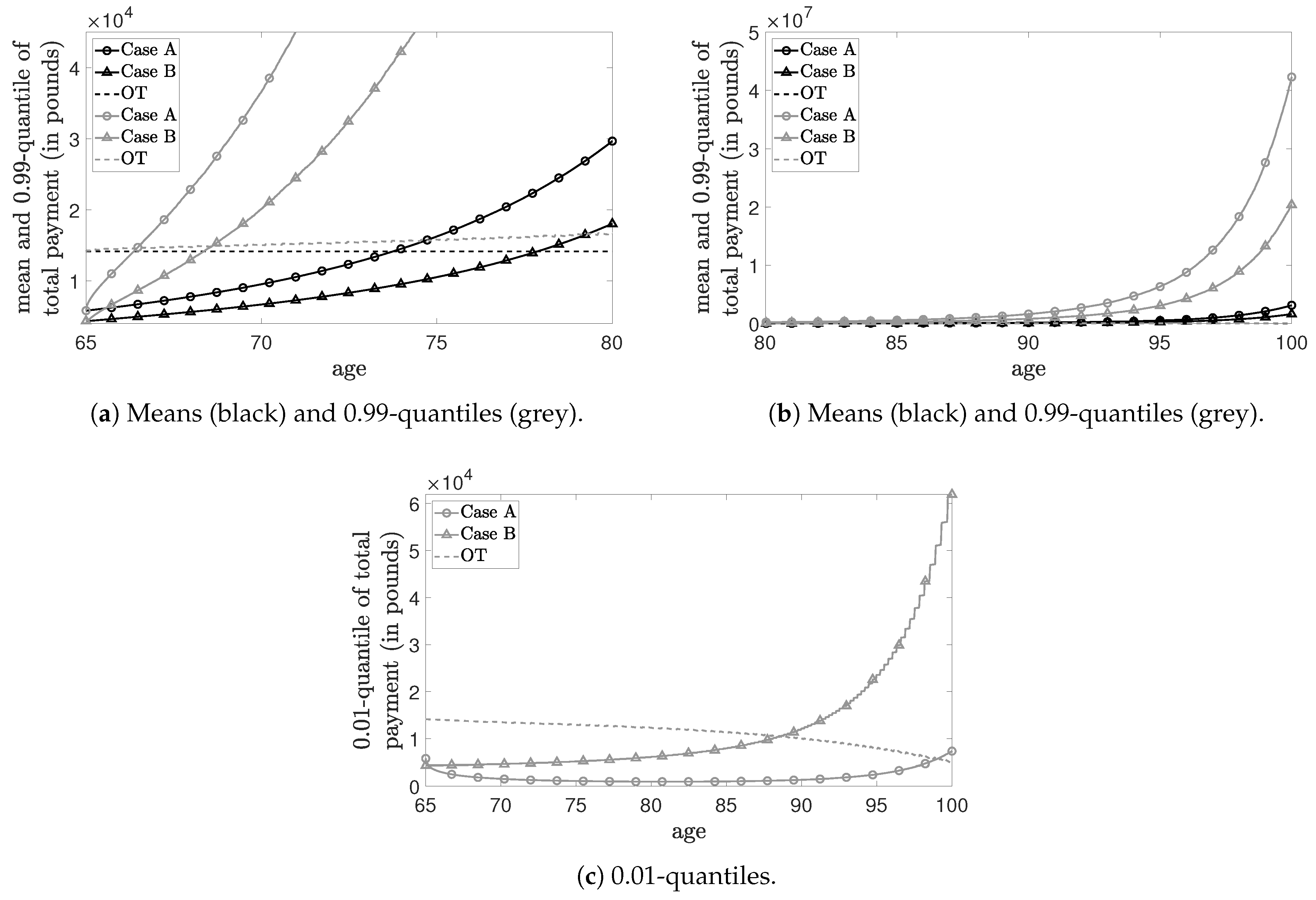
10
In detail, the applied total payments in Figure 3 are determined, for Case A, by n V t * N t , where V t * = V 0 * A e r t + μ r π * A t σ 2 2 π * A 2 t + σ π * A W t , for Case B, by n G t + α V t * G t + N t , where V t * = V 0 * B ˜ e r t + μ r π * B ˜ t σ 2 2 π * B ˜ 2 t + σ π * B ˜ W t , and, for the optimal traditional tontine, by n d t * N t . Note that the computation of all depicted quantities is done numerically, where we divide the relevant time line running from t = 0 to t = 35 by a constant discretization step size of 0.025, which means that we overall analyze 1401 points, and simulate each occurring random variable 450,000 times.

References

  1. Aase, Knut K., and Svein-Arne Persson. 1994. Pricing of Unit-Linked Life Insurance Policies. Scandinavian Actuarial Journal 1994: 26–52. [Google Scholar] [CrossRef]
  2. Bacinello, Anna Rita, Pietro Millossovich, and An Chen. 2018. The Impact of Longevity and Investment Risk on a Portfolio of Life Insurance Liabilities. European Actuarial Journal 8: 257–90. [Google Scholar] [CrossRef] [Green Version]
  3. Berkelaar, Arjan B., Roy Kouwenberg, and Thierry Post. 2004. Optimal Portfolio Choice under Loss Aversion. Review of Economics and Statistics 86: 973–87. [Google Scholar] [CrossRef]
  4. Bernhardt, Thomas, and Catherine Donnelly. 2019. Modern Tontine with Bequest: Innovation in Pooled Annuity Products. Insurance: Mathematics and Economics 86: 168–88. [Google Scholar] [CrossRef] [Green Version]
  5. Bertsekas, Dimitri P. 2014. Constrained Optimization and Lagrange Multiplier Methods. Cambridge: Academic Press. [Google Scholar]
  6. Black, Fischer, and Myron Scholes. 1973. The Pricing of Options and Corporate Liabilities. The Journal of Political Economy 81: 637–54. [Google Scholar] [CrossRef] [Green Version]
  7. Briys, Eric, and François de Varenne. 1994. Life Insurance in a Contingent Claim Framework: Pricing and Regulatory Implications. The Geneva Papers on Risk and Insurance Theory 19: 53–72. [Google Scholar] [CrossRef]
  8. Chen, An, and Manuel Rach. 2019. Options on Tontines: An Innovative Way of Combining Tontines and Annuities. Insurance: Mathematics and Economics 89: 182–92. [Google Scholar]
  9. Chen, An, Peter Hieber, and Jakob Klein. 2019. Tonuity: A Novel Individual-Oriented Retirement Plan. ASTIN Bulletin 49: 5–30. [Google Scholar] [CrossRef]
  10. Chen, An, Peter Hieber, and Manuel Rach. 2021. Optimal Retirement Products under Subjective Mortality Beliefs. Insurance: Mathematics and Economics 101: 55–69. [Google Scholar] [CrossRef]
  11. Chen, An, Linyi Qian, and Zhixin Yang. 2020. Tontines with Mixed Cohorts. Scandinavian Actuarial Journal 2021: 437–55. [Google Scholar] [CrossRef]
  12. Chen, An, Manuel Rach, and Thorsten Sehner. 2020. On the Optimal Combination of Annuities and Tontines. ASTIN Bulletin 50: 95–129. [Google Scholar] [CrossRef]
  13. Cont, Rama, and Peter Tankov. 2004. Financial Modelling with Jump Processes. CRC Mathematics Series; Chapel Hill: Chapman & Hall. [Google Scholar]
  14. Dahl, Mikkel, Martin Melchior, and Thomas Møller. 2008. On Systematic Mortality Risk and Risk-Minimization with Survivor Swaps. Scandinavian Actuarial Journal 2008: 114–46. [Google Scholar] [CrossRef]
  15. Denuit, Michel. 2019. Size-Biased Transform and Conditional Mean Risk Sharing, with Application to P2P Insurance and Tontines. ASTIN Bulletin 49: 591–617. [Google Scholar] [CrossRef]
  16. Dhaene, Jan, Alexander Kukush, Elisa Luciano, Wim Schoutens, and Ben Stassen. 2013. On the (In-)Dependence between Financial and Actuarial Risks. Insurance: Mathematics and Economics 52: 522–31. [Google Scholar] [CrossRef]
  17. Donnelly, Catherine, Montserrat Guillén, and Jens Perch Nielsen. 2014. Bringing Cost Transparency to the Life Annuity Market. Insurance: Mathematics and Economics 56: 14–27. [Google Scholar] [CrossRef]
  18. Ekern, Steinar, and Svein-Arne Persson. 1996. Exotic Unit-Linked Life Insurance Contracts. The Geneva Papers on Risk and Insurance Theory 21: 35–63. [Google Scholar] [CrossRef]
  19. Forman, Jonathan Barry, and Michael J. Sabin. 2015. Tontine Pensions. University of Pennsylvania Law Review 163: 755–831. [Google Scholar]
  20. Fouque, Jean-Pierre, George Papanicolaou, and K. Ronnie Sircar. 2000. Derivatives in Financial Markets with Stochastic Volatility. Cambridge: Cambridge School Press. [Google Scholar]
  21. Gatzert, Nadine, Carin Huber, and Hato Schmeiser. 2011. On the Valuation of Investment Guarantees in Unit-Linked Life Insurance: A Customer Perspective. The Geneva Papers on Risk and Insurance—Issues and Practice 36: 3–29. [Google Scholar] [CrossRef] [Green Version]
  22. Gemmo, Irina, Ralph Rogalla, and Jan-Hendrik Weinert. 2020. Optimal Portfolio Choice with Tontines under Systematic Longevity Risk. Annals of Actuarial Science 14: 302–15. [Google Scholar] [CrossRef]
  23. Giulietti, Corrado, Mirco Tonin, and Michael Vlassopoulos. 2020. When the Market Drives You Crazy: Stock Market Returns and Fatal Car Accidents. Journal of Health Economics 70: 102245. [Google Scholar] [CrossRef] [Green Version]
  24. Gothaer. 2021. Fondsgebundene Rentenversicherung mit Garantien. Gothaer Lebensversicherung AG. Available online: https://www.gothaer.de/privatkunden/rentenversicherung/fondsgebundene-rentenversicherung/ (accessed on 15 February 2021).
  25. Hu, Wei-Yin, and Jason S. Scott. 2007. Behavioral Obstacles in the Annuity Market. Financial Analysts Journal 63: 71–82. [Google Scholar] [CrossRef] [Green Version]
  26. Hull, John, and Alan White. 1990. Pricing Interest-Rate-Derivative Securities. The Review of Financial Studies 3: 573–92. [Google Scholar] [CrossRef]
  27. Kahneman, Daniel, and Amos Tversky. 1979. Prospect Theory: An Analysis of Decision Under Risk. Econometrica: Journal of the Econometric Society 47: 263–92. [Google Scholar] [CrossRef] [Green Version]
  28. Ledlie, M. Collin, Dermot P. Corry, Gary S. Finkelstein, A. J. Ritchie, K. Su, and D. C. E. Wilson. 2008. Variable Annuities. British Actuarial Journal 14: 327–89. [Google Scholar] [CrossRef]
  29. Leland, Hayne E. 1985. Option Pricing and Replication with Transactions Costs. The Journal of Finance 40: 1283–301. [Google Scholar] [CrossRef]
  30. Levy, Haim. 1994. Absolute and Relative Risk Aversion: An Experimental Study. Journal of Risk and Uncertainty 8: 289–307. [Google Scholar] [CrossRef]
  31. Lin, Yijia, and Samuel H. Cox. 2005. Securitization of Mortality Risks in Life Annuities. Journal of Risk and Insurance 72: 227–52. [Google Scholar] [CrossRef]
  32. Margaras, Vasilis. 2019. Demographic Trends in EU Regions. Available online: https://ec.europa.eu/futurium/en/system/files/ged/eprs-briefing-633160-demographic-trends-eu-regions-final.pdf (accessed on 15 December 2021).
  33. Merton, Robert C. 1969. Lifetime Portfolio Selection under Uncertainty: The Continuous-Time Case. The Review of Economics and Statistics 51: 247–57. [Google Scholar] [CrossRef] [Green Version]
  34. Milevsky, Moshe A. 2015. King William’s Tontine: Why the Retirement Annuity of the Future Should Resemble its Past. Cambridge: Cambridge University Press. [Google Scholar]
  35. Milevsky, Moshe A. 2020. Calibrating Gompertz in Reverse: What is Your Longevity-Risk-Adjusted Global Age? Insurance: Mathematics and Economics 92: 147–61. [Google Scholar] [CrossRef]
  36. Milevsky, Moshe A., and Thomas S. Salisbury. 2015. Optimal Retirement Income Tontines. Insurance: Mathematics and Economics 64: 91–105. [Google Scholar] [CrossRef] [Green Version]
  37. Milevsky, Moshe A., and Thomas S. Salisbury. 2016. Equitable Retirement Income Tontines: Mixing Cohorts without Discriminating. ASTIN Bulletin 46: 571–604. [Google Scholar] [CrossRef] [Green Version]
  38. Milevsky, Moshe A., Thomas S. Salisbury, Gabriela Gonzalez, and Hanna Jankowski. 2018. Annuities Versus Tontines in the 21st Century: A Canadian Case Study. Available online: https://www.soa.org/globalassets/assets/files/resources/research-report/2018/annuities-vs-tontines.pdf (accessed on 15 December 2021).
  39. Mitchell, Olivia S. 2002. Developments in Decumulation: The Role of Annuity Products in Financing Retirement. In Ageing, Financial Markets and Monetary Policy. Edited by Alan J. Auerbach and Heinz Herrmann. Berlin: Springer, chp. 3. pp. 97–125. [Google Scholar]
  40. Møller, Thomas. 1998. Risk-Minimizing Hedging Strategies for Unit-Linked Life Insurance Contracts. ASTIN Bulletin 28: 17–47. [Google Scholar] [CrossRef] [Green Version]
  41. Peijnenburg, Kim, Theo Nijman, and Bas J. M. Werker. 2016. The Annuity Puzzle Remains a Puzzle. Journal of Economic Dynamics and Control 70: 18–35. [Google Scholar] [CrossRef] [Green Version]
  42. Ramsay, Colin M., and Victor I. Oguledo. 2018. The Annuity Puzzle and an Outline of Its Solution. North American Actuarial Journal 22: 623–45. [Google Scholar] [CrossRef]
  43. Royal London. 2018. Will we Ever Summit the Pension Mountain? Royal London Policy Paper No. 21. London: Royal London Mutual Insurance Society Limited. [Google Scholar]
  44. Sabin, Michael J. 2010. Fair Tontine Annuity. Social Science Research Network. Available online: https://papers.ssrn.com/sol3/papers.cfm?abstract_id=1579932 (accessed on 26 February 2021).
  45. Schiereck, Dirk, Jochen Ruß, Rolf Tilmes, and Torsten Haupt, eds. 2020. Ruhestandsplanung—Beratungsansatz für die Zielgruppe 50plus. Wiesbaden: Springer. [Google Scholar]
  46. Schrager, David F., and Antoon A. J. Pelsser. 2004. Pricing Rate of Return Guarantees in Regular Premium Unit Linked Insurance. Insurance: Mathematics and Economics 35: 369–98. [Google Scholar] [CrossRef]
  47. Schwandt, Hannes. 2018. Wealth Shocks and Health Outcomes: Evidence from Stock Market fluctuations. American Economic Journal: Applied Economics 10: 349–77. [Google Scholar] [CrossRef] [Green Version]
  48. Sehner, Thorsten. 2021. Life and Long-Term Care Insurance: Valuation and Product Design. Ph.D. dissertation, October 2021. Ulm University of Applied Sciences, Ulm, Germany. [Google Scholar] [CrossRef]
  49. Sharpe, William Forsyth. 2017. Retirement Income Analysis with Scenario Matrices. Leland Stanford Junior University. Available online: https://web.stanford.edu/~wfsharpe/RISMAT/RIAbook.pdf (accessed on 3 March 2021).
  50. Smith, Elliot. 2020. Short-Selling Bans Sweep Europe in the Hope of Stemming Stock Market Bleeding. CNBC. Available online: https://www.cnbc.com/2020/03/17/short-selling-bans-sweep-europe-in-hope-of-stemming-stock-market-bleeding.html (accessed on 13 October 2021).
  51. Statista. 2020a. Average Risk Free Investment Rate in the United Kingdom (UK) 2015–2020. Statista GmbH. Available online: https://www.statista.com/statistics/885750/average-risk-free-rate-united-kingdom/ (accessed on 16 December 2020).
  52. Statista. 2020b. Distribution of Direct Life Insurance and Reinsurance Gross Written Premiums in the United Kingdom (UK) in 2019, by Lines of Business. Statista GmbH. Available online: https://www.statista.com/statistics/1126649/direct-and-reinsurance-life-premiums-distribution-united-kingdom-uk/ (accessed on 25 February 2021).
  53. Thomas, Philip J. 2016. Measuring Risk-Aversion: The Challenge. Measurement 79: 285–301. [Google Scholar] [CrossRef]
  54. Thomas, Philip J., Roger D. Jones, and William J. O. Boyle. 2010. The Limits to Risk Aversion: Part 1. The Point of Indiscriminate Decision. Process Safety and Environmental Protection 88: 381–95. [Google Scholar] [CrossRef]
  55. Vasicek, Oldrich. 1977. An Equilibrium Characterization of the Term Structure. Journal of Financial Economics 5: 177–88. [Google Scholar] [CrossRef]
  56. Waddington, Ian, William J. O. Boyle, and James Kearns. 2013. Computing the Limits of Risk Aversion. Process Safety and Environmental Protection 91: 92–100. [Google Scholar] [CrossRef]
  57. Wakker, Peter P. 2008. Explaining the Characteristics of the Power (CRRA) Utility Family. Health Economics 17: 1329–44. [Google Scholar] [CrossRef] [PubMed]
  58. Weinert, Jan-Hendrik, and Helmut Gründl. 2020. The Modern Tontine. European Actuarial Journal 11: 49–86. [Google Scholar] [CrossRef]
  59. Winter, Pascal, and Frédéric Planchet. 2021. Modern Tontines as a Pension Solution: A Practical Overview. Available online: https://www.researchgate.net/publication/355260987_Modern_tontines_as_a_pension_solution_a_practical_overview (accessed on 15 December 2021).
  60. Yaari, Menahem E. 1965. Uncertain Lifetime, Life Insurance, and the Theory of the Consumer. The Review of Economic Studies 32: 137–50. [Google Scholar] [CrossRef]
Figure 1. Effects of n (a), μ (b) and σ (c) on certainty equivalents.
Risks 10 00078 g001
Figure 2. Effects of γ (a) and ρ (b) on certainty equivalents.
Risks 10 00078 g002
Figure 3. Means and 0.99-quantiles at earlier retirement ages (a) and at more advanced retirement ages (b), and 0.01-quantiles (c) of optimal total payments for Cases A and B and the optimal traditional tontine (OT) depending on age, assuming that the policyholder is always alive and the parameters attain baseline values.
Risks 10 00078 g003
Figure 4. Effect of n on optimal values for the initial investment amount.
Risks 10 00078 g004
Figure 5. Effects of δ (a) and g (b) on certainty equivalents.
Risks 10 00078 g005
Table 1. Specification of relevant parameters for numerical studies.
SymbolDescriptionValueRange
nInitial number of participants100 1 , 1000
xInitial age of the participants65
μ Drift rate of the risky asset0.1 0.01 , 0.2
σ Volatility of the risky asset0.35 0 , 0.7
rRisk-free interest rate0.01
γ Measure of the policyholder’s risk aversion0.85 0 , 5 \ 1
ρ Subjective discount rate0.01 0 , 0.05
vAvailable initial wealth£260,000
g 1 First Gompertz parameter9.38
g 2 Second Gompertz parameter under P 88.85
g ˜ 2 Second Gompertz parameter under Q 94.46
η 1 Mean parameter of the truncated normal distribution 0.0035
η 2 2 Variance parameter of the truncated normal distribution 0 . 0814 2
Table 2. Specification of relevant parameters related to Case B for numerical studies.
SymbolDescriptionValueRange
α Participation rate0.9
δ Guarantee growth rate0.01 0.03 , 0.05
gGuaranteed premium fraction0.75 0 , 1
Table 3. Certainty equivalents of different tontines with baseline parameter values.
CE * A £15,180.83
CE * B £11,948.69
CE * OT £14,066.46
CE * NT £13,647.26
Publisher’s Note: MDPI stays neutral with regard to jurisdictional claims in published maps and institutional affiliations.

