Algoritmic Trading System Based on State Model for Moving Average in a Binary-Temporal Representation

Abstract

One of the most basic methods of technical analysis that is used in the practice of investment is the analysis of moving averages, usually calculated for exchange rates in a candlestick representation. The following paper proposes a new, state model, describing the process of trajectory changes in a binary-temporal representation. This kind of representation carries a significantly higher informative value than the candlestick one. The model is based on a proper definition of the moving average, proposed for a binary-temporal representation. The new model allows for exchange rate trajectory prediction in a short future window and, as a consequence, can be used to construct effective HFT systems. The article provides a concept of this kind of system and its comparison with others based on historical data for AUD/NZD exchange rate from the 2014–2020 period.

1. Introduction

Modern methods of technical analysis and course modelling for financial instruments are created mainly to support investors in decision-making (e.g., indicators) or to fully automatize the investment process (algorithmic systems, HFT (high-frequency trading) systems). High-frequency markets (e.g., FX market) allow for concluding hundreds or even thousands of short-term transactions. Realization of investment strategies for this kind of market is possible only by a total automatization of the investing process. This stems from the need of monitoring the market ceaselessly 24 h/day, while simultaneously opening multiple short-term transactions. There is also the need for psychological detachment (Aldridge 2013; Gallo 2014). Only those factors allow for reliable statistical market analysis and, as a consequence, lead to the creation of adequate investment strategies for HFT systems. Revenue in this kind of system comes from the percentage advantage of profitable transactions over the lossy ones. At the same time, the high number of transactions allows for a credible analysis of the results.

Construction of HFT systems require using advanced predictive methods (Alonso-Monsalve et al. 2020; Dempster and Leemans 2006; Evans et al. 2013). One of the most basic methods of technical analysis used in investing practice to predict changes in exchange rates is the analysis of moving averages (Kirkpatrick and Dahlquist 2010; Schlossberg 2012). However, the moving averages are usually calculated based on the course trajectory given in a candlestick representation. This kind of representation is characterized by a loss of significant information about the course and can, as a consequence, lead to assessment errors in prediction (Stasiak 2020). Therefore, a binary-temporal representation was introduced (Stasiak 2016), which results in a more precise description of the course change process. T analysis in a binary-temporal representation assigns each binary change the average value from last n changes. This, consequently, helps to define corresponding market states so that they include information about the size and duration of the change, as well as the average from previous changes. In this article, we introduce a proper definition of the moving average for a course prediction model in a binary-temporal representation. Therefore, the main goal of this article is to propose a new state model that uses the moving average mechanism and that allow for the construction of simple and financially effective HFT systems. The article is organized as follows. After this brief introduction, Section 2 introduces the description and rules for constructing the binary-temporal representation and its advantages and properties. Section 3 is devoted to state models in a binary-temporal representation. It discusses the assumptions of state modelling and presents a brief description of state models known from the literature on the subject. Section 4 introduces the methods of appointing moving averages in binary temporal representation. Assumptions of the new state model are presented, which takes into account the average from previous course changes given in a binary-temporal representation. Finally, Section 5 contains a practical implementation of applying the proposed model to the construction of an HFT system. This part of the work contains a description of the performance results for the researched system based on historical data of the AUD/NZD exchange rate. Section 6 provides a summary of conducted research.

A dedicated software written in C++ and MQL4 was created to model, build, and test the research results presented in the paper.

2. Binary-Temporal Representation

When constructing an HFT system, course modelling requires using the proper formatting of historical data. Quotations of most financial instruments change with high frequency (often few changes can happen during a single second). Many from these changes oscillate around defined values and with a very small amplitude of 1–3 pips. Those changes are in fact of a random character (noise) and do not carry any informative value, which could have been used in course modelling (Lo et al. 2000; Neely and Weller 2011). Therefore, using so-called ‘tick data’ (that is, the data regarding even the smallest change in the course, is ineffective). The amount of data and the possibility of noise affecting the change process hinders any analysis. Thus, the adequate formatting of historical data seems to be crucial. The most common data format used by both investors and researchers is the candlestick representation (Evans et al. 2013; Fischer and Krauss 2018; Rundo et al. 2019). It is surely the most popular representation of quotations, used in most economic research as well as in most presentations and market analyses on the broker platforms (MetaTrader, JForex etc.) (Gallo 2014; Burgess 2010; Schlossberg 2012).

Candlestick course, for a given timeframe, is described by four values: the opening and closing price, and the highest and lowest registered course value. The properties of the course represented in the candlestick representation are dependent on the assumed time interval and are independent of the course trajectory dynamics. This leads, in consequence, to the loss of informative value “inside” the candle. The frequency and range of the course trajectory changes are variable, dependent on the time of the day and current market situation (e.g., publishing of important data leads to an increase in change frequency, which can be lost if the candle range is too big). When using historical data in candlestick format, we often cannot distinguish how many transactions would have been concluded and if they would have ended with a loss of profit. As a result, using data in the candlestick representation can lead to faulty results of high-frequency trading market analysis, which was researched in detail (Stasiak 2020).

To filter the noise and for potential application of the model to HFT systems, a binary (Stasiak 2016) and binary-temporal (Stasiak 2018) representation was proposed. The idea for constructing those representations came from the visual point-symbolic method (De Villiers 1933), which despite its many advantages was almost totally replaced by the candlestick representation. In both binary and binary-temporal representations, the market changes are represented as a binary sequence, corresponding to the course trajectory changes. The binary-temporal representation, as compared to the binary one, also includes information about the duration of each change.

The binary representation is constructed based on a binarization algorithm. The algorithm describes the upper and lower change limit for a given course value. The limits are equal to the positive (or negative, respectively) increase of the course by a given unit (i.e., so-called discretization unit ($\delta$)). If the exchange rate drops below the lower limit, the algorithm assigns i-th change the binary value ${\epsilon }_i=0$. In case of an increase beyond the upper limit, the algorithm assigns i-th change the binary value of ${\epsilon }_i$ = 1. As a result, the course is presented as a binary sequence ${ℰ}_B$ for N observed changes:

$${ℰ}_B={\left\{{\epsilon }_i\right\}}_{i=1}^N.$$

(1)

Similarly, in case of falls in the binary-temporal representation, the binarization algorithm assigns the i-th change two values: the binary value ${\epsilon }_i=0$ and the duration of the change expressed in seconds $\Delta t_i$. Also, when an increase occurs, the algorithm assigns the value ${\epsilon }_i$ = 1 and the duration of the change $\Delta t_i$. In the next steps, the algorithm calculates the next limit values for currently registered change and notes the time passed since the end of the previous change. Eventually, we obtain a representation for the considered course trajectory in form of a sequence ${ℰ}_{BT}$ of N registered changes:

$${ℰ}_{BT}={\left\{\left({\epsilon }_i,\Delta t_i\right)\right\}}_{i=1}^N.$$

(2)

Advantages of such a course representation are registering all changes of range bigger than the discretization unit and filtration of the noise. Noting changes that are bigger than the discretization unit in the binary-temporal representation effectively eliminates the problem of losing the informative value of data, contrary to the candlestick representation. Additionally, the binary-temporal representation leads to an effective noise filtration, i.e., elimination of changes which size is smaller than the given discretization unit. The binary-temporal representation can stand as a basis to construct HFT systems. Details of such a construction are given in Section 4.

3. State Modelling in a Binary-Temporal Representation

3.1. Assumptions

The course trajectory of a given financial instrument can be seen as a change process of the market state. This process reflects the behavioral patterns of the investors. The foundation of the state modelling as well as other methods of technical analysis is the assumption about the existence of statistically more frequent patterns in exchange rate fluctuations than it would imply from the assumption of its completely random fluctuations in the rate (Peters 1996; Yao and Tan 2000; Li et al. 2019). The change patterns represent investors’ behaviors and are defined in the models as sequences of state changes. They occur as a response to the current market state. An example can be the occurrence of corrections after a certain period of increases caused by the publication of important information (e.g., about interest rates). Part of the investors assumes that the price is already overestimated and they start to sell the instrument, which leads to a fall in the price (i.e., the so-called correction). On the psychological grounds, such parameters such as risk aversion force the investors to make decisions according to some defined patterns (Oberlechner 2005). Another argument for the existence of repetitive behavioral patterns of investors is technical and fundamental analysis methods, which are popularized in numerous publications. As a result, one can assume that a large number of investors will make similar decisions and, as a consequence, will influence the course trajectory in the same way.

State modelling of the exchange rate trajectory in a binary representation consists in defining the states in such a way that the specific set of changes can be always assigned a given state. We assume that the states change at the end of change duration in the binary model. The state-space includes a limited number of states. The state model can be described by the so-called transition process graph, which shows a “picture” of the market that reflects the process of market changes. The graph presents all possible transitions between the states. Based on historical data of the considered instrument one can assign probabilities of transitions between states and next, corresponding probabilities of the future changes, which are saved in a so-called prediction table. The prediction table can, in turn, be a basis for constructing an HFT system.

3.2. Binary State Model

The first and simplest state model in the binary representation is the SMBR model (State Model in Binary Representation) (Stasiak 2016). The main idea of the model is to define the states of the market as a set of possible directions of a given number of binary changes in the course trajectory. Next, the probability of the direction of a next change is to be calculated based on the analysis of transition frequency between states. In the SMBR model, the course for N observed changes is presented as a binary sequence ${ℰ}_{\mathrm{SMBR}}$, given by (1). Therefore, we have:

$${ℰ}_B={ℰ}_{\mathrm{SMBR}}={\left\{{\epsilon }_i\right\}}_{i=1}^N.$$

(3)

SMBR model assumes, that the order of changes ${\epsilon }_i$ in its newest history (i.e., m last changes) influences the probability of the future change direction. Thus, the model uses the order and type of changes in the binary representation to analyze behavior patterns of investors, yet it does not analyze the duration of the changes.

State in SMBR model is defined as a set $S^m\left(m\in \mathbb{N}\right)$ of ensuing course changes:

$$S^m=\left\{{\epsilon }_1,{\epsilon }_2,\dots ,{\epsilon }_m\right\}.$$

(4)

Depending on the parameter m we can determinate the state space we can determinate the state space ${\Omega }_{\mathrm{SMBR}}=\left\{S_0^m,\dots ,S_k^m\right\}$ where the number of states k is described by the number of all m-element permutations with repetitions from the two-element set {0,1}:

$$k_{\mathrm{SMBR}}=2^m.$$

(5)

It is worth noting that during the observation period of N ensuing changes, the trajectory of the change process in the SMBR model would consist of N − m + 1 ensuing states.

Based on the defined states one can construct a graph of the change process, in which the states are represented by vertices and edges define the set of possible transitions between states. Each edge of the graph is assigned frequency value of the transition between given states, that are calculated based on historical data:

$$P\left(S_i\to S_j\right)=\frac{n_{S_i\to S_j}}{n_{S_i}},$$

(6)

where $n_{S_i}$ in the number of returns to the state $S_i$, and $n_{S_i\to S_j}$ is the number of transitions between $S_i$ and $S_j$. Frequencies (6) are interpreted as probability estimators for transitions between given states, and can in consequence be used in the prediction of future changes. SMBR model for a given instrument in the presented notation can be described by two parameters: $\delta$ and m (that is, the discretization unit and the number of ensuing course changes). In further considerations, it will be thus referred to by SMBR($\delta$, m). Figure 1 presents an exemplary graph of the change process for the SMBR(25,2) model.

Let us now consider the performance of the SMBR(25,2) model. The state-space consists of four states: $S_1=\left\{0,0\right\}$, $S_2=\left\{0,1\right\},S_3=\left\{1,0\right\},S_4=\left\{1,1\right\}$. Each state has two possibilities of transition to the neighboring states: first in case of the course increase and second in case of the decrease. Let us assume, that the market during the i-th change is in the state $S_1=\left\{0,0\right\}$. If an increase occurs, the next change will be equal to ${\epsilon }_{i+1}=1$ and the model will change its state to $S_2=\left\{0,1\right\}$. On the other hand, in case of a fall, the process will stay in the state $S_0=\left\{0,0\right\}$.

Based on historical data analysis, we can assess the probability distribution of transitions between particular states and then the change direction probability distributions (i.e., probabilities for increases and decreases). In the SMBR model, both of those distributions are identical. In

Table 1. Probability estimation for ups and downs of the AUD/NZD instrument in SMBR(25;3) model. Source: author.

State	Probability of Increase	Probability of Decrease	Number of Returns
{0,0,0}	0.5103	0.4897	437
{0,0,1}	0.4230	0.5770	487
{0,1,0}	0.5822	0.4178	639
{0,1,1}	0.4437	0.5563	471
{1,0,0}	0.5421	0.4579	487
{1,0,1}	0.4247	0.5753	624
{1,1,0}	0.5339	0.4661	472
{1,1,1}	0.5094	0.4906	426

we can see quotation results from the 1 January 2014–31 December 2015 time period for the AUD/NZD instrument of SMBR(25;3).

The probability distribution of the future change along with the information about a more probable change direction can stand as a recommendation for concluding transactions and can be presented in form of a prediction table (

Table 2. Prediction table for the SMBR(25,3) model of the AUD/NZD. Source: author.

State	Recommendation	Probability of Success	Number of Returns
{0,0,0}	1	0.5103	437
{0,0,1}	0	0.5770	487
{0,1,0}	1	0.5822	639
{0,1,1}	0	0.5563	471
{1,0,0}	1	0.5421	487
{1,0,1}	0	0.5753	624
{1,1,0}	1	0.5339	472
{1,1,1}	1	0.5094	426

).

Each state model allows for the construction of a prediction table of a structure presented in Table 2. Based on the prediction table one can construct an HFT system, which would automatize the investment process (Piasecki and Stasiak 2019, 2020). An example of such a system description will be given in Section 4.

SMBR model stands as a kind of base state model for binary-temporal representation of an exchange rate trajectory. In the model, only the direction of a fixed number of (m) changes is analysed. This kind of basic information hypothetically allows for a market advantage. The information is taken into account also in more advanced models. Therefore, comparing the results of the simplest model with more advanced ones allows for estimating their effectiveness. However, there is one restriction: the model does not analyze the duration of changes. Other research suggests that time has a significant predictive value.

3.3. Binary-Temporal State Model

An extension of the SMBR model that takes into consideration the duration of a change is called a state model in a binary temporal representation (SMBTR) (Stasiak 2018). The model assumes that the duration of a change has a significant influence on the probability distribution of the future change direction. This fact can be explained by psychological aspects (e.g., when the increase or decrease lasts for too long, investors start to open opposite positions). Also, the majority of investors make similar decisions based on indices that are calculated for the candlestick representation, and thus including the duration of changes (Stasiak 2020).

SMBTR model is founded on the binary-temporal representation of exchange rate trajectory changes, given in (2). A state in this model is defined similarly to the SMBR model (that is, based on previous changes (4) and additional information that can be referred from the registration of duration of changes). The parameter of registered durations for given states would have been an intuitive solution, but it would have led to the need of considering even ten thousand different states. Since the number of possible states has to be limited, the author decided to assign each i-th binary change a parameter ${\tau }_i$, describing the duration using a threshold method:

$${\tau }_i=\{\begin{array}{cccc}1,& & & \Delta t_i\ge Q_{\tau },\\ 0,& & & \Delta t_i<Q_{\tau }.\end{array}$$

(7)

In (7) we use threshold $Q_{\tau }$, which enables the distinction of the duration of particular changes. It is easy to note that $Q_{\tau }=0$ describes the elimination of time influence in the model and collapses it to the SMBR model. In the SMBTR model, the course for N observed changes is given as a sequence of binary pairs ${ℰ}_{\mathrm{SMBTR}}$:

$${ℰ}_{\mathrm{SMBTR}}={\left\{({\epsilon }_i,{\tau }_i)\right\}}_{i=1}^N$$

(8)

It is worth noting that due to the threshold method of calculating duration, ${ℰ}_{\mathrm{SMBTR}}\ne {ℰ}_{BT}$, where ${ℰ}_{BT}$ is given by (2).

The state in the SMBTR model is defined as the set $S^m$(m ∈ N) of ensuing course changes and $T^n$(n ∈ N) of ensuing durations, given in binary values:

$$S^{m,n}=\left\{S^m;T^n\right\}=\left\{{\epsilon }_1,{\epsilon }_2,\dots ,{\epsilon }_m;{\tau }_1,{\tau }_2,\dots ,{\tau }_n\right\}$$

(9)

Parameter m, similarly to the SMBR model, describes the number of historical changes, Parameters m and n describe the space the space ${\Omega }_{\mathrm{SMBTR}}=\left\{S_0^{m,n},\dots ,S_k^{m,n}\right\}$, where the number of states k is defined by the number of all (n + m)—element permutations with repetitions from the 2-element set {0,1}:

$$k_{\mathrm{SMBRT}}=2^{m+n}.$$

(10)

The state change in the SMBTR model depends only on the course change of a given discretization unit ($\delta$). Therefore, in the observation period of N ensuing course changes in the SMBTR model, the trajectory will consist of N − m + 1 ensuing states, analogously to the SMBR model.

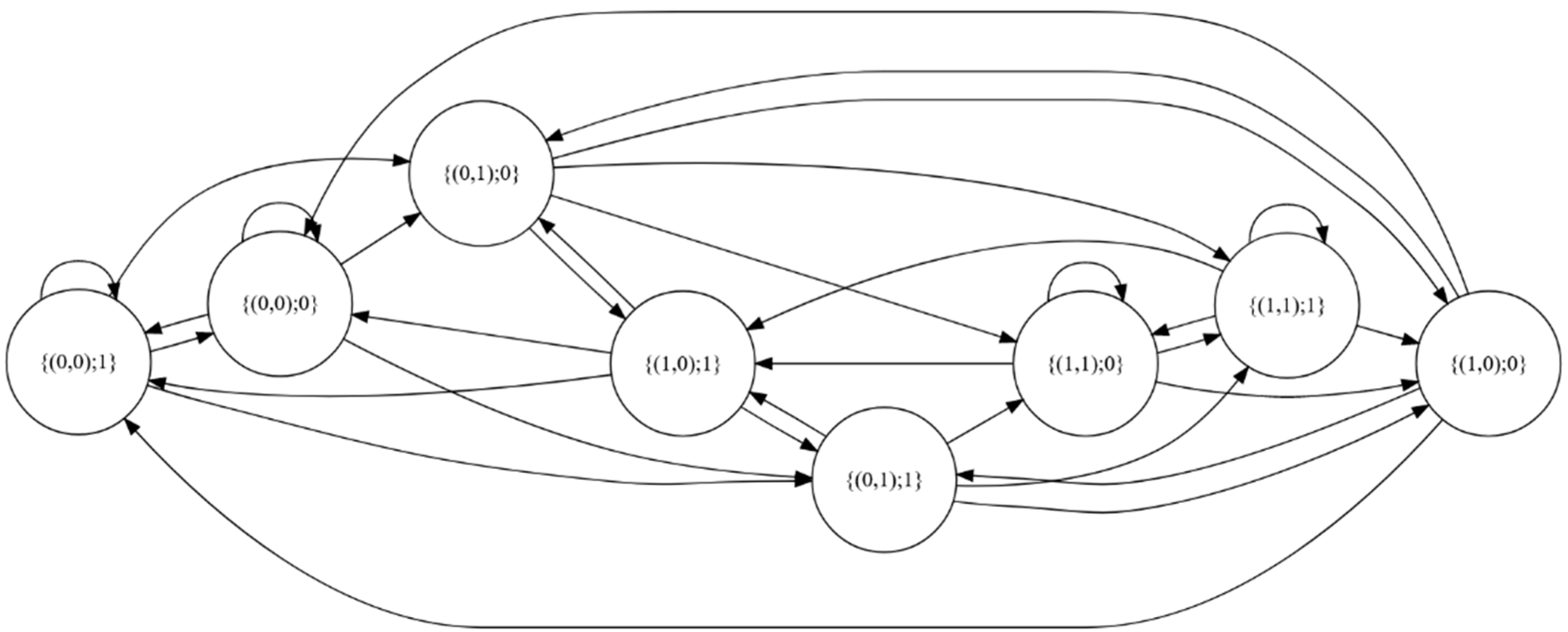
Proceeding in the same way as in the SMBR model, based on appropriately defined states, it is possible to construct a change process graph, in which states are represented by vertices, while the edges of the graph define a set of possible transitions between states. SMBTR model can be described by four parameters: m, $\delta$, $Q_{\tau }$ and n, that is the number of ensuing changes, discretization unit, the duration threshold and the number of ensuing durations, respectively. In further considerations, we will refer to it by SMBTR($\delta$, m, $n,Q_{\tau }$). Figure 2 shows an exemplary process graph for the changes in SMBTR(25,2,1,300) model.

Let us follow the performance of the SMBTR(25,2,1,300) model. We assume that the market is in the state {(0,0);1}. If an increase in the course occurs next 52 s (52 < 300), then the market will make a transition to the state {(0,1);0}. On the other hand, if a decrease occurs in next 450 s (450 > 300), then the market will stay in the {(0,0);1} state. Similarly, if next 103 sec a decrease occurs, (103 < 300), the market transitions to {(0,0);0}. Finally, if the rate increases in 512 s (512 > 300), the market reaches {(0,1);1}.

Based on the historical data analysis, we can assess the probability distribution for transitions between states, and next, the probability distribution of change direction (i.e., probability of an increase and a decrease in the quotations), for particular states. Based on the probability distributions, we can assess the probability of a future change direction.

The probability distribution calculated for transitions between states in the SMBTR model is not identical with the probability distribution of changes, similarly to the SMBR model. For each state in the SMBTR model we can distinguish four possible types of changes:

-

An increase in a time shorter than the threshold value $Q_{\tau }$;

-

An increase in a time longer than the threshold value $Q_{\tau }$;

-

A decrease in a time shorter than the threshold value $Q_{\tau }$;

-

A decrease in a time longer than the threshold value $Q_{\tau }$.

Again, similarly to the SMBR model, we can construct a prediction table, based on historical data. The prediction table can next be used to design a proper HFT system.

3.4. State Modelling with the Use of Moving Average

3.4.1. Moving Average in a Binary-Temporal Representation

The moving average is one of the basic parameters of technical analysis, used in the analysis of the course trajectory in candlestick representation. We can distinguish simple moving average (SMA), which is an arithmetic average of the closing prices from n previous candles, and a group of weighted moving averages (WMA) (Lim 2015).

Let us consider using moving averages in the analysis of course trajectory given in the binary-temporal representation. In the binary representation, it is not easy to define a simple moving average SMA. To describe an average based on only the size of a change in n periods would lose the information about the order of changes and about the times of their occurrence. Due to this observation, we introduce a so-called “binary average”, which consist in appointing an average from the binary changes expressed by the time parameter.

In the proposed method of calculating the binary average, we transform the notation of a single course change from $\epsilon ϵ\left\{0,1\right\}$ to $\phi ϵ\left\{-1,1\right\}$. In this notation, a decrease is assigned a value (−1), and the increase is assigned a 1. Therefore, for i-th change, we have:

$${\phi }_i=\{\begin{array}{r}-1\mathrm{if}{\epsilon }_i=0,\\ 1\mathrm{if}{\epsilon }_i=1.\end{array}$$

(11)

In the model, we assume that the average will be appointed based on an n-element sequence of ensuing changes. By the symbol $T_n\left(i\right)$, where $1\le i\le n$, we denote the sum of durations and first changes of the n-element sequence:

$$T_n\left(i\right)={\displaystyle \sum _{k=1}^i}\Delta t_k.$$

(12)

Each change in the considered sequence can be assigned a corresponding weight. Weight of the i-th change ${\omega }_n\left(i\right)$ is defined in the model as the ratio between the duration of first i changes $T_n\left(i\right)$, to the duration of all n analyzed changes $T_n\left(n\right)$:

$${\omega }_n\left(i\right)=\frac{T_n\left(i\right)}{T_n\left(n\right)}.$$

(13)

In the model, we assume that weight increases with the increase of the change index. This means that the newest changes (those closest to n) have the highest weight. The last, n-th change has the highest possible weight, which is 1. Now, based on the weights and their normalization to a probabilistic measure we can calculate the binary-weighted average $E\left(n\right)$:

$$E\left(n\right)={\displaystyle \sum _{k=1}^n}\frac{{\omega }_n\left(k\right)}{{\sum }_{i=1}^n{\omega }_n\left(i\right)}{\phi }_k.$$

(14)

Such construction of the average places the calculated value in the [−1, 1] interval. The inclusion of time in the determining weights for the moving average allows for obtaining better results of course modelling than the threshold time analysis in the binary-temporal model. This is proven by empiric research results performed by the Author, which is partially presented in Section 5.

3.4.2. State Model for Moving Average in a Binary-Temporal Representation

Let us now consider a model which uses information about the binary average to find the probability distribution (i.e., state model of the binary moving average (SMBMA)). The main idea of this model, as in the classic technical analysis methods, is that the current moving average influences the probability distribution of the future change of direction. The model uses binary-temporal representation given by (2).

A state in the SMBMA model is described analogously as in the SMBR as last m changes (4) and additional information that can be inferred from assigning each change an average value, calculated based on the previous sequence of n changes. However, using averages given by (15) to describe all binary states would have led to generating a large number of states which would have made the practical applications of the model rather impossible. Therefore, due to the need of limiting the general number of states, each i-th change is assigned a ${\mu }_i\left(n\right)$ parameter, describing the average from n previous changes.

$${\mu }_i\left(n\right)=\{\begin{array}{cccc}1,& & & E_i\left(n\right)\ge Q_{\mu },\\ 0,& & & -Q_{\mu }<E_i\left(n\right)<Q_{\mu },\\ -1,& & & E_i\left(n\right)\le -Q_{\mu }.\end{array}$$

(15)

where $Q_{\mu }$ is the assumed discretization threshold for the average. In the SMBMA model, the course for N observed changes is represented as a sequence of pairs ${ℰ}_{\mathrm{SMBMA}}$:

$${ℰ}_{\mathrm{SMBMA}}={\left\{({\epsilon }_i,{\mu }_i\left(n\right))\right\}}_{i=1}^N.$$

(16)

A state in the SMBMA model is defined as the set of m consecutive course changes and average from last n course changes ${\mu }_m\left(n\right)$ expressed using a threshold, calculated at the last m-th change:

$$S^m=\left\{{\epsilon }_1,{\epsilon }_2,\dots ,{\epsilon }_m,{\mu }_m\left(n\right)\right\},$$

(17)

where ${\mu }_m\left(n\right)$ is described by (16) for I = m.

Parameters m and ${\mu }_m\left(n\right)$ describe the state space ${\Omega }_{\mathrm{SMBMA}}=\left\{S_0^m,\dots ,S_k^m\right\}$, where the number of states k is defined by the multiplication of all m-element permutations with repetitions from the 2-element set {0,1} and a single element from the set {−1,0,1}:

$$k_{\mathrm{SMBMA}}=2^m\ast 3.$$

(18)

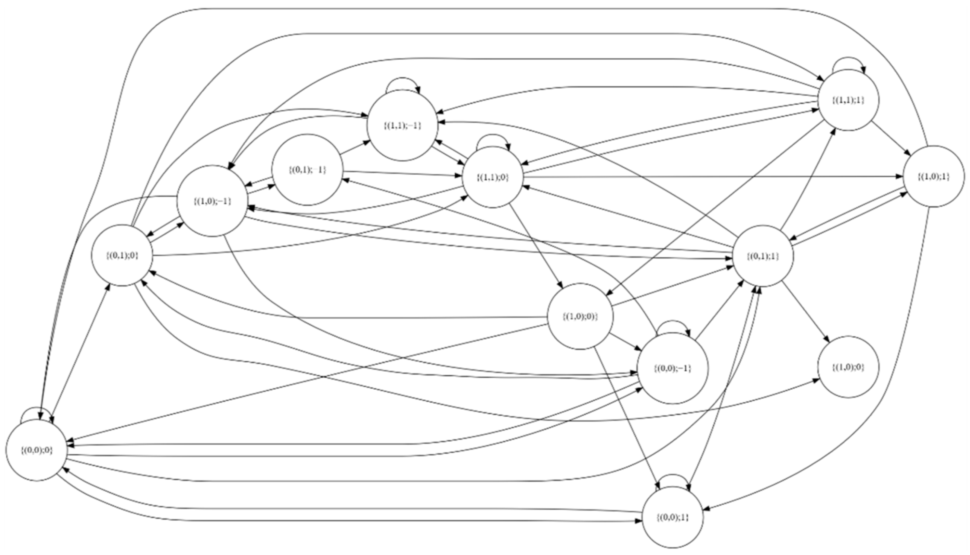
The SMBMA model is defined by four parameters: $\delta$, m, n and $Q_{\mu }$. In further considerations, it will be therefore referred to as SMBMA ($\delta$, m, n,$Q_{\mu }$). Figure 3 presents an exemplary process graph for changes in SMBMA (300,2,4,0.55) model. Since not all of the states can occur (they are dependent on the threshold, etc.) the graph shows only those states, which have occurred at least once.

In the considered model, at each state two last changes are analyzed (m = 2), as well as the binary average, described based on the four last changes (n = 4). If at any state I the average form the last four changes $E_i\left(4\right)$ is higher than $Q_i$ = 0.55, then ${\mu }_i\left(4\right)=1$. If parameter $E_i\left(4\right)$ is smaller than 0.55 and at the same time higher than −0.55, then ${\mu }_i\left(4\right)=0$. However, if the parameter $E_i\left(4\right)$ is smaller than −0.55, then ${\mu }_i\left(4\right)=-1$. Let us assume that after i-th consecutive change the market finds itself in the state {(0,0);−1}. If in the next change an increase occurs and the average will be equal to $E_i\left(4\right)$ = 0.1, then the market will make the transition to the state {(0,1);0}. On the other hand, if in the next change we have an increase but the average equals $E_i\left(4\right)$ = 0.57, then the market will go to the state {(0,1);1}.

Based on the historical data and analogously to SMBR and SMBTR models, we can calculate the probability distribution of the transitions between states. Furthermore, based on it we can create a corresponding prediction table that can be further used in the construction of an HFT system.

4. Construction of HFT Systems Based on State Models

4.1. Construction of HFT Systems

We will now consider building an HFT system that will be constructed based on the binary-temporal representation. In such kinds of systems, each binary change is assigned a transaction (Piasecki and Stasiak 2019, 2020). The transaction is opened at the beginning of the change and closet at its end. Choice of the transaction made is made based on the prediction table, depending on the state in which the market is currently at. If the transaction is concluded with a profit, the account balance $B_i$, after the i-th transaction, will increase as follows:

$$B_i=B_{i-1}+\left(\delta -r\right)\ast v,$$

(19)

where r is the spread which stands as the broker’s provision. Parameter $v$ describes the size of a pip for the instrument:

$$v=\mathrm{100,000}\ast l,$$

(20)

where l is the number of lots. If the transaction is concluded with a loss, the account balance $B_i$, after the i-th transaction, will decrease:

$$B_i=B_{i-1}-\left(\delta +r\right)\ast v.$$

(21)

According to the construction of CFD contracts, the size of profit/loss is identical in the case of both buy and sell transactions. In HFT systems transactions are opened one after another and the return rate results from the advantage of the number of profitable transactions over lossy ones. The transaction is not concluded only if the direction cannot be determined for a given state (0.5 in the prediction table).

4.2. Performance Evaluation for HFT Systems

By using the prediction table, which is determined based on historical data, it is possible to assess the usefulness of state models for the construction of HFT systems. The profit of a successful trade (19) is always smaller than the loss on the unsuccessful one (21). Thus, a system based on a given prediction table will generate profit if the following condition is met:

$$\left(\delta -r\right)v\ast P_g>\left(\delta +r\right)v\ast (1-P_g),$$

(22)

where $P_g$ is the average probability of success in a single transaction. By (23) we have:

$$P_g>\frac{\delta +r}{2\delta }.$$

(23)

Systems that do not satisfy the condition (24) cannot be further considered. If the prediction table of a given model meets the condition (24), the HFT system corresponding to this model can be verified and compared with other systems based on the so-called backtests. Backtests consist in determining the prediction table of a given system from historical data and then testing the performance of that system on historical data from a later period. As a result of a backtest, we obtain a description of dependences in balance changes over time. The results of backtests are usually presented in form of a graph of changes in the cumulative return rate $R_C\left(t\right)$.

To evaluate and compare backtests the so-called financial efficiency indicators are used. Financial efficiency is defined as the ratio of profit to the risk taken. In the case of HFT systems using CFDs, the profit is determined by the achieved return rate. Since the account balance in the case of HFT systems changes dynamically, and bankruptcy occurs only when all funds are lost, the risk is measured based on the so-called maximum drawdown $d_{max}$ (Chekhlov et al. 2005). This parameter describes the largest decrease in the cumulative return rate recorded during the backtest:

$$\begin{array}{c}\forall \\ tϵ\left(0,T\right)\wedge sϵ\left(0,t\right)\end{array}\begin{array}{c}\exists \\ d_{max}\end{array}{d}_{max}=\max \left\{R_C\left(s\right)-R_C\left(t\right)\right\}.$$

(24)

where T is the duration of the backtest. One of the most commonly used effectivity indicators is the Calmar indicator $\rho$ (Young 1991), which is defined as the ratio of the average annual rate of return $R_Y$ to the maximum decrease in the capital:

$$\rho =\frac{R_Y}{d_{max}}.$$

(25)

The higher the Calmar coefficient, the greater the profit at a given risk level. The backtest is carried out for the assumed initial balance $B_{bc}$ and the given position size $l_{bc}$. The system generates identical transaction signals, so the selection of $B_{bc}$ and $l_{bc}$ parameters does not have any influence on the indicator; the Calmar efficiency index assumes a constant value for any of their appointment.

4.3. Empirical Research of HFT Systems

Let us consider the performance of HFT systems constructed based on the binary models for the AUD/NZD course. A prediction table is required to perform a backtest, so the researched period was divided into two time periods: first, a three-year-long period of 1 January 2014–31 December 2015, in which the prediction table was determined, and then second, a three-year period between 1 January 2016–1 January 2020, where the backtest was performed. Tick data from the Ducascopy broker were used. The research assumes that the average spread offered by brokers is set to 2 pips.

We will now describe the construction of an HFT system based on the SMBR(25,3) model, where at each state three changes are analyzed. SMBR model does not analyze the duration of changes. To define the influence of the duration of changes on the effectiveness of the prediction, the SMBRT model was researched, which also takes into account three changes and the time of the last change. To determine the maximal influence of the time on the probability of success, an optimal time threshold was appointed. The best results were obtained for SMBRT(25,3,2,3610) model.

In the conducted research of the SMBMA model, the influence of the averages on the HFT system performance was taken into account. Analogously to the previous experiments, research was performed with the use of a discretization unit equal to 25, and the states were determined based on the three last course changes. Modelling results in the SMBMA model are dependent on two more parameters: the length of the sequence n for the average determination, and the appointed threshold for the discretization of the averages—$Q_{\mu }$. All sequence lengths in the 3–20 range were researched. Sequences longer than 35 did not bring any significant improvement to the prediction effectiveness. Also, all possible values for the threshold were checked, starting from 0 to 1, with the 0.05 step. The best results were obtained for the SMBMA(25,3,28,0.2) model.

Table 3. Prediction table for SMBMA(25,3,28,0.2) model of AUD/NZD, calculated for 01 January 2014–31 December 2016. Source: author.

State	Recommendation	Probability of Success	Number of Returns
{(0,0,0);−1}	0	0.54945	91
{(0,0,0);0}	1	0.51841	326
{(0,0,0);1}	1	0.65000	20
{(0,0,1);−1}	0	0.58947	190
{(0,0,1);0}	0	0.54286	210
{(0,0,1);1}	0	0.63218	87
{(0,1,0);−1}	1	0.55085	236
{(0,1,0);0}	1	0.63636	297
{(0,1,0);1}	1	0.51200	106
{(0,1,1);−1}	0	0.52764	199
{(0,1,1);0}	0	0.64557	79
{(0,1,1);1}	0	0.54922	193
{(1,0,0);−1}	1	0.50857	175
{(1,0,0);0}	1	0.56140	228
{(1,0,0);1}	1	0.55952	84
{(1,0,1);−1}	0	0.57915	259
{(1,0,1);0}	0	0.57364	129
{(1,0,1);1}	0	0.57203	236
{(1,1,0);−1}	1	0.51579	190
{(1,1,0);0}	1	0.55455	110
{(1,1,0);1}	1	0.54070	172
{(1,1,1);−1}	0	0.59375	96
{(1,1,1);0}	1	0.60000	15
{(1,1,1);1}	1	0.53651	315

shows the prediction table obtained based on the data analysis in the first research period. Analogous to the previous models, we can assess the probability of the direction of the recommended change.

Results of the modelling in the first testing period show that the introduction of the time parameter into the model allowed for an increase in the precision of calculating the probability distribution of a future change direction. Even more precise results were obtained when modelling the averages.

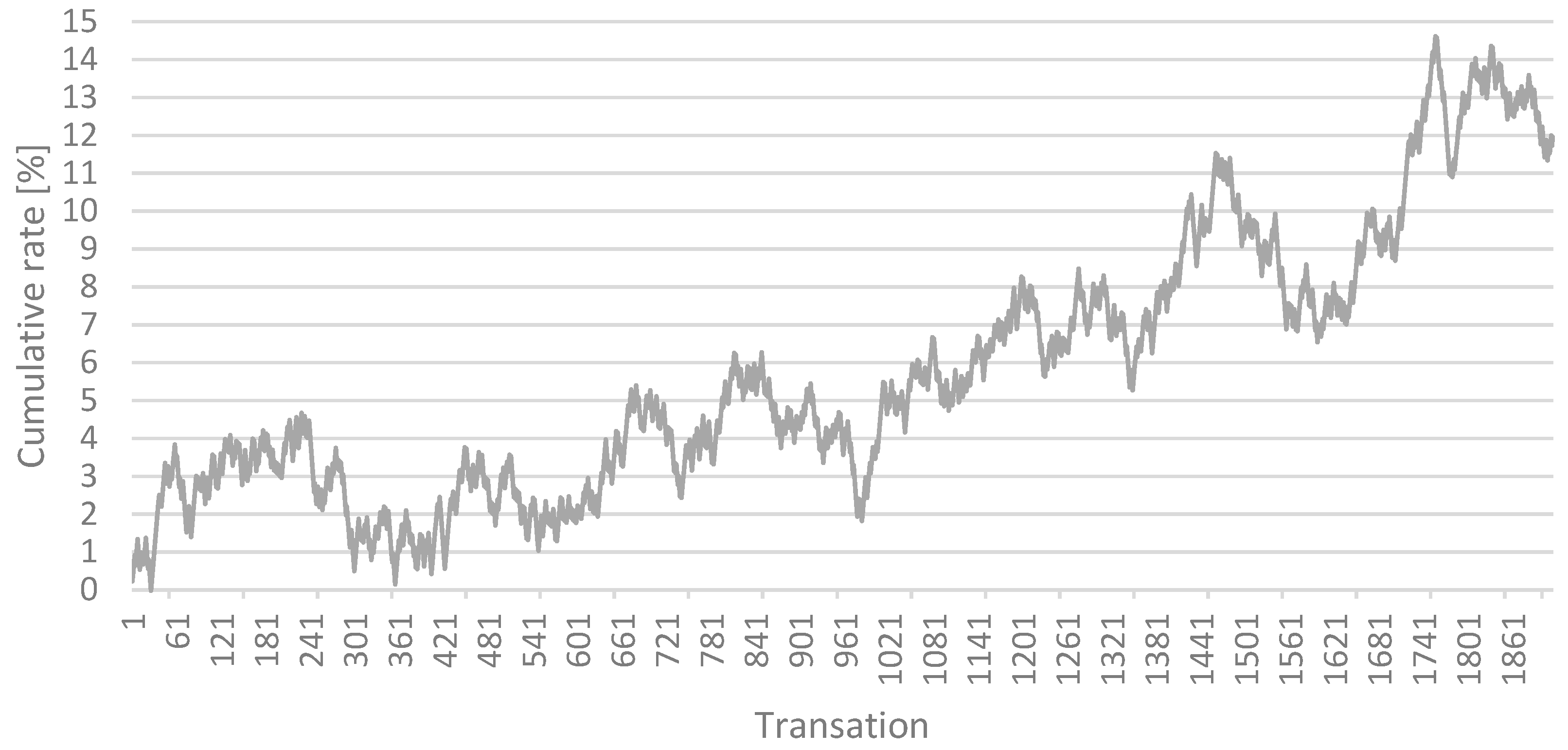
To assess the possibilities for using the obtained results in the construction of HFT systems. The initial account balance was assumed to be B₀ = 10,000 $ and the transaction size was set to l = 1 lot. Figure 4 shows the backtest results.

Based on the performed backtests, Calmar’s efficiency indicator was calculated. For the considered models it takes the following values: ρ_SMBR = 2.86; ρ_SMBRT = 3.92; ρ_SMBMA = 7.65. By analyzing the backtest, one can easily see a systematic increase of the accumulated return rate. Registered capital loses remain at a similar level; there are no drastic falls that deviate from the average. Thus, one can assume that the changes have a stable character. Beside Calmar indices, one should pay attention to the drawdown duration (Pardo 2011), which shows the maximal time after which the next capital increase is registered (here, 4.5 months).

Backtest of the systems shows similar effectiveness of prediction such as the one calculated in the predictions table. Such prediction effectiveness allows for obtaining a positive return rate according to (24).

The introduction of the duration of each change to the model (SMBRT model) led to an increase in the efficiency of the system performance. In this case, a proper HFT system can be constructed, which will allow the investor to obtain a higher systematic profit.

HFT system operating based on SMBMA model that uses a moving average from a few previous changes confirmed the efficiency of prediction stated in the prediction table. The system is characterized by the highest financial efficiency, equal to ρ_SMBMA = 7.65. Such a result means that the SMBMA model allows for achieving the highest return rate. Obtained results indicate unequivocally that the introduction of averages to the course analysis is fully justified and allows for an effective prediction of future changes and for achieving a high return rate.

5. Discussion

The research results presented in the article allow for the formulation of several conclusions of a theoretical and practical nature. In terms of theory, it can be concluded that the use of the binary-temporal representation in modelling of the exchange rate process allows for a more accurate analysis of historical data than in the case of using a candlestick representation. This is especially important for fast-changing financial instruments, since the investor’s profit or loss may be determined by unregistered changes “inside” the candle (Stasiak 2020). However, such changes are included in the binary-temporal representation, provided that the appropriate parameters for a given financial instrument are selected.

The article shows the results of an effective analysis of the exchange rate on the basis of two previously published state models in a binary-temporal representation (i.e., SMBR (Stasiak 2016) and SMBTR (Stasiak 2018)). One of the goals of this work was to answer the question whether the introduction of technical analysis methods to the course description in a binary-temporal representation will increase the predictive value of the model. To verify this, the moving average method was selected and a state model was built for the binary-temporal representation. It takes into account the average parameter in the description of the states in the exchange rate process (SMBMA model). The model introduces appropriate mean definitions, which are dependent on the assumed number of preceding changes and their duration.

The results of the research presented in the paper show that the proposed model has better predictive properties than the previous models for the binary-time representation. However, the conclusions resulting from the conducted research have a much broader context than a simple comparison of several models. It turns out that the use of technical analysis methods in state modelling (and binary-temporal representation) can significantly increase the accuracy of this modelling. The condition of success is the precise definition of the course changes process and the appropriate parameters of the technical analysis (e.g., the moving average). Those conclusions define the direction for further research, the aim of which will be to use other methods of technical analysis in modelling of exchange rates (e.g., MACD, RSI indicators). The practical result of the work presented in the article is the possibility of using the proposed models to build HFT systems. The results presented in the author’s previous works (e.g., (Piasecki and Stasiak 2019; Stasiak 2016, 2018)) indicate that the binary-temporal representation is conducive to the construction of predictive tables for such systems, and the inclusion of technical analysis methods increases their accuracy. This increased accuracy of prediction results in increased profits for the investor using those HFT systems.

6. Conclusions

The article discusses the assumptions of a new SMBMA state model for binary-temporal representation, which uses a moving average to predict market changes. During the research, assumptions for the construction of HFT systems based on appropriate state models were deduced. To verify the usefulness of researched systems in real-life investment practice and to evaluate their effectiveness, the results of empirical research on HFT systems with state models for the AUD/NZD instrument are described. The following models were compared: a binary state model, a binary-temporal state model, and a new binary average state model.

As a result of the research, it was proven that the inclusion of time in the state analysis leads to a significant improvement of the modelling results and, consequently, to higher financial efficiency in comparison with the SMBR model. The best efficiency was achieved with the SMBMA model. Thus, the proposed model allows obtaining a higher level of prediction efficiency (as compared to previous systems) and, consequently, to obtain a higher return rate in the HFT system built on its basis.

The proposed, new model allows for a next step in state modelling and construction of practical solutions that are based on its results. It is a first model that uses classic method of technical analysis that is usually applied to candlestick representation The method is modified and implemented in state modelling with a binary-temporal representation. In consequence, better results were obtained, as compared to SMBR and SMBRT models presented in previous research (which were based on relations between change parameters). The presented results indicate the direction of future research, that is modification of classic methods of technical analysis (e.g., indices) in state modelling with a binary representation.

It should be emphasized that the presented model and the method of HFT system construction presented in the article with the example of one of the very popular derivative instruments for the FX market (AUD/NZD) is universal and can be used for any financial instrument.

References

1. Aldridge, Irene. 2013. High-Frequency Trading: A Practical Guide to Algorithmic Strategies and Trading Systems. Hoboken: Wiley. [Google Scholar]
2. Alonso-Monsalve, Saúl, Andrés L. Suárez-Cetrulo, Alejandro Cervantes, and David Quintana. 2020. Convolution on Neural Networks for High-Frequency Trend Prediction of Cryptocurrency Exchange Rates Using Technical Indicators. Expert Systems with Applications 149: 113250. [Google Scholar] [CrossRef]
3. Burgess, Gareth. 2010. Trading and Investing in the Forex Market Using Chart Techniques. Chichester: John Wiley & Sons. [Google Scholar]
4. Chekhlov, Alexei, Stanislav Uryasev, and Michael Zabarankin. 2005. Drawdown measure in portfolio optimization. International Journal of Theoretical and Applied Finance 8: 13–58. [Google Scholar] [CrossRef]
5. De Villiers, Victor. 1933. The Point and Figure Method of Anticipating Stock Price Movements Complete Theory & Practice. A Reprint of the 1933 Edition including a Chart on the 1929 Crash. New York: Windsor Books. [Google Scholar]
6. Dempster, Michael, and Vasco Leemans. 2006. An automated FX trading system using adaptive reinforcement learning. Expert Systems with Applications 30: 543–52. [Google Scholar] [CrossRef]
7. Evans, Cain, Konstantinos Pappas, and Fatos Xhafa. 2013. Utilizing artificial neural networks and genetic algorithms to build an algo-trading model for intra-day foreign exchange speculation. Mathematical and Computer Modelling 58: 1249–66. [Google Scholar] [CrossRef]
8. Fischer, Thomas, and Christopher Krauss. 2018. Deep Learning with Long Short-Term Memory Networks for Financial Market Predictions. European Journal of Operational Research 270: 654–69. [Google Scholar] [CrossRef] [Green Version]
9. Gallo, Crescenzio. 2014. The Forex Market in Practice: A Computing Approach for Automated Trading Strategies. International Journal of Economics & Management Sciences 3: 169. [Google Scholar] [CrossRef] [Green Version]
10. Kirkpatrick, Charles D., and Julie R. Dahlquist. 2010. Technical Analysis: The Complete Resource for Financial Market Technicians, 2nd ed. Upper Saddle River: FT Press. [Google Scholar]
11. Li, Yang, Wanshan Zheng, and Zibin Zheng. 2019. Deep Robust Reinforcement Learning for Practical Algorithmic Trading. IEEE Access 7: 108014–22. [Google Scholar] [CrossRef]
12. Lim, Mark Andrew. 2015. The Handbook of Technical Analysis+ Test Bank: The Practitioner’s Comprehensive Guide to Technical Analysis. New York: John Wiley & Sons. [Google Scholar]
13. Lo, Andrew W., Harry Mamaysky, and Jiang Wang. 2000. Foundations of Technical Analysis: Computational Algorithms, Statistical Inference, and Empirical Implementation. The Journal of Finance 55: 1705–65. [Google Scholar] [CrossRef] [Green Version]
14. Neely, Christopher J., and Paul A. Weller. 2011. Technical Analysis in the Foreign Exchange Market. Federal Reserve Bank of St. Louis. Working Paper. Available online: https://papers.ssrn.com/sol3/papers.cfm?abstract_id=1734836 (accessed on 1 February 2022).
15. Oberlechner, Thomas. 2005. The Psychology of the Foreign Exchange Market. New York: John Wiley & Sons. [Google Scholar]
16. Pardo, Robert. 2011. The Evaluation and Optimization of Trading Strategies. New Jersey: John Wiley & Sons. [Google Scholar]
17. Peters, Edgar E. 1996. Chaos and Order in the Capital Markets: A New View of Cycles, Prices, and Market Volatility. New York: John Wiley & Sons. [Google Scholar]
18. Piasecki, Krzysztof, and Michał Dominik Stasiak. 2019. The Forex Trading System for Speculation with Constant Magnitude of Unit Return. Mathematics 7: 623. [Google Scholar] [CrossRef] [Green Version]
19. Piasecki, Krzysztof, and Michał Dominik Stasiak. 2020. Optimization Parameters of Trading System with Constant Modulus of Unit Return. Mathematics 8: 1384. [Google Scholar] [CrossRef]
20. Rundo, Francesco, Francesca Trenta, Agatino Luigi di Stallo, and Sebastiano Battiato. 2019. Grid Trading System Robot (GTSbot): A Novel Mathematical Algorithm for Trading FX Market. Applied Sciences 9: 1796. [Google Scholar] [CrossRef] [Green Version]
21. Schlossberg, Boris. 2012. Technical Analysis of the Currency Market: Classic Techniques for Profiting from Market Swings and Trader Sentiment. Hoboken: John Wiley & Sons, Inc. [Google Scholar] [CrossRef]
22. Stasiak, Michał Dominik. 2016. Modelling of currency exchange rates using a binary representation. In Proceedings of the 37th International Conference on Information Systems Architecture and Technology—ISAT 2016, Karpacz, Poland, 18–20 September 2016; Cham: Springer, 524, pp. 153–61. [Google Scholar] [CrossRef]
23. Stasiak, Michał Dominik. 2018. A study on the influence of the discretisation unit on the effectiveness of modelling currency exchange rates using the binary-temporal representation. Operations Research and Decisions 28: 57–70. [Google Scholar] [CrossRef]
24. Stasiak, Michał Dominik. 2020. Candlestick—The Main Mistake of Economy Research in High-Frequency Markets. International Journal of Financial Studies 8: 59. [Google Scholar] [CrossRef]
25. Yao, Jingtao, and Chew Lim Tan. 2000. A Case Study on Using Neural Networks to Perform Technical Forecasting of Forex. Neurocomputing 34: 79–98. [Google Scholar] [CrossRef] [Green Version]
26. Young, Terry. 1991. Calmar ratio: A smoother tool. Futures 20: 40. [Google Scholar]
Figure 1. Graph of the market change process in the SMBR(25,2) model. Source: author.
Risks 10 00069 g001
Figure 2. Graph of the change process in SMBTR(25,2,1,300) model. Source: author.
Risks 10 00069 g002
Figure 3. Graph of the change process for SMBMA (25,2,4,0.55) model of AUD/NZD. Source: author.
Risks 10 00069 g003
Figure 4. Backtest results for HFT system constructed based on SMBMA(25,3,28,0.2) model. Source: author.
Risks 10 00069 g004