Article

Impact of Climate Change on Heat Wave Risk

by
Romain Biard
1,
Christophette Blanchet-Scalliet
2,
Anne Eyraud-Loisel
3 and
Stéphane Loisel
3,*
1
Laboratoire de mathématiques de Besançon, UMR CNRS 6623, 16 route de Gray, Besançon F-25030, France
2
Université de Lyon, CNRS UMR 5208, École centrale de Lyon, Institut Camille Jordan, 36 avenue Guy de Collongue, Ecully Cedex F-69134, France
3
Université de Lyon, Université Claude Bernard Lyon 1, Institut de Science Financière et d'Assurances, 50 Avenue Tony Garnier, Lyon F-69007, France
*
Author to whom correspondence should be addressed.
Risks 2013, 1(3), 176-191; https://doi.org/10.3390/risks1030176
Submission received: 1 November 2013 / Revised: 3 December 2013 / Accepted: 5 December 2013 / Published: 12 December 2013
(This article belongs to the Special Issue Application of Stochastic Processes in Insurance)

Abstract

:
We study a new risk measure inspired from risk theory with a heat wave risk analysis motivation. We show that this risk measure and its sensitivities can be computed in practice for relevant temperature stochastic processes. This is in particular useful for measuring the potential impact of climate change on heat wave risk. Numerical illustrations are given.

1. Introduction

Climate change has now been accepted as a proven fact. The recent 5th Intergovernmental Panel on Climate Change (IPCC) Assessment Report [1], published in September, 2013, considers new evidence of climate change based on many independent scientific analyses from observations of the climate system, paleoclimate archives, theoretical studies of climate processes and simulations using climate models. The increase in the number and severity of catastrophic events may threaten the solvency of insurance companies (see [2]). However, before treating the issue of insolvency of insurance companies due to climate change, the main problem is to measure the risk and, even, to measure the impact of climate change on various risks. Current models used in insurance, to calculate premia, solvency requirements or even reinsurance policies of insurance companies are based on statistical studies using historical data. This fails to be relevant when historical data do not represent the actual evolution of indicators and, especially, with climate risk indicators, in the context of climate change. Thus, it is important to introduce new dynamic tools, as dynamic risk measures, that allow dynamic comparisons when parameters evolve. Although the risk measure developed in the present article can be used for several risk indicators, we have chosen to focus on heat wave risk. Heat waves lead to losses for insurance companies, due to the excess of mortality, business interruption or other phenomena. One of the main conclusions of the 5th IPCC report is the transient climate response, which quantifies the response of the climate system to an increasing radiative forcing on a decadal to centennial timescale. It is defined as the change in global mean surface temperature at the time when the atmospheric carbon dioxide concentration has doubled in the scenario of the concentration increasing by 1% per year. The transient climate response is likely to be in the range of 1.0 C to 2.5 C (with high confidence) and is extremely unlikely to be greater than 3 C. The global mean surface temperature change for the period 2016–2035 relative to 1986–2005 will likely be in the range of 0.3 C to 0.7 C (medium confidence). Whatever the chosen scenario is, the consequence is an increase of the global surface temperature. One question arises directly: what is the impact of this assessed global warming on the heat wave effect? In order to try to get an answer to this question, we propose a new generic risk measure adapted to climate variables (modeled as stochastic processes), in the context of climate change. In the first part, we recall the useful results of Ruin Theory and the Brownian Motion results, which we will use in the article. We study properties of this risk measure in the first part of the article. We have chosen to model temperature processes with Ornstein–Uhlenbeck (OU) processes. We derive formulas for the measure of high temperature risk. In the last part of this paper, we give a formula for the measure of the impact of an increase of temperatures on the heat wave risk measure. Numerical illustrations are given to show that the proposed risk measures and their sensitivities can be computed in practice for classical temperature processes.

2. From Ruin Theory to Climate Risk

Our main goal here is to propose a generic risk measure in the context of climate change. Given a stochastic process that describes the temporal evolution of a climate indicator, we aim at quantifying an extreme and risky behavior of this indicator, without keeping a binary view (hitting some threshold or not, for example). The indicator may be any climate process that induces a risk that may be impacted by climate change: temperature, rainfall, sea level, snow level, etc. The interest of such a risk measure is both in its dynamic and time-dependent character and its general form, which can be applied to any climate process or indicator.
Let ( X t ) be the maximum temperature process and ( Y t ) the minimum temperature process without climate change.
A heat wave corresponds to a period during which the maximum temperature is very high.
Our starting point for the construction of our risk measure is a quantity introduced in Loisel [3] related to a risk process in insurance. Let T > 0 , we thus consider first, which we call “the expected area in red” for ( X t ) , be defined as:
A X ( x ) = E 0 T | X t - x | 1 { X t > x } d t
where x represents the highest acceptable maximum temperature. However, heat waves are also characterized by the fact that the minimum temperature does not fall below some other threshold during the period. This means that A is interesting, but that we may also consider the expected area in red for ( X t ) to be restricted to high enough values of Y t :
B X , Y ( x , y ) = E 0 T | X t - x | 1 { X t > x , Y t > y } d t
Here, y represents the highest acceptable minimum temperature.

3. Modeling Temperature and Heat Wave Risk

3.1. Modeling Temperature Evolution by an Ornstein–Uhlenbeck Process

Temperature has an important seasonal component. However, the importance of the seasonality of temperature processes depends on the point of view. The literature on the modeling of temperature processes distinguishes two types of models: models for large periods of time and models for smaller period of time. In the first case, one needs to introduce some seasonality component. In the second case, the seasonality is not the major part. When studying heat wave risk, we focus on a very small period of time, from several weeks to a couple of months. In this context, the seasonality can reasonably be neglected.
The other important observed property of temperature processes is the mean-reverting property. A natural process to model seasonally adjusted temperature processes appears to be an Ornstein–Uhlenbeck process, which has been extensively used in the literature.
The authors of [4,5] were the first to present a daily simulation approach. Their approach is similar to [6], who modeled future interest rates by a continuous Ornstein–Uhlenbeck stochastic process. Later on, [8] chose to model the average historical temperature with a sine function. Brody et al. [7] introduced an Ornstein–Uhlenbeck process driven by a fractional Brownian motion, in order to take into account the long-range temporal dependencies of the temperature dynamics. Benth and Saltyte-Benth [9], presented a study of Norwegian temperature and pointed out the performance of an Ornstein–Uhlenbeck process driven by a generalized hyperbolic Levy process with time-dependent variance.
We have chosen the following model: let X t and Y t represent, respectively, the maximum and the minimum temperature process. We denote by Z t = X t - Y t the difference between minimum and maximum temperature at time t. We suppose that processes Y and Z follow Ornstein–Uhlenbeck dynamics on a probability space ( Ω , F , P ) :
d Y t = a ( b Y - Y t ) + σ Y d W t Y
d Z t = a ( b Z - Z t ) + σ Z d W t Z
with same mean-reverting speed a and where ( W Y , W Z ) is a two-dimensional Brownian motion with covariance ρ. With these conditions, the process, X t , is also an Ornstein–Uhlenbeck process, with dynamics:
d X t = a ( b X - X t ) + σ X d W t X
where:
b X = b Y + b Z
σ X = σ Y 2 + σ Z 2 + 2 ρ
W t X = σ Y σ X W t Y + σ Z σ X W t Z

3.2. Properties of the Risk Measure for OU Processes

In this section, we will study the properties of risk measures A and B defined in Section 2, in the particular case of Ornstein–Uhlenbeck processes, as introduced previously, and for a fixed time horizon, T.
A X ( x ) = E 0 T | X t - x | 1 { X t > x } d t
and
B X , Y ( x , y ) = E 0 T | X t - x | 1 { X t > x , Y t > y } d t

3.2.1. First Properties

Proposition 1. As a risk measure, A satisfies several basic properties:
  • Monotonicity: X X A X ( x ) A X ( x )
  • Translation increase of risk: k R + , A X + k ( x ) A X ( x )
  • Positive homogeneity: λ R + , A λ X ( x ) = λ A X ( x λ )
  • Homothetic property at a fixed barrier:
    Increase of risk when λ > 1 : A λ X ( x ) A X ( x )
    Decrease of risk when λ ] 0 , 1 ] : A λ X ( x ) A X ( x )
Proposition 2. B also satisfies basic properties:
  • Monotonicity: X X , Y Y B X , Y ( x , y ) B X , Y ( x , y )
  • Translation increase of risk: k , k R + , B X + k , Y + k ( x ) B X , Y ( x )
  • Positive homogeneity: λ , ν R + , B λ X , ν Y ( x , y ) = λ B X , Y ( x λ , y ν )
  • Homothetic property at a fixed barrier:
    Increase of risk when λ , ν > 1 : B λ X , ν Y ( x , y ) B X , Y ( x , y )
    Decrease of risk when λ , ν ] 0 , 1 ] : B λ X , ν Y ( x , y ) B X , Y ( x , y )
The proofs are rather direct and omitted here.
These results confirm the intuition that, in various ways, if the probability to get high values of the maximum and minimum temperature process is increased due to climate change, then the risk measures, A and B, increase, as they are penalized by this change.

3.2.2. Convex Order Property

As pointed out by one referee, one of the (claimed) consequences of climate change is not only an increase of temperature levels, but also, a tendency for more extreme weather. This can be interpreted as an increase of both the average level and variance of the temperature processes. To see the impact of a change in both levels and variability, we use the concept of increasing convex ordering.
Definition 3. Let Z 1 and Z 2 be two random variables; Z 1 i c x Z 2 (in the increasing convex order), if for all increasing convex functions ψ, such that E ( | ψ ( Z 1 ) | ) < and E ( | ψ ( Z 2 ) | ) < ,
E ( ψ ( Z 1 ) ) E ( ψ ( Z 2 ) ) .
Note that, in particular, if Z 1 i c x Z 2 , then V a r ( Z 1 ) V a r ( Z 2 ) . The following theorem shows that increasing the maximum temperature (in the convex order sense) increases risk measure A.
Theorem 4. If for all 0 t T , one has X t i c x X ˜ t (in the increasing convex order); then we have A X ( x ) A X ˜ ( x ) for all x.
Proof. Permute integral and expectation with Fubini. ☐
The following results precisely show how this translates in terms of the parameters of the Gaussian models considered in this paper.
Corollary 5. Consider two Gaussian processes, ( X t ) and ( X ˜ t ) , such that m ( t ) = E ( X t ) and V ( t ) = V a r ( X t ) (and the same with tildes). If one has for all t, m ( t ) m ˜ ( t ) and V ( t ) V ˜ ( t ) , then one has A X ( x ) A X ˜ ( x ) for all x.
Corollary 6. Consider two OU processes, ( X t ) and ( X ˜ t ) , with parameters a , b , σ and a , b ˜ , σ ˜ , such that b b ˜ and σ σ ˜ . One has A X ( x ) A X ˜ ( x ) for all x.
Proof. Let ( X t ) and ( X ˜ t ) be OU processes with parameters a , b , σ and a , b ˜ , σ ˜ . Then, their diffusion can be written as follows:
d X t = a ( b - X t ) d t + σ d W t , d X ˜ t = a ( b ˜ - X t ) d t + σ ˜ d W t
Their moments can be computed, and we have:
E ( X t ) = b ( 1 - e - a t ) + X 0 e - a t , E ( X t ˜ ) = b ˜ ( 1 - e - a t ) + X ˜ 0 e - a t
V a r ( X t ) = σ 2 1 - e - 2 a t 2 a , V a r ( X ˜ t ) = σ 2 ˜ 1 - e - 2 a t 2 a
If we have b b ˜ , then E ( X t ) E ( X t ˜ ) , and if σ σ ˜ , then V a r ( X t ) V a r ( X t ˜ ) . Then, we have X t i c x X ˜ t . ☐
Remark. If parameter b is a deterministic function, b ( t ) , then the condition becomes b ( 0 ) = b ˜ ( 0 ) and b ( s ) b ˜ ( s ) , because E ( X t ) = b ( t ) + ( X 0 - b ( 0 ) ) e - a t + 0 t b ( s ) e a ( s - t ) d s and V a r ( X t ) is unchanged.

3.2.3. Differentiability Property

Following the work of [3], it is possible to differentiate functions A X and B X , Y with respect to x and y in order to see how climate change may impact those risk measures. We begin with a sensitivity analysis of A with respect to threshold x.
Theorem 7. Function A X is differentiable with respect to x, and for all x, one has:
A X ( x ) = - E 0 T 1 { X t > x } d t
Proof. Let ϵ > 0 ; we have to compute lim ϵ 0 A X ( x ) - A X ( x + ϵ ) ϵ :
A X ( x ) - A X ( x + ϵ ) ϵ = 1 ϵ E 0 T ϵ 1 { X t > x + ϵ } d t + 1 ϵ E 0 T ( X t - x ) 1 { x X t < x + ϵ } d t
Is is obvious that the second term becomes null when ϵ tends to zero and
lim ϵ 0 1 ϵ E 0 T ϵ 1 { X t > x + ϵ } d t = E 0 T 1 { X t > x } d t .
For the new risk measure, B, we are able to carry out a similar sensitivity analysis. We start with the impact of the change of the threshold, x, that concerns the maximum temperature process.
Theorem 8. Function B X , Y is differentiable with respect to x and for all x, one has:
B X , Y ( x , y ) x = - E 0 T 1 { X t > x } 1 { Y t > y } d t
Proof. The proof is similar to the previous one. Let ϵ > 0 ; we have to compute lim ϵ 0 B X , Y ( x , y ) - B X , Y ( x + ϵ , y ) ϵ . Observing that we have:
B X , Y ( x , y ) - B X , Y ( x + ϵ , y ) ϵ = 1 ϵ E 0 T ϵ 1 { X t > x + ϵ } 1 { Y t > y } d t + 1 ϵ E 0 T ( X t - x ) 1 { x X t < x + ϵ } 1 { Y t > y } d t
we obtain the desired result after letting ϵ tend to zero. ☐
We now carry out sensitivity analysis of B with respect to threshold y, which concerns the minimum temperature process, starting with the case where the minimum temperature process, ( Y t ) , and the process, ( Z t ) (representing the difference between the minimum and maximum temperature processes), are independent.
Theorem 9. Assume that Y t and Z t are independent; then function B X , Y is differentiable with respect to y, and for all y, one has:
B X , Y ( x , y ) y = - 0 T E ( Z t - ( x - y ) ) + f Y t ( y ) d t
where f Y t is the probability density functin (pdf) of Y t (known for OU processes).
Proof.
B X , Y ( x , y ) - B X , Y ( x , y + ϵ ) ϵ = 1 ϵ E 0 T ( X t - x ) 1 { X t > x } 1 { y Y t < y + ϵ } d t = E 0 T ( Z t + Y t - x ) 1 { Z t + Y t > y } 1 { y Y t < y + ϵ } ϵ d t
Then, we obtain that:
E 0 T ( Z t + y - x ) + 1 { y Y t < y + ϵ } ϵ d t B T ( x , y ) - B T ( x , y + ϵ ) ϵ
E 0 T ( Z t + y - x + ϵ ) + 1 { y Y t < y + ϵ } ϵ d t
With Fubini and using the independence between Y and Z, we obtain:
0 T E ( Z t + y - x ) + E 1 { y Y t < y + ϵ } ϵ d t B X , Y ( x , y ) - B X , Y ( x , y + ϵ ) ϵ 0 T E ( Z t + y - x + ϵ ) + E 1 { y Y t < y + ϵ } ϵ d t
Then, applying Lebesgue’s theorem, we obtain the result. ☐
Theorem 10. The function, B X , Y , is differentiable with respect to y, and for all y, one has:
B X , Y ( x , y ) y = - 0 T E ( Z t - ( x - y ) ) + f Y t | Z t ( y ) d t
where f Y t | Z t is the pdf of Y t | Z t .
Proof. This is similar as the previous case. Notice that one may write:
0 T E ( Z t + y - x ) + 1 { y Y t < y + ϵ } ϵ d t B X , Y ( x , y ) - B X , Y ( x , y + ϵ ) ϵ 0 T E ( Z t + y - x + ϵ ) + 1 { y Y t < y + ϵ } ϵ d t
Note that we need:
( Z t - ( x - y ) ) + max b f Y t | Z t ( y ) = ( Z t - ( x - y ) ) + e - 1 + ρ σ Y t 2 ( σ Z t 2 - 1 ) 2 ρ σ Y t 2 σ Z t 2 ( Z t - E ( Z t ) ) 2
to be integrable on [ 0 , T ] × Ω . ☐
A similar analysis may be conducted with non-constant coefficients, leading to more sophisticated temperature processes.

4. Numerical Studies

In this section, we aim at computing Equations (6) and (8) numerically in order to get the value of A-measure Equation (1) and B-measure Equation (2) by integration. To avoid confusion, we omit writing the dependence on X and Y. We also study the impact of moving up the temperature process (translation of sample paths), which means either moving the barrier down for A or moving both barriers down for B. Due to adaptation or mitigation effects, it might be interesting to move down the two barriers of B by different amounts. The results are below.

4.1. A-Measure

First of all, let us remark that:
A ( x ) = - E 0 T 1 { X t > x } d t
can be rewritten as:
A ( x ) = - 0 T P ( X t > x ) d t .
Since X t is Gaussian for all t 0 , the numerical computation can be easily done.
Now, since lim x A ( x ) = 0 , we have, for all x > 0 :
A ( x ) = - x + A ( u ) d u .
This procedure to get A-measure has be done for two different processes.
  • The first one (Model 1) is the classical OU-process Equation (5):
    d X t = a ( b X - X t ) + σ X d B t
  • The second one (Model 2) is the OU-process, ( X ( t ) ) t 0 , proposed by Benth and Šaltytė Benth [10], which follows:
    d X ( t ) = d s ( t ) - κ ( X ( t ) - s ( t ) ) d t + σ ( t ) d B ( t )
    so:
    X ( t ) = s ( t ) + ( X ( 0 ) - s ( 0 ) ) e - κ t + 0 t σ ( u ) e - κ ( t - u ) d B ( u )
    where:
    • s ( t ) = α + β t + i = 1 I 1 a i sin ( 2 i π ( t - f i ) / 365 ) + j = 1 J 1 b j cos ( 2 j π ( t - g j ) / 365 ) is a deterministic function modeling the trend and seasonality of temperature;
    • σ ( t ) = γ + i = 1 I 2 c i sin ( 2 i π t / 365 ) + j = 1 J 2 d j cos ( 2 j π t / 365 ) 1 / 2 is a deterministic function describing the daily volatility of temperature variations.
In their paper, Benth and Šaltytė Benth [10] have fitted the parameters of this model on daily average temperature observations (measured in degrees Celsius) for Stockholm, Sweden, in the period January 1, 1961 until May 25, 2006. The parameters of this model are summed up in Table 1.
Although the process Equation (11) does not model daily maximum temperatures or minimum temperatures, but daily average temperatures, we have chosen to apply our A-measure on it as the first study.
Table 1. Fitted parameters in the model of Benth and Šaltytė Benth [10], for daily average temperature observations (measured in degrees Celsius) for Stockholm, Sweden, in the period January 1, 1961 until May 25, 2006.
καβ I 1 J 1 b 1 g 1 γ I 2
0 . 1994 6 . 38 0 . 0001 01 10 . 44 - 154 . 76 6 . 12 4
c 1 c 2 c 3 c 4 J 2 d 1 d 2 d 3 d 4
1 . 04 - 0 . 21 0 . 66 - 0 . 02 42 1 . 19 0 . 27 - 0 . 08
In order to compare the two models and since we are mostly interested in the summer period, we choose a = κ = 0 . 1994 , b X = s ( 1 / 2 ) = - 2 . 933048 and σ X 2 = σ 2 ( 1 / 2 ) = 9 . 521374 .
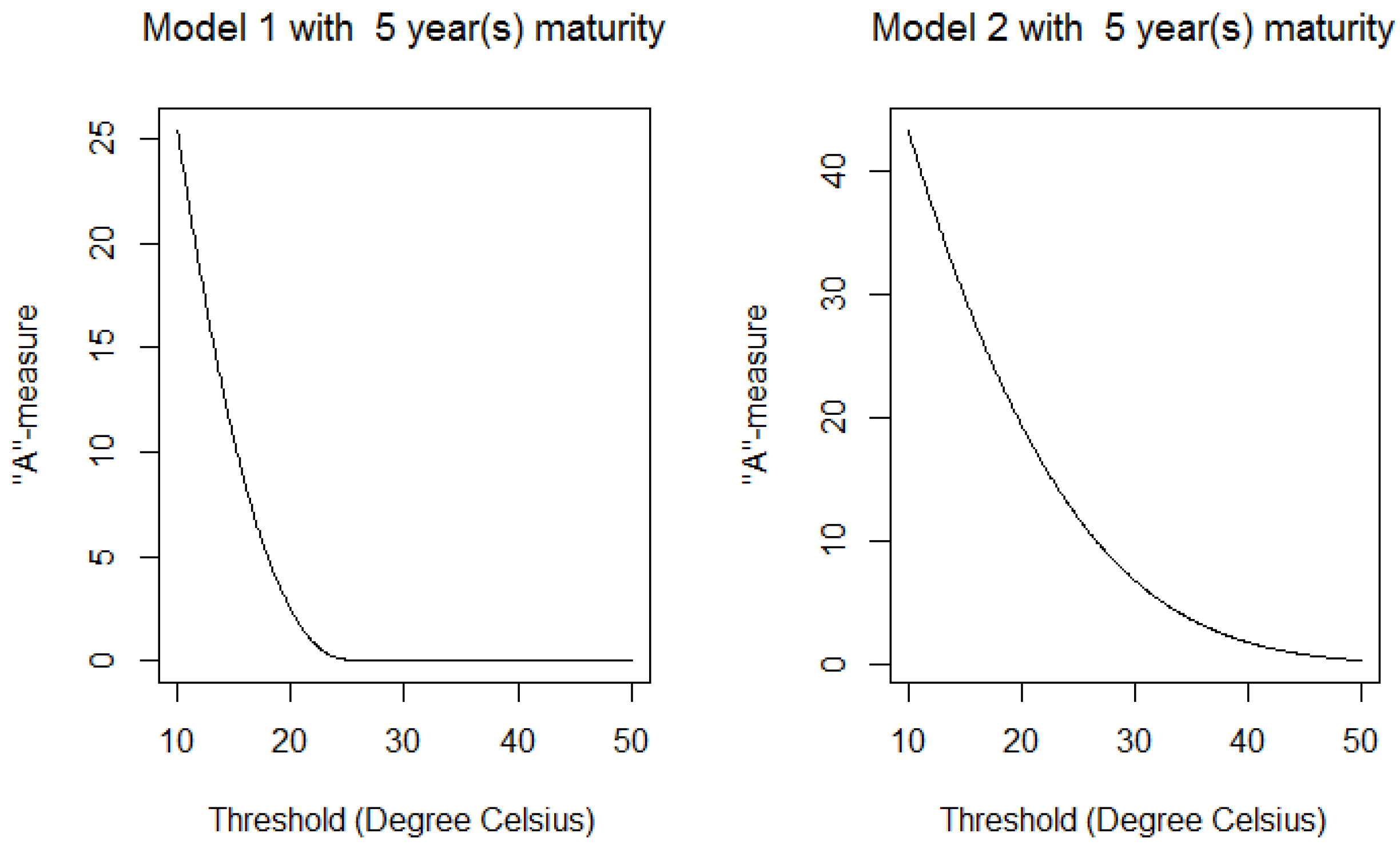
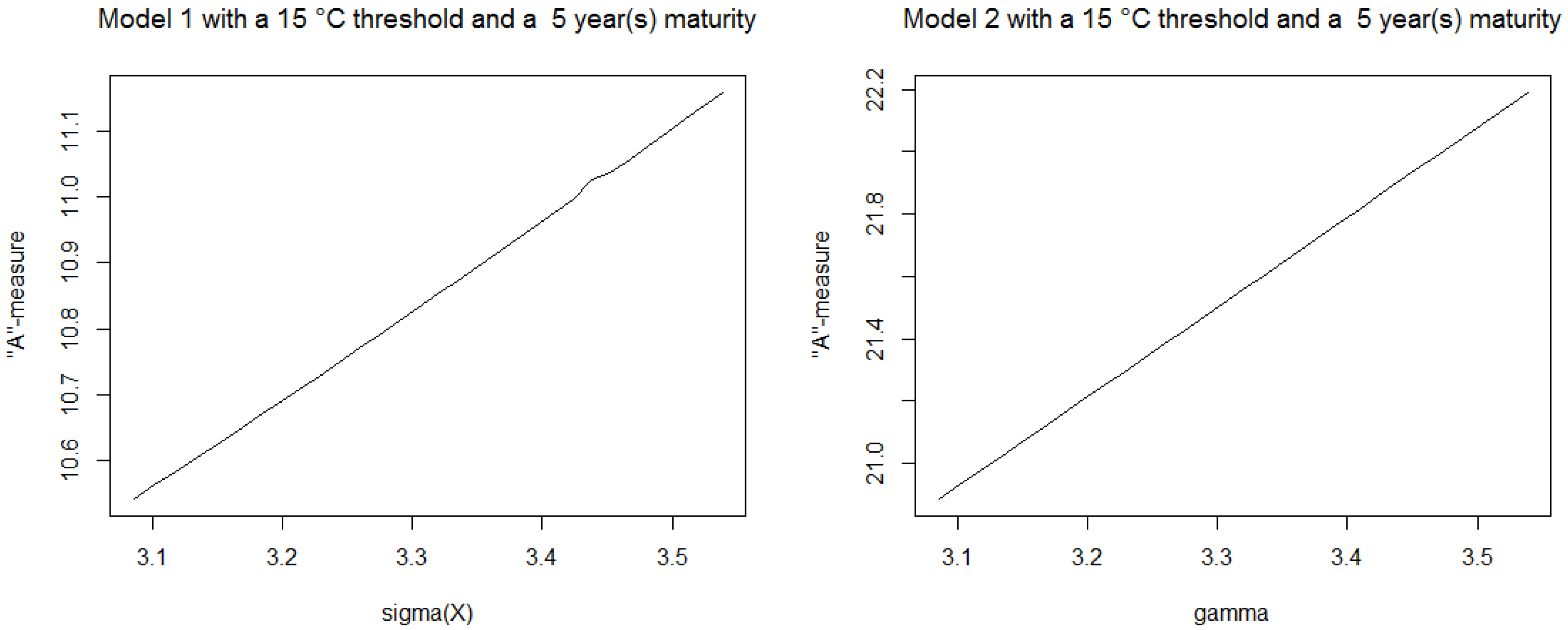
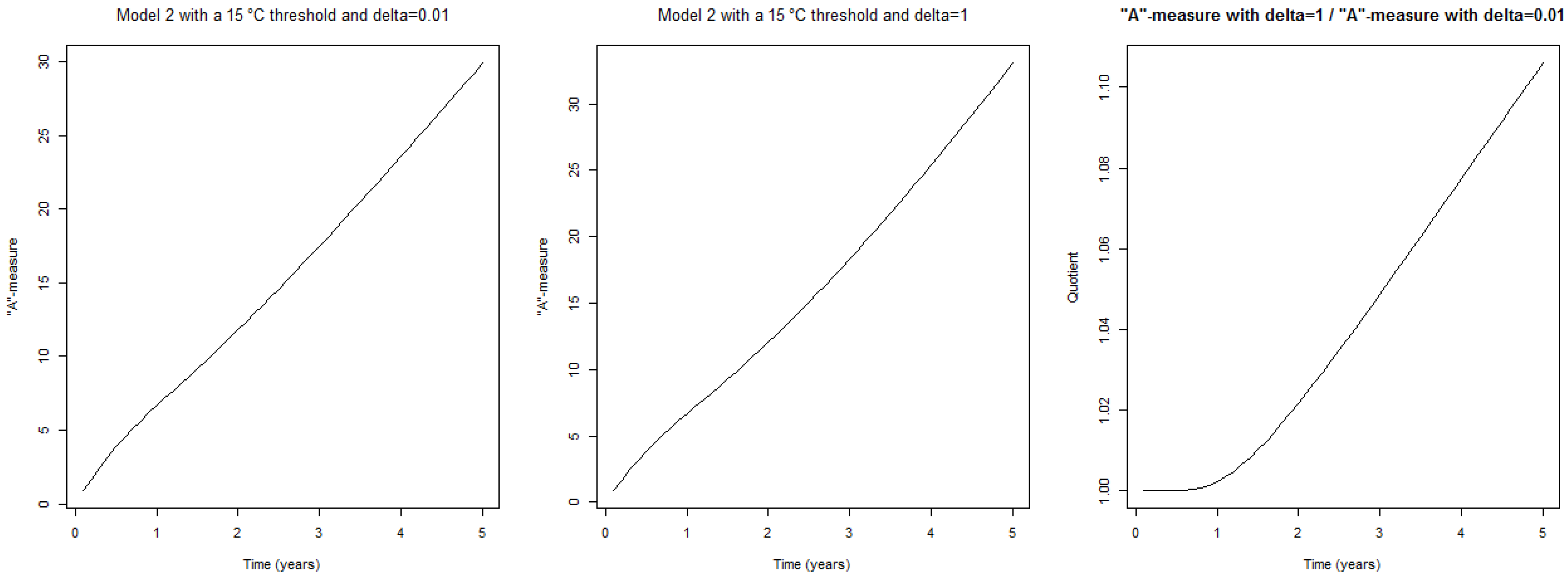
Remark. Let us first remark that in Figure 1, Models 1 and 2 are quite similar for short maturity times (six months, one year and twp years), but more different for long maturity time (five years). This is as expected, since in Model 1, trend and seasonality are not taken into account, as opposed to Model 2. To model long-term temperature, Model 2 seems more appropriate. In Figure 1, the shape of the curve is more different for a high threshold between the two models. It seems to be that Model 2 better captures global warming, so when time is large, the A-measure is higher, since the process is higher. This fact is strengthened by Figure 2. Until approximately two years, values of A-measure are quite similar. After that, it is not the case anymore. In Figure 2, the shapes of the curves are totally different. For Model 1, A-measure is like x 1 - e - x with respect to the maturity time, and for Model 2, it seems to be more linear. In Figure 3, A-measure is a function of the volatility. Regarding Model 1, A-measure is plotted as a function of σ X . Regarding Model 2, A-measure is plotted as a function of γ. For both models, A-measure seems to increase linearly with the volatility. We end this numerical study of A-measure with Figure 4. We observe here the impact of a linear time increase of σ 2 ( t ) in Model 2. We now have:
σ ( t ) = γ + δ t + i = 1 I 2 c i sin ( 2 i π t / 365 ) + j = 1 J 2 d j cos ( 2 j π t / 365 ) 1 / 2
in Equation (11). Two cases are plotted: δ = 0 . 01 and δ = 1 ; and A-measure is a function of the time maturity. We have also plotted the quotient of the two quantities. In both cases, the shape of the curve is the same as in Figure 2 with no trend in the volatility. A positive trend in the volatility increases A-measure.
Figure 1. A-measure for both Model 1 Equation (10) and Model 2 Equation (11) with initial temperature equal to 24 C and maturity time equal to six months (at the top-left corner), one year (at the top-right corner), two years (at the bottom-left corner) and five years (at the bottom-right corner). A-measure is plotted as a function of threshold (from 10 C to 50 C).
Risks 01 00176 g001aRisks 01 00176 g001b
Figure 2. A-measure for both Model 1 Equation (10) and Model 2 Equation (11) with initial temperature equal to 24 C and threshold equal to 15 C. A-measure is plotted as a function of the time of maturity (from zero to five years).
Risks 01 00176 g002

4.2. B-Measure

For the B-measure, the procedure is quite similar. Let us first remark that for U N ( m , σ 2 ) , ( u R ) :
E ( U - u ) + = σ 2 π e - ( u - m ) 2 2 σ 2 - ( u - m ) ϕ ( m - u σ ) .
With this remark, Equation (8) can be easily numerically obtained. Now, to get B ( x , y ) , we notice that lim y + B ( x , y ) = 0 , so:
B ( x , y ) = - y + B ( x , u ) y d u .
Figure 3. A-measure for both Model 1 Equation (10) and Model 2 Equation (11) with initial temperature equal to 24 C, threshold equal to 15 C and time of maturity equal to five years. A-measure is plotted as a function σ X for Model 1 Equation (10) (from 9 . 521374 to 9 . 521374 + 3 ) and γ for Model 1 Equation (10) (from 9 . 521374 to 9 . 521374 + 3 ).
Risks 01 00176 g003
Figure 4. A-measure for Model 2 Equation (11) with new volatility Equation (12) with δ = 0 . 01 and δ = 1 , initial temperature equal to 24 C and threshold equal to 15 C. A-measure is plotted as a function of time of maturity (from zero to five years). The right-hand side graph is the quotient between the two others quantities.
Risks 01 00176 g004
Let us briefly recall the model we used here described in Subsection 3.1. We study a model with two independent OU-processes. One, ( Y t ) t 0 , models the minimum temperature, and the other, ( Z t ) t 0 , models the difference between the maximum temperature, ( X t ) t 0 , and the minimum temperature, ( Y t ) t 0 . The processes are given by Equations (3)–(5).
For the process, Y, we choose the same parameters as Model 1 Equation (10) in Subsection 4.1, that is to say that a = 0 . 1994 , b Y = - 2 . 933048 and σ Y 2 = 9 . 521374 . For the process, Z, a-parameter is the same, and we choose b Z = 5 and σ 5 2 = 9 .
Figure 5. B-measure for the Model described in Subsection (3.1) with initial temperature equal to 15 C for the minimal temperature and 22 C for maximum temperature and maturity time equal to six months (at the top-left corner), one year (at the top-right corner), two years (at the bottom-left corner) and five years (at the bottom-right corner). B-measure is plotted as a function of both the threshold of the minimum temperature (from 5 C to 20 C) and the maximum temperature (from 5 C to 20 C).
Risks 01 00176 g005
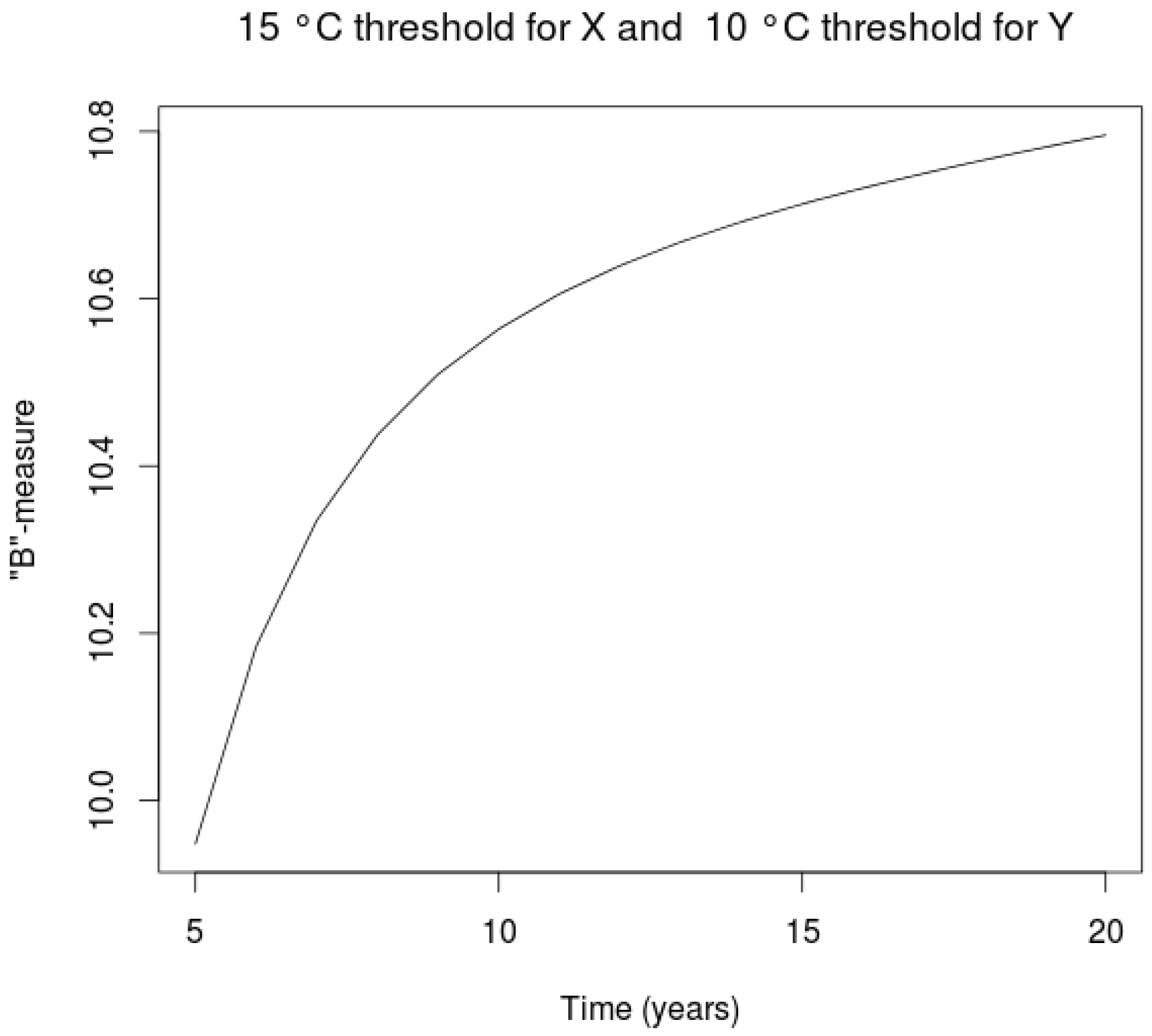
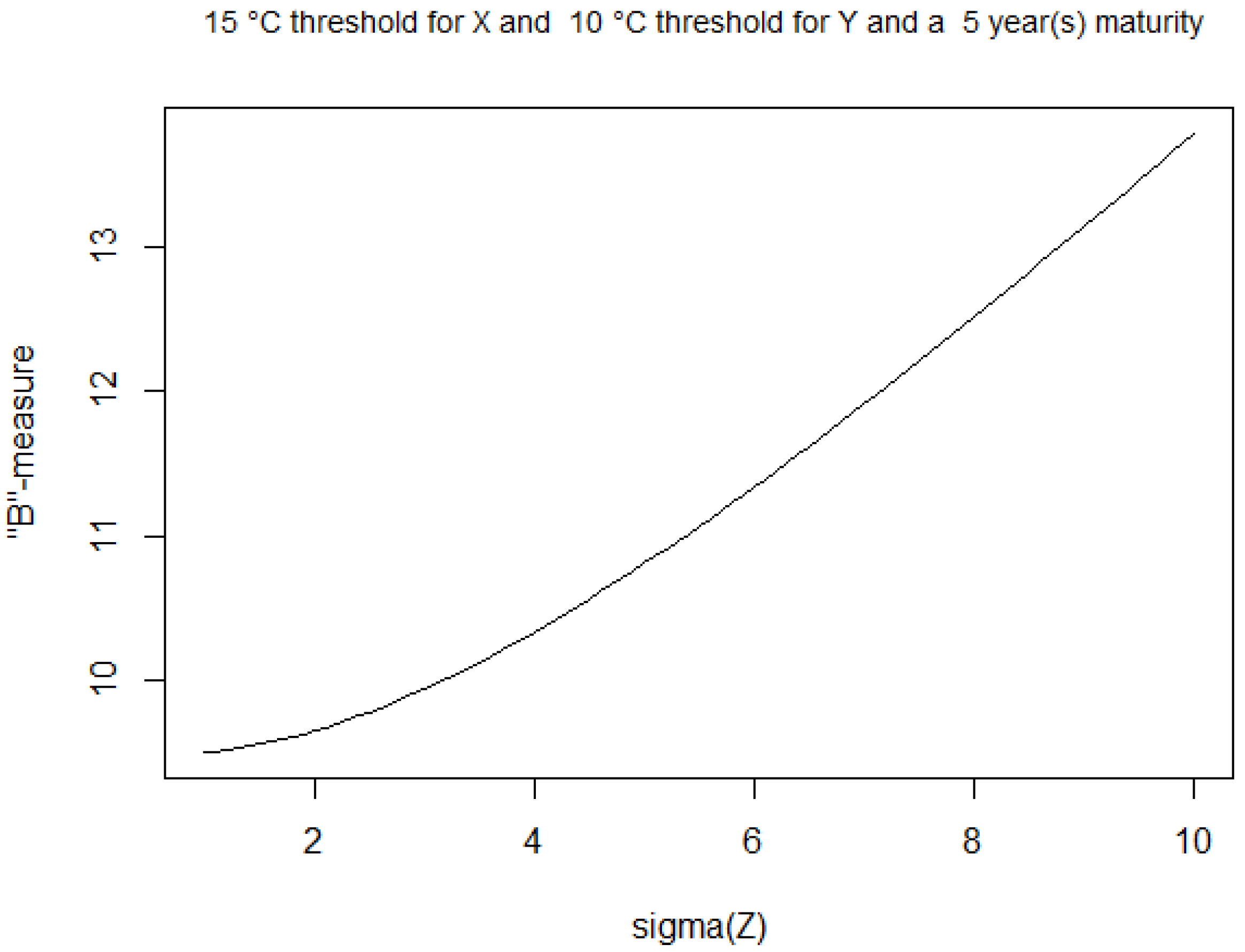
Remark. In Figure 5, the interesting parts of the plots are the parts where the threshold of maximum temperature X is higher than the threshold of minimum temperature Y, as expected in real life. In Figure 5, surfaces are more curved when the maturity time is small. In Figure 6, we retrieve the same shape as in Figure 2. A-measure and B-measure seem to behave in the same way with respect to the maturity time for classical OU-processes. In Figure 7 and Figure 8, we study the effect of volatilities on B-measure. First, the effect of the change of the volatility of one process (minimum temperature ( Y t ) t 0 ; Figure 7) is observed. Second, the effect of the volatility of the difference process ( ( Z t ) t 0 ; Figure 8) is observed, as well. Theses changes of volatilities have the same effect on B-measure: a convex increase.
Figure 6. B-measure for the model described in Subsection 3.1 with initial temperature equal to 15 C for the minimal temperature, 22 C for the maximum temperature and threshold equal to 10 C for the minimum temperature and 15 C for the maximum temperature. B-measure is plotted as a function of the time of maturity (from five to 20 years).
Risks 01 00176 g006
Figure 7. B-measure for the model described in Subsection 3.1 with initial temperature equal to 15 C for the minimal temperature, 22 C for the maximum temperature and threshold equal to 10 C for the minimum temperature and 15 C for the maximum temperature. The time of maturity is equal to five years. B-measure is plotted as a function of σ Y (from one to 10).
Risks 01 00176 g007
Figure 8. B-measure for the model described in Subsection 3.1 with initial temperature equal to 15 C for the minimal temperature, 22 C for the maximum temperature and threshold equal to 10 C for the minimum temperature and 15 C for the maximum temperature. The time of maturity is equal to five years. B-measure is plotted as a function of σ Z (from one to 10).
Risks 01 00176 g008

5. Remarks and Extensions

This paper is the first step to tackling the problem of measuring climate risk. We have shown that risk measures A X and B X , Y have desirable properties and may be computed in practice for relevant temperature processes and that it is possible to carry out a sensitivity analysis of those indicators to study the impact of climate change. Our approach can be largely improved, and we give some proposals here.
  • A heat wave is defined by “Météo France” as a sequence of at least three consecutive days for which the highest temperature is larger than a high-level temperature and the lowest temperature is greater than a low-level temperature (both high- and the low-level temperatures depend on the geographical zone). For n 1 , define X ¯ ( n ) = sup n - 1 t n X t and X ̲ ( n ) = inf n - 1 t n X t . In this context, it could be also interesting to look at the expectation of the quantity, like:
    n = 1 N X ¯ ( n ) > r u , X ̲ ( n ) > r d f X ¯ ( n ) - r u , X ̲ ( n ) - r d
    with f a function to be defined.
  • For some events, the extreme behavior of several quantities at the same time can breed a major risk. For example, both high wind and high temperature have to be taken into account in wildfire risk. Therefore, we could imagine quantities, like, for two processes, ( X t ) t 0 and ( Y t ) t 0 , and relative constants, r X and r Y :
    0 T X t > ( < ) r X , Y t > ( < ) r Y f | X t - r X | , | Y t - r Y | d t
    where f is a function to be defined.

Acknowledgments

This work has been supported by the Chair “Actuariat Responsable: gestion des risques naturels et changements climatiques”, funded by Generali since 2010.

Conflicts of Interest

The authors declare no conflict of interest.

References

  1. IPCC. Stockholm, Sweden, 23–26 September 2013; Geneva, Switzerland: Intergovernmental Panel on Climate Change, 2013.
  2. M.L. Weitzman. “On modeling and interpreting the economics of catastrophic climate change.” Rev. Econ. Stat. 91 (2009): 1–19. [Google Scholar] [CrossRef]
  3. S. Loisel. “Differentiation of some functionals of risk processes, and optimal reserve allocation.” J. Appl. Probab. 42 (2005): 379–392. [Google Scholar] [CrossRef]
  4. R. Dishel. “A Weather Risk Management Choice: Hedging with Degree-Day Derivatives.” In Insurance and Weather Derivatives. Edited by H. Genam. London, UK: Risks Books, 1999, pp. 180–195. [Google Scholar]
  5. F. Dornier, and M. Queruel. “Caution to the wind.” Energ. Risk 13 (2000): 30–32. [Google Scholar]
  6. J. Hull, and A. White. “The pricing of options on assets with stochastic volatility.” J. Financ. 42 (1987): 281–300. [Google Scholar] [CrossRef]
  7. C.D. Brody, J. Syroka, and M. Zervos. “Dynamical pricing of weather derivatives.” Quant. Financ. 2 (2002): 189–198. [Google Scholar] [CrossRef]
  8. P. Alaton, B. Djehinche, and D. Stillberger. “On modelling and pricing of weather derivatives.” Appl. Math. Financ. 9 (2002): 1–20. [Google Scholar] [CrossRef]
  9. F.E. Benth, and J. Šaltytė Benth. “Stochastic modelling of temperature variations with a view towards weather derivatives.” Appl. Math. Financ. 12 (2005): 53–85. [Google Scholar] [CrossRef]
  10. F.E. Benth, and J. Šaltytė Benth. “The volatility of temperature and pricing of weather derivatives.” Quant. Financ. 7 (2007): 553–561. [Google Scholar] [CrossRef]