Single Nanowire Gas Sensor Able to Distinguish Fish and Meat and Evaluate Their Degree of Freshness

Abstract

A non-invasive, small, and fast device is needed for food freshness monitoring, as current techniques do not meet these criteria. In this study, a resistive sensor composed of a single semiconductor nanowire was used at different temperatures, combining the responses and processing them with multivariate statistical analysis techniques. The sensor, very sensitive to ammonia and total volatile basic nitrogen, proved to be able to distinguish samples of fish (marble trout, Salmo trutta marmoratus) and meat (pork, Sus scrofa domesticus), both stored at room temperature and 4 °C in the refrigerator. Once separated, the fish and meat samples were classified by the degree of freshness/degradation with two different classifiers. The sensor classified the samples (trout and pork) correctly in 95.2% of cases. The degree of freshness was correctly assessed in 90.5% of cases. Considering only the errors with repercussions (when a fresh sample was evaluated as degraded, or a degraded sample was evaluated as edible) the accuracy increased to 95.2%. Considering the size (less than a square millimeter) and the speed (less than a minute), this type of sensor could be used to monitor food production and distribution chains.

1. Introduction

Food safety is important nowadays, especially when it comes to fresh food. Fresh foods are healthier but are also more prone to rapid degradation. This has important repercussions both in terms of food losses along the distribution chain and on the health of consumers and therefore on the health system [1,2]. The modern development of longer distribution chains is not suitable for this type of food, as it extends the time that passes before the consumer has the product at home and therefore increases the possibility of degradation [3]. Fish and meat products are fresh products that represent optimal growth media for a large variety of spoiling microorganisms. The metabolic activity of these microbes can lead to the production of ammonia, biogenic amines, nitrogen compounds, alcohols, ketones, aldehydes, esters, gases (CO₂), etc. responsible for unpleasant odors [4]. For this reason, the number of microorganisms present for each gram of sample is used as a reference value when evaluating the degradation of a product and is called the total viable count (TVC). Since after fishing or slaughter the microorganisms reproduce, and their number increases greatly as they spread to the various tissues [5], the TVC measurement can be considered a standard [6].

Fortunately, the volatiles produced by the microorganisms can also be used to assess the degradation status of the product in a non-invasive way. An instrument capable of detecting these volatiles can give a rough estimate of the number of microorganisms on the meat or fish, therefore of its state of freshness/degradation [7,8]. A sufficiently sensitive device would be able to detect these volatiles at a very initial state, when the proliferation of microorganisms has not yet degraded the product. In this way, it could be used to monitor the quality of the product along its distribution chain, from production to sale to the final consumer. A group of volatile molecules widely used to measure the degradation of meat and fish is the so-called total volatile basic nitrogen (TVB-N). The main components of this group are trimethylamine (CH₃)₃N (TMA), dimethylamine (CH₃)₂NH (DMA), and ammonia NH₃ [9].

There are already tools capable of accurately analyzing these volatile compounds: they extract, separate, and identify them with chromatographic techniques and mass spectrometry [10]. This type of technique can identify every single compound present in the headspace so that it can be linked to the metabolic processes of spoilage microorganisms. Unfortunately, the other side of the coin is the complexity, size, and cost of this equipment, but above all, the time taken by highly qualified personnel. For this reason, it is not possible to use these techniques on a large scale, to monitor products along the production and distribution chain. For this purpose, it is necessary to develop sensors that are fast and inexpensive so that they can be used extensively. Resistive gas sensors based on metal oxide nanowires are a strong candidate, as they are tiny, simple, and inexpensive [11,12]. The mechanism is based on the chemical reactions that occur on the surface of the nanowires, where the volatile molecules react by releasing or absorbing electrons and thus influencing the resistance of the sensor. It has already been shown that such sensors can detect ammonia TVB-N at very low concentrations and thus evaluate the freshness of mackerel fish [13]. Unfortunately, a resistive sensor gives a one-dimensional response that cannot have selectivity and can therefore only be calibrated and used for a single food product at a time.

To overcome this problem, here, the responses obtained by the sensor at different working temperatures are combined and processed with multivariate statistical analysis techniques (principal component analysis (PCA)) and machine learning algorithms (support vector machine (SVM)) [14]. In this way, the sensor is able to distinguish different products (specifically marble trout and pork) with a first classifier and then independently evaluate, by means of two different classifiers, the degradation status of meat and fish. The distinction between meat and fish occurs correctly in 95.2% of cases, with only one misclassification per food. The degree of freshness/degradation of the sample is correctly indicated in 85.7% of cases for trout and in 95.2% of cases for pork. If the classification as edible/inedible is only considered, the classification is correct in 95.2% of cases for both types of food.

2. Materials and Methods

2.1. Synthesis of SnO₂ Nanowires

Initially, a layer of tin oxide nanowires (SnO₂) was grown by means of chemical vapor deposition (CVD) in a horizontal tube of quartz placed inside an oven (Lindberg Blue M, Thermo Fisher Scientific, Waltham, MA, USA). The nanowires were grown using an alumina boat filled with pure tin monoxide, placed in the center of the furnace, at its maximum temperature as the evaporation source. The nanostructures were grown on a silicon substrate of about 1 × 1 cm², deposited with a thin gold film (about 5 nm thick) acting as a catalyst, and positioned 1 cm from the alumina boat. The quartz tube was pumped down to 10⁻² mbar and then purged with high purity argon (99.999%) three times, and finally, the system was pumped to limit the pressure. The temperature was then increased from 26 °C (room temperature) to 850 °C at a rate of 25 °C/min, and the oven was held at 850 °C for five minutes. The growth of the nanowires began by injecting an oxygen flow of 0.35 standard cubic centimeters (sccm) into the system. The growth of the nanostructures following the vapor–liquid–solid (VLS) mechanism [15] lasted 30 min, then the system was shut down and allowed to cool. At the end of the growth process, the substrate showed an evident soft and homogeneous white film.

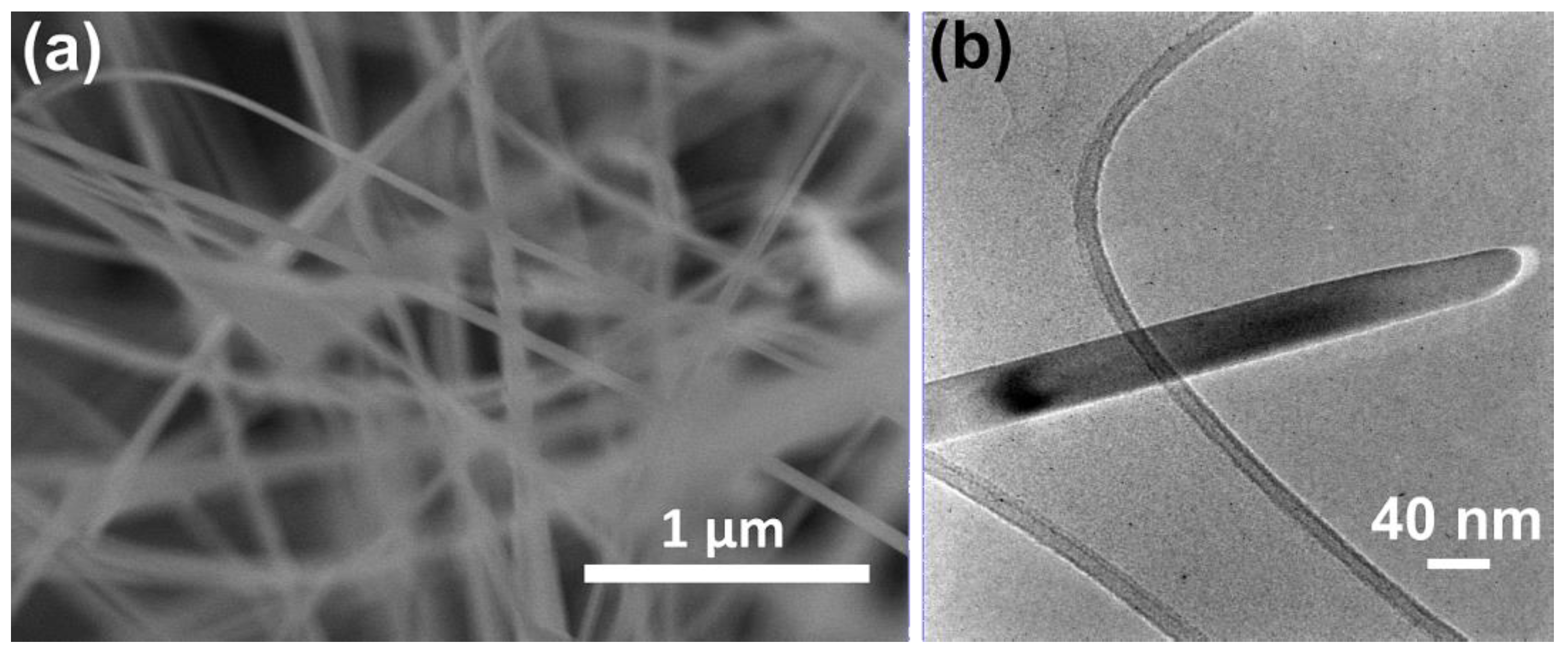
2.2. Nanowires Characterization

The morphology of the metal oxide nanowires was investigated by scanning electron microscopy (SEM) with a Hitachi S-4800 (Tokyo, Japan) and by transmission electron microscopy (TEM) using a JEM-100CX (JEOL, Tokyo, Japan) operating at 90 kV. The structure of the SnO₂ nanowires was characterized by X-ray diffraction (XRD) using a Philips Xpert Pro (Malvern Panalytical, Malvern, UK) diffractometer working at 40 kV with CuKα radiation.

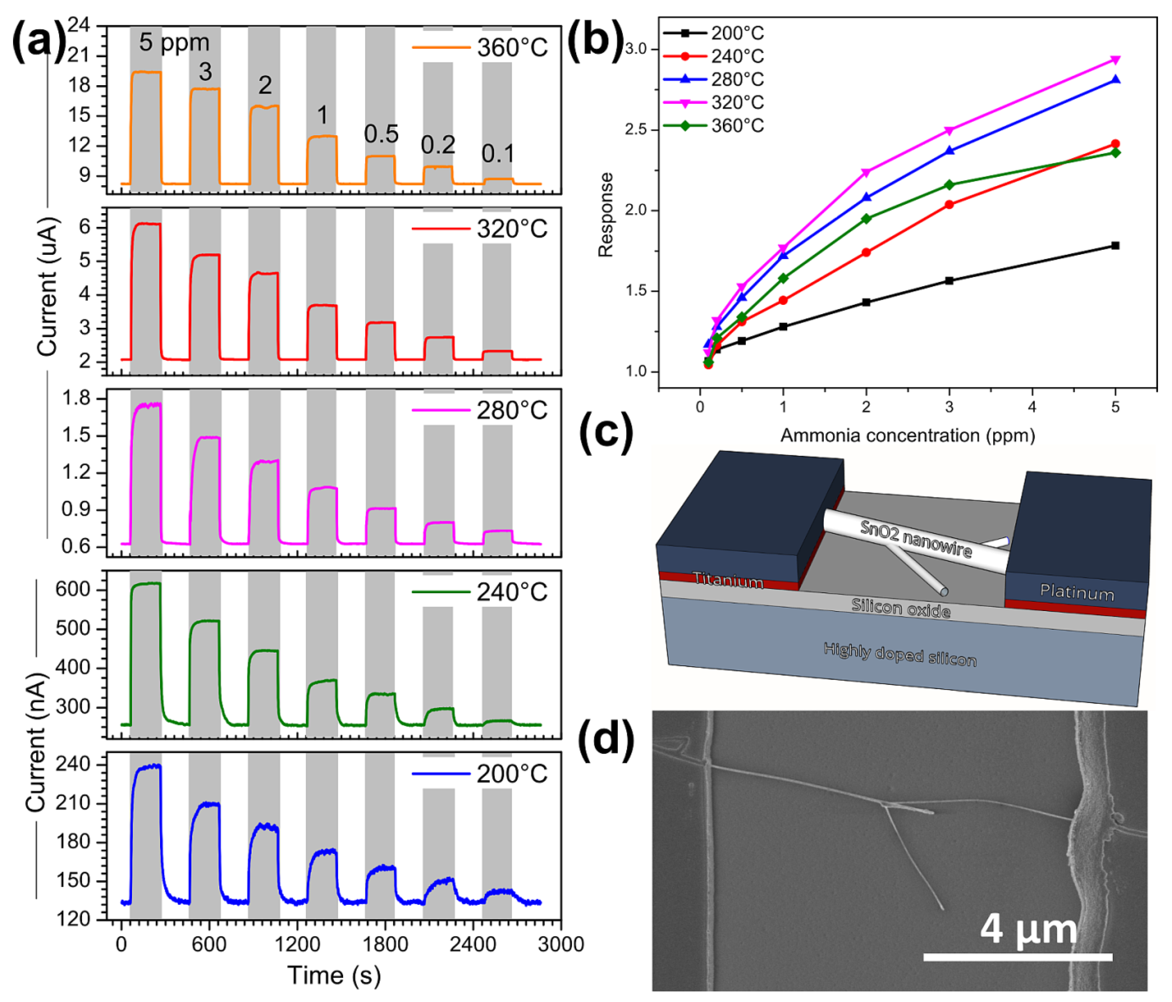
2.3. Sensor Fabrication

A piece of a substrate with grown SnO₂ nanowires was then treated under ultrasounds in dimethylformamide (DMF) for two seconds. Some drops of the resulting dispersion were spread on an entire Si/SiO₂ wafer while spinning it at 6000 rpm, in order to optimize the nanowire density. A Ti/Pt (10/250 nm) two-dimensional array composed of square electrodes was deposited on top of the dispersed nanowires using sputtering and UV lithography on the whole wafer. Titanium was used as an adhesion layer in this case, but this choice must be weighed in light of its influence on the performance of the device [16,17,18]. By observing the gap between all the pairs of electrodes under an optical microscope and measuring their resistance, pairs of electrodes bridged by one or more nanowires were found. Observing the candidates with the best characteristics by means of SEM microscopy, the pairs were verified in order to choose the single nanowire devices and check their characteristics (arrangement, length, morphology, diameter, etc.).

2.4. Gas Sensor Measurements

A single nanowire sensor was placed on a small heatable plate in a chamber connected to gas flow controllers connected to high purity gas cylinders. The electrodes were contacted with microprobes connected, through a multimeter (Keithely 2410, Cleveland, OH, USA), to a data acquisition program (LabView, National Instruments, Austin, TX, USA). The sensor was initially heat-treated for 8 h at 500 °C in nitrogen while being fed with 1 V, in order to stabilize the structure and its resistance so that they do not change during the experiments [19]. The sensor showed good ohmic contact between the nanowire and the metal electrodes and its resistance dropped from 7.5 MOhm at 200 °C down to 122 kOhm at 360 °C. The sensor was initially tested with different ammonia concentrations (5 to 0.1 ppm) while heated to various temperatures (200–360 °C).

The most common definition in the literature has been used for the sensor response, that is S = R_air/R_NH3, where R_air and R_NH3 are, respectively, the resistance of the sensor in air and in the presence of ammonia. The speed of the single nanowire sensor is evaluated using a common definition of response and recovery times: t_RESP is the time it takes to reach 90% of the maximum response, and t_REC is the time to go down to 90% of the full recovery. The limit of detection (LoD), that is, the minimum detectable concentration, was calculated as 3 • N/D, where N is the noise of the sensor signal (its standard deviation) in air, and D is the derivative of the sensor response as a function of the ammonia concentration.

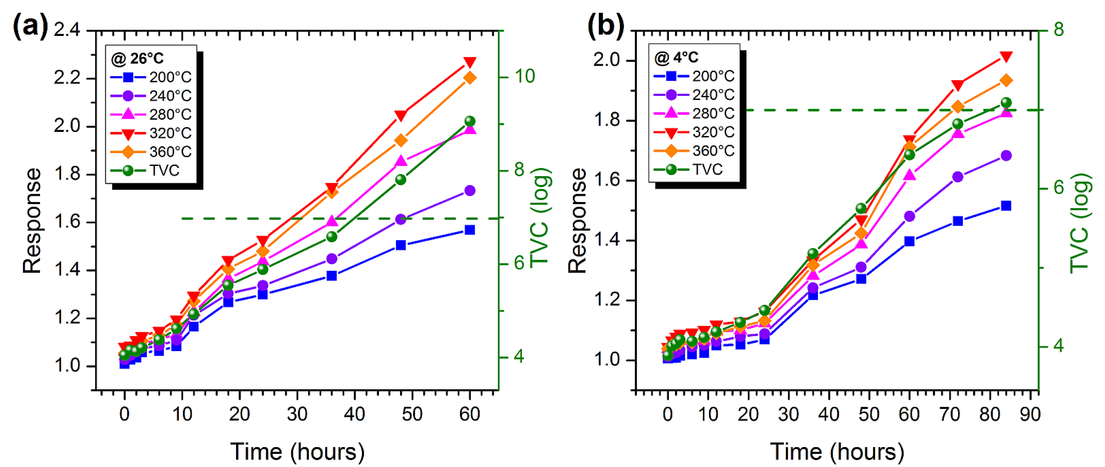
2.5. Meat and Fish Spoilage Measurement

The two foods (one marble trout and one piece of pork) were cut into cubes weighing about 20 g from a larger fresh piece, using disposable gloves and autoclaved tools. Each sample was stored individually, in a glass jar, until the moment of measurement. A part of the samples was stored at room temperature (about 26 °C) and another part instead in a refrigerator at a temperature of 4 °C. At each measurement (initially every hour, then 3, 6, and finally 12 h) a sample was placed in the measurement chamber to determine the response of the gas sensor, and immediately afterward, it was subjected to microbial analysis, in order to compare the two measurements. The total viable count (TVC) was assessed using a spread plate method [20] on a plate count agar and agar base (Oxoid CM0463 and 0055). The plates were then counted after an incubation time of 48 h at 30 °C.

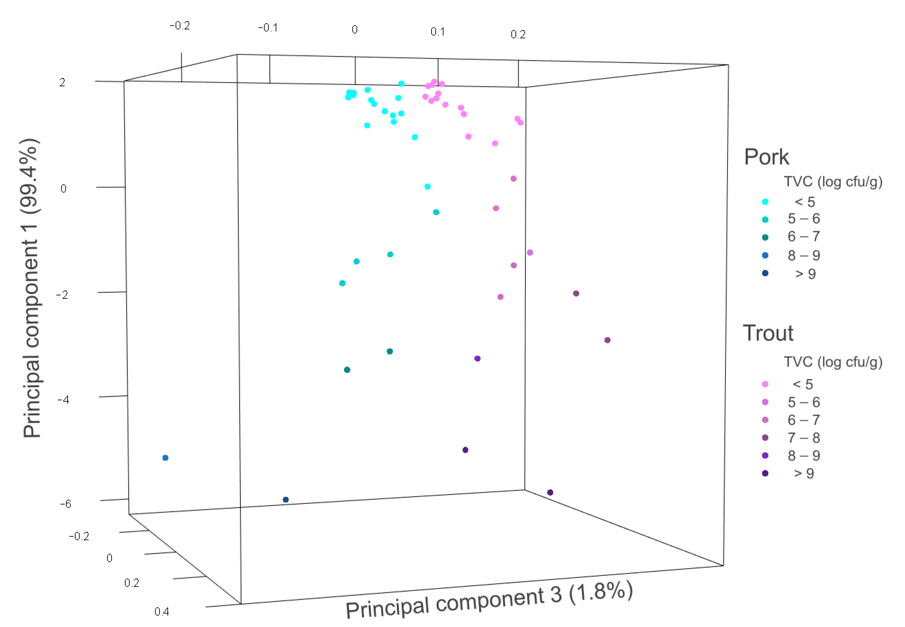
2.6. Machine Learning

Since the single response of the resistive sensor is inherently non-selective, the responses at the five working temperatures were combined to create 5-dimensional points that could be processed and analyzed with multivariate statistical analysis techniques [21]. The 5D points were used both for visualization via principal component analysis (PCA) and for classification and quantification with a support vector machine (SVM). The samples used for PCA are those measured initially, to monitor the degradation of the samples over time. Subsequently, other samples were randomly measured in order to reach a sufficient number of data to be divided into two groups: two-thirds for the training group and one-third for the test group. The SVM was used as a classifier in two successive steps: a first classifier was used to identify whether the sample is fish or meat (marble trout or pork), and subsequently, two classifiers were used on the subgroups identified as fish and meat, in order to evaluate their degree of freshness. All SVM classifiers were always used with a linear kernel.

3. Results and Discussion

3.1. Nanowires Characterization

The SnO₂ nanowire forest was initially studied by scanning electron microscopy in order to investigate the morphology of the nanostructures. The nanowires that make up the forest, shown in Figure 1a, have diameters around 40–65 nm and are several microns long. Many of the nanowires shown are blurred due to the charging effect due to their high electrical resistance.

The TEM image in Figure 1b shows the tip of a single nanowire on a carbon membrane. The nanowire is straight and with a constant diameter. The structure of the nanowires was investigated through X-ray diffraction. All peaks shown in the X-ray pattern of Figure 2 (black, top) can be easily indexed as the tetragonal phase of SnO₂, with lattice parameters of a = b = 4.742 and c = 3.186 Å, which are in good agreement with the values reported as reference (JCPDS n. 77-0450, red, bottom).

There are no phases other than the tetragonal one of SnO₂, nor peaks due to impurities or amorphous contributions, confirming the good crystallinity of the nanowires.

3.2. Ammonia Sensing Performance

The sensing properties of the single nanowire sensor were initially tested by measuring different concentrations of ammonia, as this volatile is part of the TVB-N, which is a known marker of meat and fish degradation [22]. Low concentrations were measured, from 5 to 0.1 ppm. The measurements were carried out at five different temperatures, from 200 to 360 °C, in order to subsequently combine the obtained responses and process the data with multivariate statistical analysis. Figure 3a shows the current as a function of time as the different ammonia concentrations (indicated by the gray background) is injected into the measurement chamber. As can be seen, as the ammonia is flowed onto the nanowire, the current rapidly increases and quickly returns to its base value as the ammonia is evacuated.

As can be seen in Figure 3a, the sensor is very stable after the heat treatment carried out before the measurements. It can be seen in the figure that both the response and the recovery become faster as the working temperature of the sensor increases. Average response times decrease from 48 to 8 s, while average recovery times decrease from 43 to 6 s. Figure 3b shows the response values for the various ammonia concentrations at the five working temperatures. As can be seen, the response increases with increasing gas concentration with a slightly less than a linear trend in most cases. The response at the lowest temperature is the most linear, while the response to the highest temperature is the one that tends toward saturation. Figure 3c shows a three-dimensional diagram of the sensor, with the SnO₂ nanowire (in white) acting as a bridge between the two metal electrodes (in blue). Figure 3d instead shows a top view SEM image of the nanowire constituting the sensor. The behavior shown in Figure 3a, with the current increasing as ammonia is injected, is typical of n-type semiconductors in response to reducing gases. Tin oxide is in fact a semiconductor in which the charge carriers are electrons, and it is very sensitive to the atmosphere that surrounds it [23], especially to reducing gases such as ammonia [24]. When the sensor is exposed to air, the oxygen reacts on the surface of the SnO₂ by draining electrons from the nanowire, thus decreasing the current flowing through it. The ammonia molecules, on the other hand, react with the oxygen absorbed on the surface, releasing the electrons in the nanowire and thus increasing the current flowing through it [25,26].

2 NH₃ + 3 O⁻(ads) → N₂ + 3 H₂O + 3 e⁻

(1)

The last parameter calculated regarding the ammonia detection performance is the limit of detection, calculated according to the definition given in Section 2.4. The calculated value decreases with increasing temperature, from 70 ppb at 200 °C to 18 ppb at 360 °C. This very low value is important for the sensor to detect the low concentrations present in the early stages of meat and fish degradation.

3.3. Measurements on Marble Trout and Pork Samples

The sensor response and the total viable count measured on marble trout samples stored at room temperature are plotted in Figure 4a. The response of the sensor at any working temperature increases over time, as does the microbial count. The total viable count increases its slope after about 10 hours and reaches the threshold value after about 23 h. This value, indicated by the dashed horizontal green line, is considered the consumability limit of the sample in the literature [9,27] and for health regulations [28].

A similar behavior is observed in Figure 4b, which shows the sensor responses and the total viable count measured on marble trout samples stored in a refrigerator at 4 °C. In this case, the curves rise more slowly, and the microbial count reaches the threshold value after about 66 h. In both cases, the response of the gas sensor at various temperatures follows the curve of the TVC quite closely. This good correlation, already demonstrated elsewhere [29], shows that the response of the resistive sensor can be used as an indirect measure of the microbial count and therefore of the state of degradation of the food sample.

Figure 5a shows the sensor response and total viable count measured on pork samples stored at room temperature. Additionally, in this case, the curves increase over time, demonstrating the progressive degradation of the meat. The TVC graph increases the slope after about 10 hours and reaches the consumability threshold after about 40 h.

Figure 5b shows the resistive sensor response and TVC of pork samples stored in a refrigerator at 4 °C. The slope of the curves is low up to about 24 h and then increases, and the microbial count reaches the threshold after about 80 h.

3.4. Distinction between Meat and Fish

In the previous section, we saw that the response of the resistive gas sensor, at any working temperature, could be used as an indirect measure of the total viable count, both on marble trout and pork samples. Unfortunately, the sensor response lends itself to calibration for only one sample type and could not be used to distinguish different food samples. For this reason, the responses at five different temperatures were combined and processed through multivariate statistical analysis. Initially, we used principal component analysis to visualize the relationship between meat and fish points over time. The aim was to investigate whether the two foods had two different trends and observe whether the samples stored at different temperatures differed in any way. The results are shown in Figure 6, where the top samples are those measured initially (at the beginning of the plots in Figure 4 and Figure 5), and then the points drop down as time passes.

The position of the points is given by the PCA of the 5D points obtained by combining the responses collected at various temperatures, while their color reflects the TVC measurement. Moving down the principal component 1 (vertically), the points become darker, indicating a higher TVC (legend on the right in the figure) and therefore greater degradation as time passes, as expected. The two groups of points, relating to fish and meat, are easily distinguishable, and rather separate from each other. This is a good indication that they are classifiable. Unfortunately, however, it is not possible to distinguish between samples stored in the refrigerator and those stored at room temperature.

Based on these results, a support vector machine was then used to classify the fish and meat samples. This algorithm first uses a data set to map the five-dimensional space according to the classes and then compares the new data with the map to classify them. The results of this classification are shown in the confusion matrix in

Table 1. Confusion matrix of the classification between meat and fish using the single nanowire gas sensor.

	True
Estimated	Sample	Pork	Trout
	Pork	20	1
	Trout	1	20

.

For both meat and fish, the sensor correctly classified 20 out of 21 samples tested for 95.2% accuracy. The two misclassified points were both related to degraded food samples, with TVC greater than or close to 8.

3.5. Estimation of the Degree of Freshness of Food

Once the sensor distinguished the samples by type (marble trout or pork), the points relating to the two foods were processed with two other classifiers based on support vector machines, one for fish and one for meat. In this case, instead of using the “food type” label of the training dataset points (as the classifier used previously), the “degree of freshness” label was used, which was assigned according to the TVC value. The classification results for the pork samples are shown in the confusion matrix in

Table 2. Confusion matrix of classification regarding the state of freshness of pork samples. The background color represents the extent of the severity of a possible misclassification.

Pork		Estimated TVC (log cfu/g)
		<5	5–6	6–7	7–8	8–9	>9
True TVC (log cfu/g)	<5	9
	5–6		4
	6–7			2
	7–8				2
	8–9		1			2
	> 9						1

.

The sensor classified the degree of freshness of pork samples very well, with an accuracy of 95.2%. Only one sample was classified in the wrong degree of freshness, which was called pork, while in reality, it was a sample of marble trout. Unfortunately, as can be seen from the background color of the misclassified sample cell, the error is significant, as the sample is considered fresh, while in reality, it is rather degraded. Evidently, the misclassification in the previous step has strong repercussions on the results of this classification.

The estimate of the degree of freshness of the marble trout samples is shown in

Table 3. Confusion matrix of classification regarding the state of freshness of marble trout samples. The background color represents the extent of the severity of a possible misclassification.

Marble Trout		Estimated TVC (log cfu/g)
		<5	5–6	6–7	7–8	8–9	> 9
True TVC (log cfu/g)	<5	9
	5–6		3
	6–7			2
	7–8			1	2	1
	8–9						1
	>9						2

.

It is immediately evident that the classification, in this case, is worse, as three samples are incorrectly classified, for an accuracy of 85.7%. One of the three misclassified samples is the one that was incorrectly classified in the previous step and is, therefore, in reality, a pork sample. While three misclassified samples may appear to be a considerable number, we have to consider different degrees of severity of the misclassifications. In fact, the only major error is that which estimates a degraded sample as fresh. In the other two cases, however, degraded samples were evaluated as even more degraded and therefore were minimal errors. The severity is highlighted in the table by the background color: a green background means that fresh samples are still considered fresh, and degraded samples are considered degraded, even if with different freshness classes (misclassification without consequences). A yellow background means that a fresh sample is considered degraded and would therefore lead to food waste. Finally, a red background color means that a degraded sample is considered fresh, which could lead to food poisoning. Given these considerations, we can state that the sensor makes 1 important error on the 21 samples of pork and 1 major error on the 21 samples of marble trout. In both cases, therefore, the system estimates the freshness of the food with an accuracy of 95.2%. If, on the other hand, we consider all types of errors, including those without repercussions, then the system estimates the freshness of pork and marble trout with an accuracy of 95.2 and 85.7%, respectively. It should be emphasized that these results were obtained from a single trout and a single piece of pork. We expect that testing samples from more than one animal of each type, the uncertainty of the measurement may increase. On the other hand, the greater number of samples would help train the support vector machine better, and this should improve performance. The balance between these two effects will be evaluated in future work. In any case, considering the small size and low cost of the device, this performance indicates that the single nanowire gas sensor may be a candidate as a fast and non-invasive method of estimating the freshness of meat and fish.

4. Conclusions

A single SnO₂ nanowire, used as a resistive sensor, allows the evaluation of the freshness of different foods. By combining the sensor responses at five different temperatures and processing them with multivariate statistical analysis (PCA) and machine learning (SVM) techniques, the sensor is able to distinguish between marble trout and pork samples and to estimate their state of freshness. The sensor recognized the type of sample (meat or fish) in 95.2% of cases. Furthermore, it recognized the degradation status in 90.5% of cases (85.7% of cases for trout and 95.2% of cases for pork). Considering that in several cases, the misclassification had no repercussions, as it considered the degraded samples even more degraded, the sensor overall recognized whether the sample was edible in 95.2% of cases. Considering the size (less than a square millimeter), the low cost, the speed, and the non-invasiveness, the gas sensor is proven to be ideal as a monitoring tool along the meat and fish production and distribution chain.

References

1. Scharff, R.L. Economic burden from health losses due to foodborne illness in the United States. J. Food Prot. 2012, 75, 123–131. [Google Scholar] [CrossRef]
2. Sundström, K. Cost of Illness for Five Major Foodborne Illnesses and Sequelae in Sweden. Appl. Health Econ. Health Policy 2018, 16, 243–257. [Google Scholar] [CrossRef] [Green Version]
3. Boyer, D.; Ramaswami, A. Comparing urban food system characteristics and actions in US and Indian cities from a multi-environmental impact perspective: Toward a streamlined approach. J. Ind. Ecol. 2020, 24, 841–854. [Google Scholar] [CrossRef]
4. Comi, G. (Ed.) Spoilage of Meat and Fish. In The Microbiological Quality of Food; Elsevier: Amsterdam, The Netherlands, 2017. [Google Scholar] [CrossRef]
5. Wojnowski, W.; Majchrzak, T.; Dymerski, T.; Gębicki, J.; Namieśnik, J. Portable Electronic Nose Based on Electrochemical Sensors for Food Quality Assessment. Sensors 2017, 17, 2715. [Google Scholar] [CrossRef] [PubMed] [Green Version]
6. Deisingh, A.K.; Stone, D.C.; Thompson, M. Applications of electronic noses and tongues in food analysis. Int. J. Food Sci. Technol. 2004, 39, 587–604. [Google Scholar] [CrossRef]
7. Chang, L.-Y.; Chuang, M.-Y.; Zan, H.-W.; Meng, H.-F.; Lu, C.-J.; Yeh, P.-H.; Chen, J.-N. One-Minute Fish Freshness Evaluation by Testing the Volatile Amine Gas with an Ultrasensitive Porous-Electrode-Capped Organic Gas Sensor System. ACS Sens. 2017, 3, 531–539. [Google Scholar] [CrossRef]
8. Perez de Vargas-Sansalvador, I.M.; Erenas, M.M.; Martinez-Olmos, A.; Mirza-Montoro, F.; Diamond, D.; Capitan-Vallvey, L.F. Smartphone based meat freshness detection. Talanta 2020, 216, 120985. [Google Scholar] [CrossRef] [PubMed]
9. Leng, T.; Li, F.; Chen, Y.; Tang, L.; Xie, J.; Yu, Q. Fast quantification of total volatile basic nitrogen (TVB-N) content in beef and pork by near-infrared spectroscopy: Comparison of SVR and PLS model. Meat Sci. 2021, 180, 108559. [Google Scholar] [CrossRef] [PubMed]
10. Olafsdóttir, G.; Martinsdóttir, E.; Oehlenschläger, J.; Dalgaard, P.; Jensen, B.; Undeland, I.; Mackie, I.M.; Henehan, G.; Nielsen, J.; Nilseng, H. Methods to evaluate fish freshness in research and industry. Trends Food Sci. Technol. 1997, 8, 258–265. [Google Scholar] [CrossRef]
11. Thai, N.X.; Van Duy, N.; Hung, C.M.; Nguyen, H.; Tonezzer, M.; Van Hieu, N.; Hoa, N.D. Prototype edge-grown nanowire sensor array for the real-time monitoring and classification of multiple gases. J. Sci. Adv. Mater. Devices 2021, 5, 409–416. [Google Scholar] [CrossRef]
12. Zeng, H.; Zhang, G.; Nagashima, K.; Takahashi, T.; Hosomi, T.; Yanagida, T. Metal-oxide nanowire molecular sensors and their promises. Chemosensors 2021, 9, 41. [Google Scholar] [CrossRef]
13. Tonezzer, M.; Thai, N.X.; Gasperi, F.; Van Duy, N.; Biasioli, F. Quantitative Assessment of Trout Fish Spoilage with a Single Nanowire Gas Sensor in a Thermal Gradient. Nanomaterials 2021, 11, 1604. [Google Scholar] [CrossRef] [PubMed]
14. Thai, N.X.; Tonezzer, M.; Masera, L.; Nguyen, H.; Duy, N.V.; Hoa, N.D. Multi gas sensors using one nanomaterial, temperature gradient, and machine learning algorithms for discrimination of gases and their concentration. Anal. Chim. Acta 2020, 1124, 85–93. [Google Scholar] [CrossRef] [PubMed]
15. Redwing, J.M.; Miao, X.; Li, X. Vapor-Liquid-Solid Growth of Semiconductor Nanowires. In Handbook of Crystal Growth, 2nd ed.; Thomas, F.K., Ed.; Elsevier: Amsterdam, The Netherlands, 2015; Volume 3, pp. 399–439. [Google Scholar]
16. Lin, Y.-F.; Jian, W.-B. The impact of nanocontact on nanowire based nanoelectronics. Nano Lett. 2008, 8, 3146–3150. [Google Scholar] [CrossRef]
17. Todeschini, M.; Bastos da Silva Fanta, A.; Jensen, F.; Birkedal Wagner, J.; Han, A. Influence of Ti and Cr Adhesion Layers on Ultrathin Au Films. ACS Appl. Mater. Interfaces 2017, 9, 37374–37385. [Google Scholar] [CrossRef] [Green Version]
18. Zeng, H.; Takahashi, T.; Kanai, M.; Zhang, G.; He, Y.; Nagashima, K.; Yanagida, T. Long-Term Stability of Oxide Nanowire Sensors via Heavily Doped Oxide Contact. ACS Sens. 2017, 8, 1854–1859. [Google Scholar] [CrossRef] [PubMed]
19. Tischner, A.; Maier, T.; Stepper, C.; Köck, A. Ultrathin SnO2 gas sensors fabricated by spray pyrolysis for the detection of humidity and carbon monoxide. Sens. Actuators B Chem. 2008, 134, 796–802. [Google Scholar] [CrossRef]
20. López, A.; Baguer, B.; Goñi, P.; Rubio, E.; Gómez, J.; Mosteo, R.; Ormad, M.P. Assessment of the methodologies used in microbiological control of sewage sludge. Waste Manag. 2019, 96, 168–174. [Google Scholar] [CrossRef]
21. Tonezzer, M.; Izidoro, S.C.; Moraes, J.P.A.; Dang, L.T.T. Improved Gas Selectivity Based on Carbon Modified SnO2 Nanowires. Front. Mater. Sci. 2019, 6, 277. [Google Scholar] [CrossRef]
22. Bekhit, A.E.A.; Holman, B.W.B.; Giteru, S.G.; Hopkins, D.L. Total volatile basic nitrogen (TVB-N) and its role in meat spoilage: A review. Trends Food Sci. Technol. 2021, 109, 280–302. [Google Scholar] [CrossRef]
23. Tsuda, N.; Nasu, K.; Fujimori, A.; Siratori, K. Electronic Conduction in Oxides, 2nd ed.; Springer: Berlin/Heidelberg, Germany, 2000. [Google Scholar]
24. Marikutsa, A.; Rumyantseva, M.; Gaskov, A. Selectivity of catalytically modified tin dioxide to CO and NH3 gas mixtures. Chemosensors 2015, 3, 241–252. [Google Scholar] [CrossRef] [Green Version]
25. Wagh, M.S.; Jain, G.H.; Patil, D.R.; Patil, S.A.; Patil, L.A. Modified zinc oxide thick film resistors as NH3 gas sensor. Sens. Actuators B Chem. 2005, 115, 128–133. [Google Scholar] [CrossRef]
26. Wu, H.; Ma, Z.; Lin, Z.; Song, H.; Yan, S.; Shi, Y. High-Sensitive Ammonia Sensors Based on Tin Monoxide Nanoshells. Nanomaterials 2019, 9, 388. [Google Scholar] [CrossRef] [PubMed] [Green Version]
27. Koutsoumanis, K. Predictive Modeling of the Shelf Life of Fish under Nonisothermal Conditions. Appl. Environ. Microbiol. 2001, 67, 1821–1829. [Google Scholar] [CrossRef] [PubMed] [Green Version]
28. Sciortino, J.A.; Ravikumar, R. Chapter 5: Fish Quality Assurance. In Fishery Harbour Manual on the Prevention of Pollution, Bay of Bengal Programme; Bay of Bengal Programme: Madras, India, 1999. [Google Scholar]
29. Tonezzer, M. Detection of Mackerel Fish Spoilage with a Gas Sensor Based on One Single SnO2 Nanowire. Chemosensors 2021, 9, 2. [Google Scholar] [CrossRef]
Figure 1. (a) SEM image of the SnO2 nanowires forest; (b) TEM image of a nanowire tip.
Chemosensors 09 00249 g001
Figure 2. XRD patterns: top (black): experimental pattern of the SnO2 nanowires used to fabricate the single-nanowire sensor; bottom (red online): reference pattern of tetragonal SnO2 (JCPDS 77-0450).
Chemosensors 09 00249 g002
Figure 3. (a) dynamic current at different temperatures during the injection of different ammonia concentrations; (b) sensor response as a function of gas concentration at different temperatures; (c) three-dimensional model of the single nanowire sensor; (d) SEM image of the single nanowire sensor.
Chemosensors 09 00249 g003
Figure 4. (a) Sensor response (colored symbols, left scale) and bacterial population (green spheres, right scale) in marble trout samples stored at room temperature over a period of 60 h; (b) sensor response (colored symbols, left scale) and bacterial population (green spheres, right scale) in fresh marble trout stored at in a refrigerator over a period of 72 h.
Chemosensors 09 00249 g004
Figure 5. (a) Sensor response (colored symbols, left scale) and bacterial population (green spheres, right scale) in pork samples stored at room temperature over a period of 60 h; (b) sensor response (colored symbols, left scale) and bacterial population (green spheres, right scale) in fresh marble trout stored at in a refrigerator over a period of 84 h.
Chemosensors 09 00249 g005
Figure 6. Principal component analysis of meat and fish samples over time. Shades of blue (cyan to navy) indicate points for pork samples, while shades of purple (pink to violet) indicate points for marble trout samples.
Chemosensors 09 00249 g006