Applications of the Photoionization Detector (PID) in Occupational Hygiene. Estimation of Air Changes per Hour in Premises with Natural Ventilation

Abstract

The importance of ventilation in closed workplaces increased after the onset of the COVID-19 pandemic. New methodologies for measuring the number of air changes per hour (ACH) in a premise where natural ventilation is applied are necessary. It is demonstrated how the ionic photoionization detector (PID) can be employed for tracer gas decay methodology using a volatile organic solvent (acetone). The methodology applied to calculate ACH in a naturally ventilated room, with various combinations of door and window openings, provides ACH values of between 2 and 17 h⁻¹. Two classrooms were studied to verify if the minimum ventilation requirements recommended by official guidelines were met. The values for ACH on different days varied, mainly between 15 and 35 h⁻¹, with some exceptional values higher than 40 h⁻¹ on very windy days. These results agree with the quality air data recorded by the installed CO₂ sensors, ensuring adequate hygienic conditions for the users of the rooms. The fast response of the PID allows the measurement of different locations in the room during the same assay, which provides additional information regarding the air distribution inside during the ventilation process. This methodology is fast and easy, and the necessary equipment is simple to obtain and use routinely, whether it is needed to measure several rooms or to monitor one room periodically.

1. Introduction

The ventilation of workplaces, renewing the interior air, is a necessity to maintain an environment with adequate air quality. Even without the presence of chemical agents in the workplace, the breathing of the occupants of a room, as well as the diffuse emissions from the objects in it, require the renewal of air to eliminate CO₂, water vapor, unpleasant odors, aerosols, and possible volatile organic compounds.

Air pollution is a serious threat to human health, causing millions of deaths each year (about 4,900,000 in 2017 alone) [1]. Specifically, indoor air-pollution-based illnesses include sick building syndrome (SBS) and building-related illness (BRI) [2]. In addition, evidence suggests that the pandemic caused by the severe acute respiratory syndrome coronavirus 2 (SARS-CoV-2), responsible for the COVID-19 disease, can spread from an infected person’s mouth or nose in small liquid particles when the person coughs, sneezes, sings, breathes or talks, by inhalation or inoculation through the mouth, nose or eyes. These liquid particles are different sizes, ranging from larger ‘respiratory droplets’ to smaller ‘aerosols.’ The virus spreads mainly between people who are in close contact with each other, typically within 1 m (short-range), and can also spread to others through aerosols at longer (beyond 1 m) distances. The risk of long-distance aerosol transmission is higher in poorly ventilated and/or crowded indoor settings where people spend long periods [3].

These facts increased the need for improved premise ventilation, along with additional preventive measures, such as facemask use. Various agencies developed guidelines establishing minimum air renewal values to minimize the chances of contagion, and some studies related to natural ventilation as a COVID-19 prevention measure were published [4]. In Spain, air quality requirements in educational establishments are set by the Regulation on Thermal Installations in Buildings (RITE) [5]. Different types of air quality are defined, and a quality of indoor air IDA 2 (good quality air) must be achieved in classrooms. Various methodologies are proposed to verify the compliance with these requirements, such as an outdoor air supply of 12.5 L/s/person (45 m³/h/person) or a maximum concentration of 500 ppm of CO₂ over the external concentration (usually about 400 ppm).

In 2020, the Spanish National Research Council, CSIC, developed a guide for ventilation in classrooms to reduce the likelihood of airborne COVID-19 infection. An adequate value to reduce the risk of contagion was at least 14 L/s/person [6].

For all these reasons, measuring the ventilation of a closed premise is necessary for health and hygienic control. The most employed method is to use a tracer gas, based on a mass balance of the tracer gas in the in air, and measure its evolution over time under different methodologies [7,8,9].

Among all the possible methodologies, tracer decay is the most used [10]. A known amount of the gas is diffused in the test space, in the absence of ventilation, until a constant concentration is reached. Its evolution in time is measured when ventilation is started, and these data can be treated to calculate the air changes per hour (ACH) value. These methods are more adapted to natural ventilation in situ measurements, with an accuracy of about 15% [11].

In addition, other measuring options can be employed. In the pulse technique, a steady-state variant of the tracer decay technique, the measurement period starts before the tracer is injected, but in this case, the total volume of the tracer gas must be known. In the constant injection technique, the tracer gas is injected constantly in the system, and usually, the measurement ends when a steady state is reached. However, biased results can be obtained if ventilation is not constant. Finally, in the constant concentration approach, an active control system is used to inject an adequate amount of tracer gas to maintain the concentration of tracer at a predefined value. Other methodologies also exist, for example, using commercial, passive, indoor air quality samplers and a careful planning phase to account for imperfect mixing [12].

Regarding the ideal tracer gas, it must exhibit some important properties, although no tracer gas completely fulfils all of these properties. Some of these properties are safety, non-reactivity, insensibility, uniqueness and measurability.

Although several gases were proposed historically, only two of them are now employed [8]. Sulfur hexafluoride, SF₆, is odorless, non-flammable and has a low toxicity. However, it is an expensive gas, sold as a liquefied compressed gas, with a high molecular weight, and thus a higher density compared to air; this means that both its manipulation and homogeneous mixing are difficult. In addition, it is included in the Kyoto protocol and requires expensive equipment for its measurement (usually a photoacoustic infrared detector) [13]. For all of these reasons, the use of this compound is set to disappear from laboratories.

CO₂ also has a low toxicity and is easy to obtain, although it is also difficult to handle, both in its gaseous and solid form (very low temperatures cause losses during handling and cold burns). Its measurement is easy with specific sensors, most of them based on IR radiation absorption, but its disadvantage is its presence in the inlet gas (concentrations of around 400 ppm or higher, and not always constant depending on the quality of the outside air), which complicates calculations and may cause errors if these concentrations change over time. This can easily occur, especially in urban environments (traffic, heating, etc.) or if other persons are close to the measurement location. For example, in our campus, external values ranging from 404 to 574 ppm of CO₂ were measured, likely due to the close presence of a highway.

For these reasons new options for the real-time measurement of a compound intentionally added to air are of great interest for ACH calculations. One of these options is the photoionization detector, PID, an instrument for real-time gas measuring which has several advantages.

In a PID, the gas or vapor is ionized by a short-wavelength ultraviolet (UV) lamp. Substances with ionization potentials lower than the energy emitted by the lamp are ionized and generate a current at the collector, which is proportional to the number of ionized species. These processes last femtoseconds to milliseconds, and are very interesting for industrial hygiene and safety measurements. The response time of PID instruments is usually from a few to several seconds, mainly due to the rate at which the sample is pumped through the detection chamber and flushed completely. Usually a PID has only one lamp, although lamps can be exchanged depending on the compound selectivity required. The most common lamp is the 10.6 eV lamp, comprising a krypton fill gas and a magnesium fluoride window. PID is a non-specific measurement technique, so mixtures of compounds provide a weighted total response of all detectable compounds. Still, some papers describe its utility for solvent mixtures [14]. The most common matrix gases (hydrogen, helium, argon, carbon dioxide, butane, chlorofluorocarbons, nitrogen, and methane) do not respond to the PID themselves, although they may affect the response to detectable vapors.

Compounds with ionization energy <10.6 eV (or the energy of the lamp) are measurable by PID, and those with a lower ionization energy are generally more sensitive. They are usually used to detect volatile organic compounds (VOCs), and aromatics, olefins, ketones, ethers, amines, and organic sulfides are among the most sensitive measurable compounds.

The detector is calibrated to produce a reading in a compound air concentration. The most common calibration gas is isobutylene, but any compound can be directly measured if the correction factor for the desired compound and isobutylene are known [15].

In this work a PID was proposed to determine ACH using the tracer decay methodology, considering its advantages for field measurements. Several compounds were studied as tracer agents, and acetone was finally selected. Several advantages over the use of CO₂ as a tracer gas were observed, as a longer concentration interval and lower dependence of the outdoor concentration. The fast response of the instrument allows the researcher to measure several locations simultaneously.

2. Materials and Methods

All the reagents used were of analytical grade.

A photoionization detector PhoCheck TIGER, from Ion Science Ltd. (Fowlmere, Cambridge, UK) was employed for environmental measurements. It was provided with intrinsic safety for the detection of VOCs. A lamp of 10.6 eV was used for the ionization of the VOCs. The response time was lower than 2 s, and the accuracy was ±5%. Data were recorded every second.

The assays were performed in different rooms. All the rooms used to measure the ACH values were located in the Faculty of Chemistry, University of Valencia. Figure 1 shows a blueprint of the building. Room 2.4 was an empty room located on the second floor of the bottom block, with a size of 35 m² and a volume of 105 m³, with one outside wall and covered with four sliding windows of two different sizes. The other two classrooms (1.4 and 1.5) were located at the upper left corner of the first floor of the top building of the Faculty. They formed a right angle, with two outside walls, and the longest wall covered with eight equal sliding windows. Both were very similar in size (108 and 109 m²), with a volume of 285 m³. Apart from the orientation, the main difference was that one of the classrooms had one door (room 1.5) and the other had two doors (room 1.4).

During the course hours, all the plant windows and doors were open, facilitating the ventilation of the floor and making it less sensitive to the wind direction.

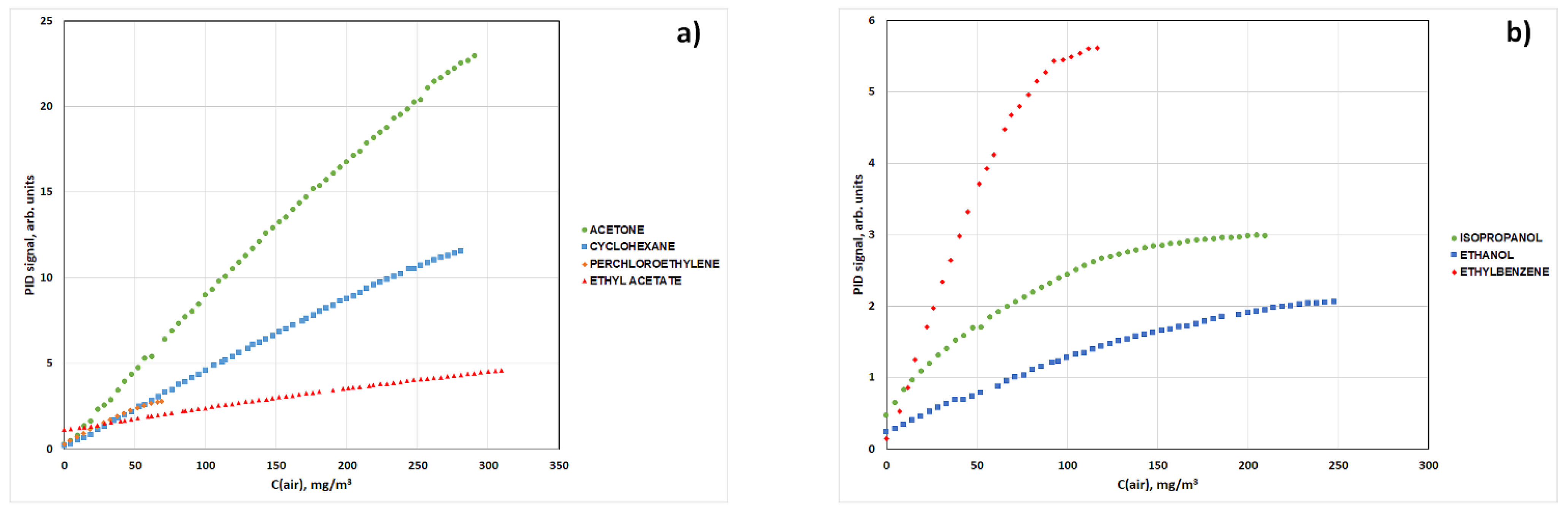
2.1. Selection of the Best Compound

The PID was factory calibrated with isobutylene, and the signal corresponded to ppm of this compound. Although response factors could be used to compare the provided readings with specific gas concentrations (a guide is provided with the instrument), the data were used as they were measured, because a compound with a linear response was selected.

The calibration model for different compounds was studied. These values depended on both the sensibility of the PID and the maximum allowable environmental concentration. The latter was selected according to the threshold limit values (TLV) of the substances.

The seven chemical agents used belonged to six different chemical families: aliphatic (cyclohexane) and aromatic (ethylbenzene) hydrocarbons, alcohols (ethanol and isopropanol), ketones (acetone), esters (ethyl acetate) and organochlorines (tetrachloroethylene); the key properties of these chemical families are summarized in

Table 1. Physicochemical properties and exposure limit values (TLV: threshold limit value; STEL: short-term exposition limit if TLV does not exist; data obtained from Spanish legal values [16]) for the seven substances assayed.

Substance	CAS Number	Vapor Pressure, 20 °C, kPa	Boiling Point, °C	Exposure Limit Values (mg/m3), TLV
Cyclohexane	110-82-7	10.4	81	700
Ethylbenzene	100-41-4	0.95	136	884
Ethanol	64-17-5	5.8	78	1910 (STEL)
Isopropanol	67-63-0	4.3	83	500
Acetone	67-64-1	24	56	1210
Ethyl acetate	141-78-6	9.69	77	734
Tetrachloroethylene	127-18-4	1.9	121	275

.

Measurements were performed on different days of the week to avoid interactions between the chemicals. All the plant windows and doors were kept open, and, during the experiments, the room doors and windows remained closed, and the temperature was almost constant, between 24.5–25.0 °C. The procedure used in each experiment consisted of weighing the chemical agent studied on a scale equipped with a watch glass, placed in the center of the room, and taking into account that the environmental concentration after evaporation should be lower than 50% of the TLV of each agent used. Once weighed, a forced mixing system was used, turning on two oscillating fans in opposite corners of the room to increase the homogenization of the environment under controlled conditions and to achieve a standard well-mixed box (WMB) model [17]. The scale was protected from air gusts to avoid an unstable reading. The PID probe was located away from the source of the chemical agent and protected from air gusts. The data collected in this study (time, evaporated weight, and the signal recorded by the PID) were measured at time intervals resulting from a 0.5 g decrease in the weights recorded by the scale. The data were analyzed by plotting the signal measured by the PID against air concentration (from the mass in grams of the compound that was evaporated). For linear behavior, the slope of the line is the sensibility of the PID to the assayed compound.

For acetone, the total evaporated mass was 30.51 g (equivalent to 290.6 mg/m³, 24% of its TLV). The total evaporation time was about 1 h (58 min).

For cyclohexane, the total evaporated mass was 29.51 g (equivalent to 281 mg/m³, 40% of its TLV value). The total evaporation time was 1 h and 35 min.

For tetrachloroethylene, the total evaporated mass was 7.22 g (equivalent to 68.8 mg/m³, 25% of its TLV value). The total evaporation time was 1 h and 51 min.

For ethyl acetate, the total evaporated mass was 32.46 g (equivalent to 309 mg/m³, 42% of its TLV value). The total evaporation time was 1 h and 23 min.

For isopropanol, the total evaporated mass was 22.03 g (equivalent to 209.8 mg/m³, 42% of its TLV). The total evaporation time was 2 h and 20 min.

For ethanol, the total evaporated mass was 26.00 g (equivalent to 247.6 mg/m³, 13% of its short-term exposition value). The total evaporation time was 2 h and 24 min.

For ethylbenzene, the total evaporated mass was 12.24 g (equivalent to 116.6 mg/m³, 13% of its TLV value). The total evaporation time was 2 h and 55 min.

For the last three compounds, a non-linear behavior was detected. In the three cases, data acquisition stopped when a saturation of the signal was observed.

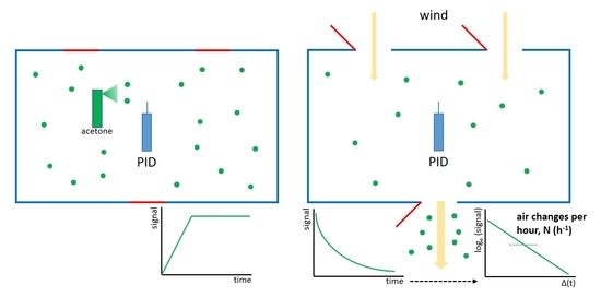
2.2. Use of Acetone and a PID to Calculate the ACH in Different Ventilation Conditions

The possibility of using the data obtained from the PID, using acetone as a tracer gas to calculate the ACH in different situations, was studied.

The tests were performed in the same room as in the previous part. The controlled contaminated atmosphere was prepared by spraying inside the room, with the doors and windows closed, a measured mass of acetone, and waiting for homogenization using two oscillating fans. They were turned off before starting the measuring process. When a stable reading of the PID was obtained in different parts and heights of the room, five different combinations of opened doors and windows were studied. These different combinations were selected to provide increasing values of natural ventilation. The measurements were taken manually every one or two minutes (depending on the ventilation rate) at the four corners of the room, at a height of about 1 m (head position when sitting), to test the efficiency of the ventilation (Figure 1).

Wind speed and wind direction (hourly mean) were taken from an external governmental environmental quality measurement station, located 100 m from the building (https://agroambient.gva.es/va/web/calidad-ambiental/datos-on-line, Burjassot-Facultats measurement point, accessed on 19 November 2021).

2.3. Use of Acetone and a PID to Calculate the ACH in Two Different Classrooms

Finally, in the third part of the experiment, the ACH for two classrooms of the Faculty of Chemistry were measured.

The controlled contaminated atmosphere was prepared as in the previous section, by spraying inside the room, with doors and windows closed, a measured mass of acetone, and waiting for homogenization using two oscillating fans. The fans were turned off before starting the measuring process. When a stable reading of the PID was obtained in different parts and heights of the room, all the windows and doors were opened, as they are used during the classes. The measurements were taken manually every twenty or thirty seconds (depending on the ventilation rate) at three different points of the room, at a height of about 1 m, to test the efficiency of the ventilation (Figure 1). An additional measure was performed, but with one of the fans located in the open door during the measurement. Wind speed and wind direction (hourly mean) were also recorded.

3. Results

3.1. Selection of the Best Compound

For three of the assayed compounds (isopropanol, ethanol, and ethylbenzene) a non-linear behavior was observed (Figure 2). For these chemicals, the PID signal is not linearly proportional to the concentration, and a quadratic model is needed (

Table 2. Calibration models signal vs. concentration for the seven assayed substances. Coefficients are expressed as (value ± standard deviation). n indicates the number of points used for calibration equation estimation.

Substance	n	Calibration Equation	Correlation Coefficient, r
Cyclohexane	60	S = (0.28 ± 0.04) + (0.0418 ± 0.0003) · C	0.9989
Ethylbenzene	25	S = (−0.11 ± 0.05) + (0.0937 ± 0.0019) · C + (−3.76 ± 0.16) · 10−4 · C2	0.9989
Ethanol	51	S = (0.220 ± 0.006) + (0.01250 ± 0.00011) · C + (−2.04 ± 0.04) · 10−5 · C2	0.984
Isopropanol	45	S = (0.589 ± 0.014) + (0.0253 ± 0.0003) · C + (−6.73 ± 0.15) · 10−5 · C2	0.9990
Acetone	61	S = (0.66 ± 0.09) + (0.0796 ± 0.0005) · C	0.9987
Ethyl acetate	65	S = (1.234 ± 0.016) + (0.0113 ± 0.0009) · C	0.9981
Tetrachloroethylene	16	S = (0.43 ± 0.04) + (0.0372 ± 0.0011) · C	0.994

); they are not useful compounds for use future studies. This behavior is well known in PID and for high concentrations, and this is due to several effects. Most importantly, a limit in ion generation, due to complete light absorbance and a decrease in the collection efficiency of ions in reaching the detection electrodes after being generated, is caused by neutralization reactions that begin to compete with ion collection at the electrodes [15].

Among the other four compounds (acetone, cyclohexane, tetrachloroethylene, and ethyl acetate) a linear response was observed (Figure 2). The maximum sensibility (slope of the calibration line, Table 2) is obtained for acetone (0.0796) compared to the other compounds (0.0113–0.0418). This means that, for the same concentration of a compound in air, acetone provides a higher signal and, for the assayed concentration intervals, it provides the highest signal (it doubles the signal value compared to the following compound, cyclohexane, and increases the signal value by more than fivefold compared to the other two compounds). In addition, acetone presents the highest TLV (lower toxicity) and vapor pressure value (faster evaporation). Moreover, it is a chemical compound easy to acquire and manipulate. Although all the compounds are flammable, there is no risk of fire because the lowest inflammation point for these compounds is far from the assayed values (for example, acetone has a lower explosive limit (LEL) of 2.5%, whereas its TLV is 0.05%, or 50 times, lower) [18].

In addition, the molecular weight of acetone is slightly higher than that of CO₂ (30% higher), which allows for good air mixing and low segregation, but smaller than that of SF₆ (2.5 times lower).

Finally, one last advantage for the use of a PID is the different level of tracer gas that can be measured. Whereas the use of CO₂ only allows a measurement interval between 400 (CO₂ concentration in outdoor air) and 5000 ppm (TLV for CO₂), the use of acetone allows an interval between 0 to 1210 mg/m³. Due to the logarithmic nature of the formula employed in the ACH calculus, CO₂ only allows a measurement interval of one order of magnitude, but for acetone this value can easily increase to three or four (1.2 or 0.12 mg/m³, depending on the background signal, and thus the detection limit). This improves the accuracy and precision of the measurements.

For all of these reasons, acetone was finally selected as the best compound for the second part of the experiment, after demonstrating that a linear relationship between the acetone concentration in air and PID signal exists, which simplifies the following calculus.

Only one reference to the use of acetone as a tracer gas was found. An old paper by Lidwell proposed its use as tracer gas [19], although, at that time, real-time monitoring systems were not available, and acetone vapor was estimated in the atmosphere by means of the change in pH that it produced upon absorption into solutions of hydroxylamine hydrochloride.

3.2. Use of Acetone and a PID to Calculate the ACH

The results were treated according to the multipoint decay method proposed by ISO 12569:2017, based on the single zone approximation of the continuity equation in which no sources are present [20]:

log_e C(t) = log_e C(t_i) − N(t − t_i)

(1)

where N is the specific airflow rate, in (time units)⁻¹. When ACH calculations are necessary, the time units must be hours.

The multiple-point concentration decay method can be used when the gas concentration decay process is measured multiple times at intervals ranging from several minutes to around one hour. The least-square method is applied to the gas concentration when at least three points are measured, and the predicted value for the specific airflow rate (N) is calculated.

The predicted standard error, E_N, was also calculated for the regression coefficient corresponding to the specific airflow rate, N.

Table 3. Linear model line according to Equation (1) for acetone at sampling point A for the five studied situations, representing log_e PID signal (S(t)) vs. time. Slope measures the ACH of the assay with its predicted standard error, E_N. n indicates the number of points used for calibration equation estimation.

Location A	n	Linear Equation	Correlation Coefficient, r
a	30	loge S(t) = 3.533 − 2.052 · (t − ti) (h) EN = 0.028	−0.997
b	36	loge S(t) = 3.205 − 3.382 · (t − ti) (h) EN = 0.099	−0.986
c	33	loge S(t) = 3.970 − 6.315 · (t − ti) (h) EN = 0.132	−0.993
d	30	loge S(t) = 3.458 − 5.986 · (t − ti) (h) EN = 0.211	−0.983
e	15	loge S(t) = 3.41 − 16.60 · (t − ti) (h) EN = 1.04	−0.975

shows the results for acetone at sampling point A for the five studied situations by applying Equation (1), where the slope of the line measures the ACH of the assay. The predicted standard error is also presented, E_N.

(a)

One window opened (W1, 0.80 m²) and the rest of the windows and doors closed. This study represents one of the worst possible situations for the ventilation of a room. The mass of evaporated acetone was 32.60 g (ambient concentration of 310.5 mg/m³). The results in the four corners are almost identical (

Table 4. ACH values, h⁻¹ (N ± E_N) obtained at the four sampling locations (A–D) for the five assayed situations (a–e).

	A	B	C	D
a	2.05 ± 0.03	2.04 ± 0.03	1.99 ± 0.03	1.98 ± 0.02
b	3.38 ± 0.10	3.43 ± 0.10	3.32 ± 0.09	3.58 ± 0.13
c	6.32 ± 0.13	6.30 ± 0.09	6.20 ± 0.13	6.12 ± 0.08
d	5.99 ± 0.21	5.45 ± 0.25	5.45 ± 0.21	6.25 ± 0.33
e	16.6 ± 1.0	16.2 ± 1.3	16.2 ± 1.3	16.7 ± 0.9

) and provide an ACH value in this situation of about 2 h⁻¹ (slopes of the regression lines, 1.98–2.05 h⁻¹), with high precision (1.0–1.5%). The homogeneity of the results indicates that, in a small room like this, even small ventilation produces a high internal mixing. From a hygienic point of view, if 14 L/s/person is required, and eight persons work in this space, a minimum value of 4 ACH must be fulfilled. This value is then smaller and, if it represents the unique ventilation source, there exists a potential risk for the people staying inside. It was also the assay made with the lower external wind speed. After one hour, acetone concentration had only seen a sevenfold decrease. The wind speed through the window is estimated to be about 0.072 m/s, taking the sampling position D, the closest to the open window. At the moment of the measurement, the hourly mean external conditions were: wind speed = 0.2 m/s and wind direction = 167°.

(b)

Two windows opened (W1 and W4, 1.60 m²), and the rest of the windows and doors were closed. Therefore, the ventilation of the room should increase because this disposition causes an air gust inside the room. The mass of evaporated acetone was 38.20 g (ambient concentration of 364 mg/m³). The results on the four corners are similar, but minor differences can be identified (Table 4). The ACH values in this situation increase with regard to the previous assay (3.29–3.49 h⁻¹). At the beginning of the assay, the concentrations of the measured points located near the closed doors remain almost unchanged, indicating a small air exchange at this period. However, after 3 min, a linear tendency is obtained, again showing a high internal mixing. In position D (close to one of the opened windows), some small deviations were detected, leading to the worst regression line. The ACH value is still small and does not meet the standard requirements. Acetone concentration decreased ten times after about 35 min. The wind speed through the open windows is estimated to be about 0.24–0.26 m/s, when taking the closest sampling positions C and D. At the moment of the measurement, the hourly mean external conditions were: wind speed = 1.8 m/s and wind direction = 90°.

(c)

One window (W4, 0.80 m²) and one door opened (facing, D2, 1.75 m²), the rest of the windows and the other door closed. With this distribution, the ventilation rate of the room should increase with respect to situation (b) because the air gust crosses the room diagonally. The mass of evaporated acetone was 42.73 g (ambient concentration of 407 mg/m³). The results on the four corners are again similar (Table 4). As expected, the ACH values in this situation increase, and are almost twice those of the previous assay (6.22–6.32 h⁻¹). This ACH value meets the standard requirements. The acetone concentration decreased ten times after about 25 min. The wind speed through the open windows was estimated to be about 0.23 m/s, taking the closest sampling position C and, for the open door, about 0.105 m/s, taking the closest sampling position B. At the moment of the measurement, the hourly mean external conditions were: wind speed = 1.4 m/s and wind direction = 344°.

(d)

One window (W4, 0.80 m²) and one door opened (crossed, D1, 1.75 m²), the rest of the windows and the other door closed. The mass of evaporated acetone was 38.73 g (ambient concentration of 369 mg/m³). The differences between ACH values in this situation are now slightly large (5.45–6.25 h⁻¹, Table 4), but all of them meet the standard requirements. The highest value for ACH was obtained near the open door, whereas the lower values were calculated near the closed door and the open window. Acetone concentration decreased by ten times after about 22 min. The wind speed through the open windows is estimated to be about 0.23 m/s, taking the closest sampling position C and, for the open door, about 0.09 m/s, taking the closest sampling position B. At the moment of the measurement, the hourly mean external conditions were: wind speed = 1.7 m/s and wind direction = 261°.

(e)

All windows (W1, W2, W3, W4, 3.96 m²) and doors (D1, D2, 3.49 m²) were opened. This distribution provided the highest possible ventilation. Because of this, the mass of evaporated acetone increased to 50.56 g (ambient concentration of 481.5 mg/m³). The results on the four corners were again similar (Table 4). The fast decrease in acetone concentration provided less precise data than those in the other cases. As was expected, the ACH values in this situation were the highest and almost triplicate the previous assay (16.2–16.7 h⁻¹), but with those high ACH values, less precise results were obtained. This behavior is similar to that exposed in assay (d); door A and the window D were the zones with higher ACH values, and doors B and C were the zones with lower ACH values (the air moves in parallel, and this movement is preferred for the A-D direction more than in the B–C direction). This ACH value exceeds by far the minimum standard requirements. Acetone concentration decreased ten times after about 6–7 min. The wind speed through the open windows is estimated to be about 0.12 m/s, taking the closest sampling positions C and D, and for the open doors, about 0.12–0.13 m/s, taken the closest sampling positions A and B. These window speed values were smaller than before because ACH increased by more than 2.5 times, but the surface for windows increased even more (by five times, because central windows are bigger than extremity windows). At the moment of the measurement, the hourly mean external conditions were: wind speed = 1.4 m/s and wind direction = 95°.

The single zone approximation of the continuity equation provides calculated ventilation rates for a single room that are systematically higher than the indoor/outdoor ventilation rate when the room in question has a tracer gas concentration higher than the adjacent spaces [21,22,23]. This effect is most likely insignificant for high values of ACH, as it is the case in situations c–e.

These results demonstrate how the methodology works and how the different data that are obtained by measuring at several locations provide additional information about what occurs inside the room. The results are as expected. For example, Howard-Reed et al. measured 0.10 and 0.41 h⁻¹ when all windows were closed with increments of 0.80 and 1.3 h⁻¹ with a single-window opened and 0.10–2.80 h⁻¹ and 0.49–1.7 h⁻¹ with all the windows opened [24]. These values are smaller than those obtained here, but they refer to an occupied residence, not a single room.

3.3. Use of Acetone and a PID to Calculate the ACH in Two Different Classrooms

Finally, in the third part of the experiment, the ACH for two classrooms of the Faculty of Chemistry were measured.

For both classrooms, the ACH with the highest possible ventilation (as used with students) was measured on two different days (1 and 2a), and a fan was placed on a door to verify if it was possible to increase the ventilation (for use on days with a small natural ventilation, 2b).

For classroom 1.4 the ACH values for two different days (

Table 5. ACH values, h⁻¹, obtained at the six sampling locations (E–J) in three different situations (1-2a-2b) in classrooms 1.4 and 1.5 for the assayed situations. 1: day 1; 2a: day 2; 2b: day 2, with extra-ventilation from a fan.

Classroom 1.4	E	F	G
1	19.5 ± 1.2	18.7 ± 1.5	19.8 ± 1.4
2a	25.4 ± 1.2	23.4 ± 1.4	22.9 ± 1.0
2b	27.0 ± 1.0	27.5 ± 1.1	31.1 ± 1.3
Classroom 1.5	H	I	J
1	16.4 ± 1.2	15.9 ± 1.0	16.9 ± 0.9
2a	35.2 ± 2.7	38.0 ± 2.6	43.8 ± 2.5
2b	35.4 ± 2.5	33.6 ± 2.2	35.4 ± 1.7

, classroom 1.4, days 1 and 2a) are rather similar in trend, and without great differences between them. The ACH values are greater the day 2.

The use of a trickle ventilator inserted in a window frame or a shutter box trickle ventilator with small openings was not sensitive to changes in outdoor wind speed [25]. Because a trickle ventilator could not be installed, the measurement was repeated with a fan located in one of the doors, close to zone G (Table 5, classroom 1.4, day 2b), to extract air from the room. The extra-ventilation increased the number of ACH. Although the fan was located between zones F and G, it had a greater effect on zone G.

At the moment of the measurement, the hourly mean external conditions were for day 1, wind speed = 2.8 m/s and wind direction = 286°; for day 2a, wind speed = 1.9 m/s and wind direction = 284°; and for day 2b, wind speed = 1.6 m/s and wind direction = 105°.

For classroom 1.5, high differences between the ACH values for two different days (1 and 2a) were obtained. The second day, at the time of measurements, strong gusts were observed. The ACH values were more than twice those obtained the first day, but the trend was similar. In both cases, zone J was the most ventilated. It is known that wind speed and wind direction have a significant influence on ACH, both individually and when interacting [26].

When the gusts subsided, a fan was placed on the door. The ventilation increases the values of ACH, with respect to the first day and, in a similar way, by the distribution of the room. The high ACH values obtained in day 2a do not allow for comparisons.

At the moment of the measurement, the hourly mean external conditions were for day 1, wind speed = 1.9 m/s and wind direction = 101°; for day 2a, wind speed = 1.9 m/s and wind direction = 96° (although the real velocity at the moment of the measurement was much higher); and for day 2b, wind speed = 1.6 m/s and wind direction = 105°.

Because all of the classrooms were provided with a CO₂ sensor network to control the inside levels from the beginning of the course, the results obtained at these specific rooms were checked, both in the morning and in the evening. The measurements were obtained as a 15 min mean, so they were not reliable for ACH measurements, but the CO₂ levels could indicate if an adequate ACH was obtained. An estimated attendance of about 60 students is expected in each room (50% of capacity). By using 14 L/s/person as a reference, an ACH value of about 10.5 h⁻¹ is necessary for optimal ventilation. The measured values indicate that no ventilation problems are detected. In the first 30 school days of the current academic course (2021–2022), in classroom 1.4, only one 15 min period exceeded 800 ppm (measured value 993 ppm). In classroom 1.5, five 15 min periods exceeded 800 ppm, but none of these periods were higher than 900 ppm, the proposed quality limit for IDA 2. It can be concluded that natural ventilation is sufficient for maintaining an optimal indoor air quality according to legal recommendations and regulations.

4. Conclusions

The measurement of indoor air quality is of great importance, especially since the onset of COVID-19. Many places only have natural ventilation. It is essential to know the ventilation rate and, with this information, to assess the hygienic risk to which the occupants are subjected. The use of tracer gases provides an easy and reliable way to measure this value. However, the current options have problems: the use of SF₆ tends to disappear and CO₂ is already present in the air. This paper proposes an alternative measurement methodology to those currently used, which can provide results of the same quality. The use of a photoionization detector, PID, together with the selection of a suitable tracer gas, acetone, makes it possible to obtain reliable information on the behavior of a room subjected to natural ventilation. This proposal aims to provide technicians and researchers with a new tool to carry out simple and reliable measurements.

The methodology applied for air changes per hour calculation in two natural ventilated university classrooms estimates a high number of ACHs, enough to avoid air-quality related problems. These data were confirmed by additional information obtained from CO₂ sensors, and the fact that there were no COVID-19 outbreaks in students and professors, during the previous or current academic courses, in these classrooms.

References

1. Stanaway, J.D.; Afshin, A.; Gakidou, E.; Lim, S.S.; Abate, D.; Abate, K.H.; Abbafati, C.; Abbasi, N.; Abbastabar, H.; Abd-Allah, F.; et al. Global, Regional, and National Comparative Risk Assessment of 84 Behavioural, Environmental and Occupational, and Metabolic Risks or Clusters of Risks for 195 Countries and Territories, 1990–2017: A Systematic Analysis for the Global Burden of Disease Study 2017. Lancet 2018, 392, 1923–1994. [Google Scholar] [CrossRef] [Green Version]
2. Tran, V.V.; Park, D.; Lee, Y.-C. Indoor Air Pollution, Related Human Diseases, and Recent Trends in the Control and Improvement of Indoor Air Quality. IJERPH 2020, 17, 2927. [Google Scholar] [CrossRef] [PubMed] [Green Version]
3. Infection Prevention and Control during Health Care When Coronavirus Disease (COVID-19) Is Suspected or Confirmed. World Health Organization, 2021. Available online: https://www.who.int/publications/i/item/WHO-2019-nCoV-IPC-2021.1 (accessed on 19 November 2021).
4. Park, S.; Choi, Y.; Song, D.; Kim, E.K. Natural Ventilation Strategy and Related Issues to Prevent Coronavirus Disease 2019 (COVID-19) Airborne Transmission in a School Building. Sci. Total. Environ. 2021, 789, 147764. [Google Scholar] [CrossRef] [PubMed]
5. Real Decreto 1027/2007, de 20 de Julio, Por el Que se Aprueba el Reglamento de Instalaciones Térmicas en los Edificios. Boletín Oficial del Estado (BOE), 2007. Available online: https://www.boe.es/buscar/doc.php?id=BOE-A-2007-15820 (accessed on 19 November 2021).
6. Minguillón, M.C.; Querol, X.; Felisi, J.M.; Garrido, T. Guía Para Ventilación de las Aulas CSIC; CSIC: Madrid, Spain, 2020. [Google Scholar] [CrossRef]
7. Sherman, M.H. Tracer-Gas Techniques for Measuring Ventilation in a Single Zone. Build. Environ. 1990, 25, 365–374. [Google Scholar] [CrossRef]
8. Almeida, R.M.S.F.; Barreira, E.; Moreira, P. A Discussion Regarding the Measurement of Ventilation Rates Using Tracer Gas and Decay Technique. Infrastructures 2020, 5, 85. [Google Scholar] [CrossRef]
9. Laussmann, D.; Helm, D. Chapter 14. Air Change Measurements Using Tracer Gases. In Chemistry, Emission Control, Radioactive Pollution and Indoor Air Quality; Mazzeo, N.A., Ed.; InTech: Rijeka, Croatia, 2011; pp. 365–406. ISBN 978-953-307-316-3. [Google Scholar] [CrossRef]
10. Cui, S.; Cohen, M.; Stabat, P.; Marchio, D. CO2 Tracer Gas Concentration Decay Method for Measuring Air Change Rate. Build. Environ. 2015, 84, 162–169. [Google Scholar] [CrossRef]
11. Remion, G.; Moujalled, B.; El Mankibi, M. Review of Tracer Gas-Based Methods for the Characterization of Natural Ventilation Performance: Comparative Analysis of Their Accuracy. Build. Environ. 2019, 160, 106180. [Google Scholar] [CrossRef]
12. Paralovo, S.L.; Spruyt, M.; Lauwers, J.; Swinnen, R.; Lazarov, B.; Stranger, M.; Laverge, J. Developing a New Passive Tracer Gas Test for Air Change Rate Measurement. Int. J. Vent. 2020, 1–11. [Google Scholar] [CrossRef]
13. Wang, Z.; Yang, M.; Fu, L.; Chen, C.; You, R.; Ren, W. Rapid Field Measurement of Ventilation Rate Using a Quartz-Enhanced Photoacoustic SF6 Gas Sensor. Meas. Sci. Technol. 2020, 31, 085105. [Google Scholar] [CrossRef]
14. Coy, J.D.; Bigelow, P.L.; Buchan, R.M.; Tessari, J.D.; Parnell, J.O. Field Evaluation of a Portable Photoionization Detector for Assessing Exposure to Solvent Mixtures. AIHAJ–Am. Ind. Hyg. Assoc. 2000, 61, 268–274. [Google Scholar] [CrossRef]
15. The PID Handbook. Theory and Applications of Direct-Reading Photoionization Detectors, 3rd ed.; RAE Systems Inc.: San Jose, CA, USA, 2013; ISBN 0-9768162-1-0. [Google Scholar]
16. Instituto Nacional de Seguridad y Salud en el Trabajo, INSST. Límites de Exposición Profesional para Agentes Químicos. 2021. Available online: https://www.insst.es/el-instituto-al-dia/limites-exposicion-profesional-agentes-quimicos (accessed on 19 November 2021).
17. Keil, C.B.; Ten Berge, W.F.; American Industrial Hygiene Association (Eds.) Mathematical Models for Estimating Occupational Exposure to Chemicals; AIHA Press: Fairfax, VA, USA, 2000; ISBN 978-0-932627-99-5. [Google Scholar]
18. The National Institute for Occupational Safety and Health (NIOSH) Table of Immediately Dangerous to Life or Health Concentrations (IDLH) 1994. Available online: https://www.cdc.gov/niosh/idlh/intridl4.html (accessed on 19 November 2021).
19. Lidwell, O.M. The Evaluation of Ventilation. J. Hyg. 1960, 58, 297–305. [Google Scholar] [CrossRef] [PubMed] [Green Version]
20. Technical Committe ISO/TC 163. “Thermal Performance and Energy Use in the Built Environment” ISO 12569:2017. Thermal Performance of Buildings and Materials. Determination of Specific Airflow Rate in Buildings. Tracer Gas Dilution Method; CEN-CENELEC: Brussels, Belgium, 2017. [Google Scholar]
21. Persily, A. What We Think We Know about Ventilation. Int. J. Vent. 2006, 5, 275–290. [Google Scholar] [CrossRef]
22. Few, J.; Elwell, C. Measuring the Ventilation Rate in Occupied Buildings and Adapting the CO2 Tracer Gas Technique. In Proceedings of the 40th AIVC–8th TightVent–6th venticool Conference, Ghent, Belgium, 15–16 October 2019; Available online: https://www.aivc.org/resource/measuring-ventilation-rate-occupied-buildings-and-adapting-co2-tracer-gas-technique?volume=38539 (accessed on 19 November 2021).
23. Mumovic, D.; Davies, M.; Ridley, I.; Altamirano-Medina, H.; Oreszczyn, T. A Methodology for Post-Occupancy Evaluation of Ventilation Rates in Schools. Build. Serv. Eng. Res. Technol. 2009, 30, 143–152. [Google Scholar] [CrossRef]
24. Howard-Reed, C.; Wallace, L.A.; Ott, W.R. The Effect of Opening Windows on Air Change Rates in Two Homes. J. Air Waste Manag. Assoc. 2002, 52, 147–159. [Google Scholar] [CrossRef] [PubMed]
25. Choi, Y.; Song, D. How to Quantify Natural Ventilation Rate of Single-Sided Ventilation with Trickle Ventilator? Build. Environ. 2020, 181, 107119. [Google Scholar] [CrossRef]
26. Saha, C.K.; Ammon, C.; Berg, W.; Loebsin, C.; Fiedler, M.; Brunsch, R.; von Bobrutzki, K. The Effect of External Wind Speed and Direction on Sampling Point Concentrations, Air Change Rate and Emissions from a Naturally Ventilated Dairy Building. Biosyst. Eng. 2013, 114, 267–278. [Google Scholar] [CrossRef]
Figure 1. A blueprint of the building and rooms used in the study. Green lines represent doors and yellow lines represent windows. Letters from A to J represent sampling points.
Chemosensors 09 00331 g001
Figure 2. (a) PID response vs. air concentration for acetone, cyclohexane, tetrachloroethylene, and ethyl acetate (linear response); (b) PID response vs. air concentration for isopropanol, ethanol, and ethylbenzene (quadratic response).
Chemosensors 09 00331 g002