Quantitative and Qualitative Evaluation of Microplastic Contamination of Shrimp Using Visible Near-Infrared Multispectral Imaging Technology Combined with Supervised Self-Organizing Map ^†

Abstract

Microplastic (MP) contamination is a growing environmental concern with significant impacts on ecosystems, the economy, and potentially human health. However, accurately detecting and characterizing MPs in biological samples remains a challenge due to the complexity of biological matrices and analytical limitations. This study presents a novel, non-destructive visible near-infrared multispectral imaging (Vis-NIR-MSI) method combined with a supervised self-organizing map (SOM) to enable rapid qualitative and quantitative analysis of MPs in seafood. We specifically aimed to identify and differentiate four types of microplastics, namely PET, PE, PP, and PS, in the range 1–4 mm, present on the surface of minced shrimp and shrimp shell. For quantification, MPs were incorporated into minced shrimp surface at concentrations ranging from 0.04% to 1% w/w. The modified model achieved a high coefficient of determination (R² > 0.99) for PE and PP quantification. Unlike conventional techniques, this approach eliminates the need for pre-sorting or chemical processing, offering a cost-effective and efficient solution for large-scale monitoring of MPs in seafood, with potential applications in food safety and environmental protection.

1. Introduction

The degradation of environmental compartments caused by plastic litter, especially microplastics (MPs), poses a significant challenge in the Anthropocene era [1,2]. MPs are defined as water-insoluble plastic particles ranging from 1 µm to 5 mm, originating from various sources such as industrial products and the degradation of larger plastic debris [3,4]. Due to their persistent nature, MPs accumulate in aquatic environments, where it is estimated that over 5.25 trillion particles, weighing approximately 270 tons, are now present in the world’s oceans. Globally, plastic waste—including microplastics—is estimated to cause approximately USD 13 billion in annual financial damage to marine ecosystems, impacting vital industries such as fisheries and tourism [5]. In addition to these losses, management and mitigation efforts, such as beach clean-ups and waste recovery programs targeting plastic debris, impose substantial economic burdens. For example, UK municipalities reportedly spend over EUR 18 million annually on removing plastic litter from beaches and coastlines, resulting in an approximate 37% increase in operational costs [6,7]. Once in marine systems, these particles are readily ingested by various organisms, leading to bioaccumulation and trophic transfer within the food web, raising concerns about their impact on biodiversity, seafood safety, and potential human exposure [8,9].

The occurrence of MPs in various seafood species has been increasingly reported. MPs have been screened and detected in the stomachs of commonly consumed fish species [10], and their accumulation and tissue distribution have been evaluated in freshwater fish such as red tilapia [11] and mussel [12], as well as the gastrointestinal tracts and edible tissues of shrimp [13,14,15]. Additionally, MP particles are generally easily absorbed by aquatic organisms, raising concerns about potential human exposure through seafood consumption. For example, shrimp, such as white shrimp (Litopenaeus vannamei), play a dual role as both predators and prey, making them ideal bioindicators for studying the transfer of MPs in aquatic ecosystems. Additionally, shrimp are a highly consumed seafood worldwide, and unlike fish, they are often eaten whole, including their gastrointestinal tracts, where MPs tend to accumulate [16,17,18].

This raises global food safety concerns, as human exposure to MPs via seafood consumption remains an area of increasing scrutiny. Given these risks, it is imperative to develop accurate, rapid, and scalable methods for detecting MPs in shrimp to better understand contamination levels and assess potential health risks.

Despite extensive research on MP contamination, accurately identifying and quantifying MPs remains highly challenging due to their heterogeneous sizes, chemical compositions, and interactions with organic matter [19,20]. Conventional detection techniques often require time-consuming, complex extraction procedures, which involve isolating MPs from biological matrices prior to analysis [21]. These labor-intensive methods hinder large-scale monitoring and make it difficult to assess contamination in intact seafood samples, underscoring the urgent need for an alternative, efficient detection approach. Alternative techniques for detecting MPs, such as biomonitoring [22] and single-molecule analytical tools [23], have been explored to address these challenges. While these methods provide valuable insights, they often face several bottlenecks. These include extensive sample processing, the handling of large volumes of data, complex calibration steps, and limited imaging areas, which hinder their practical implementation for routine large-scale monitoring.

Recent studies have demonstrated the potential of near-infrared (NIR) spectroscopy—including NIR hyperspectral imaging (NIR-HSI) and visible near-infrared (Vis-NIR) multispectral imaging (MSI)—combined with chemometric and machine learning techniques for the rapid and accurate detection of MPs. For example, NIR-HSI combined with soft independent modeling of class analogy (SIMCA) has been used to classify MPs at the pixel level, enabling efficient discrimination between microplastic and non-microplastic particles [24]. A customized normalized difference imaging stra€tegy was developed to enhance MP visualization and interpretation in mussel tissue [25]. NIR-HSI, combined with SIMCA, was also applied to accurately detect and classify MPs (>1000 µm) of common polymers such as polyethylene (PE), polypropylene (PP), polystyrene (PS), and polyethylene terephthalate (PET) [26]. More recently, baseline correction and water signal removal were introduced to improve the pixel-wise detection of ten MP types in water using NIR-HSI, highlighting the technique’s potential for real-time, in situ monitoring [21]. In a related study, multispectral imaging (MSI), mid-infrared (MIR), and fluorescence spectroscopy were compared for MP detection in shrimp. Although that study did not incorporate pixel-level imaging or machine learning methods such as self-organizing maps (SOMs), it emphasized the promise of Vis-NIR MSI for detecting MPs in biological matrices [27].

Recent advancements in Vis-NIR MSI have opened new possibilities that can capture both spatial and spectral information across multiple wavelengths, enabling the differentiation of various polymer types based on their unique spectral signatures without chemical extraction or sample destruction [28,29,30].

However, the Vis-NIR spectrum presents several challenges, including a low signal-to-noise ratio and overlapping spectral bands. Additionally, the high number of spectra per image results in complex data for each sample, making it difficult to directly interpret the results. To overcome these challenges, our research integrates artificial neural networks with modified self-organizing maps (SOMs), which are practical tools for extracting and interpreting essential information from complex spectral data, thereby enhancing the accuracy of MP identification and classification. SOMs are widely recognized for their ability to reveal hidden patterns in complex spectral datasets, making them well-suited for analyzing high-dimensional multispectral imaging data [31,32,33].

Herein, we apply Vis-NIR MSI combined with supervised SOMs to achieve two primary objectives: qualitative analysis through the direct identification of polymer types from various MP spectral information and the quantification of MP contamination by analyzing the number of pixels corresponding to the objects in the images. To the best of our knowledge, this is the first effort to assess the use of Vis-NIR MSI combined with SOMs for assessing the degree of MP contamination, including polyethylene (PE), polystyrene (PS), polypropylene (PP), and polyethylene terephthalate (PET), in seafood samples. Our approach facilitates both qualitative and quantitative detection of individual and mixed MPs in biological samples (shrimp, in this case). This novel approach improves the efficiency of MP detection by leveraging machine learning, which learns from data and continuously enhances its accuracy in detecting and predicting MPs. Importantly, this method does not require chemicals or calibration curves, allowing for real-time analysis and increasing versatility across various sample types. The developed supervised SOMs are applied to the pair-wise MSI data of each sample class to create a global supervised SOM. Each pixel in the image, which conveys spectral features, is projected onto the supervised SOMs to identify the class of the image object, specifically the MP contamination in minced shrimp. The classification of each pixel is represented in the image using distinct color shades, and the number of color pixels corresponding to each class is collected for quantitative analysis. Additionally, this study investigates the minimum size of MPs that can be detected by SOMs, specifically targeting particles within the 1–4 mm range. The findings encompass both qualitative and quantitative results, providing insights into the capabilities of the SOM in identifying MPs of varying sizes. This comprehensive approach enhances our understanding of MP contamination in seafood and its implications for environmental monitoring and food safety.

2. Materials and Methods

2.1. Sample Collection

Frozen white shrimp (Litopenaeus vannamei) were purchased from a supermarket (Cora Clermont-Ferrand, Lempdes) in France. Following the purchase, the shrimp were promptly transported to the VetAgro Sup—Campus Agronomic laboratories. They were immediately stored in a refrigerator at −20 °C to preserve their freshness until the next step. Before analysis, frozen shrimp were thawed at room temperature (20 °C). The shells, heads, dorsal intestinal veins, and ventral white veins were removed. The shrimp were rinsed with distilled water to eliminate impurities and then finely minced by hand using a knife. The minced shrimp were placed in glass Petri dishes and air-dried at room temperature for 2 h. They were dried further with compressed air (Atlas Copco, Nacka, Sweden) for 30 min to minimize moisture to reduce water-related interference, ensuring accurate spectroscopic measurements of MP content. Plastics commonly found in daily products—such as PET, PE, PP, and PS—were selected. These plastic samples were manually cut into small fragments measuring between 1 and 4 mm using clean, stainless-steel scissors to mimic MP particles found in environmental samples. To ensure all particles fell within the desired size range for analysis, a filtration step was carried out. The cut fragments were passed through a 1 mm mesh sieve. Particles larger than 4 mm were excluded during cutting, while those smaller than 1 mm passed through the sieve and were discarded. This process ensured that only plastic fragments within the 1–4 mm range were retained.

2.2. Sample Preparation

To effectively assess MP contamination in biological samples, a robust preparation protocol simulating real-world conditions is essential. In this study, four common types of MPs—PET, PE, PP, and PS—were incorporated into the minced shrimp surface. These MPs were cut to sizes ranging from 1 to 4 mm, selected based on the feeding habits and gastrointestinal processing capabilities of the shrimp species studied [17,34,35,36,37]. This size range was also chosen as a proof of concept to demonstrate our methodology’s effectiveness in detecting and quantifying MPs, and to ensure visibility during analysis, as smaller particles could be easily overlooked. Previous studies [37] have also shown that MPs found in shrimp span a broad size range—from less than 250 µm to 5 mm—with a predominance of larger particles (1–5 mm), while smaller size classes (<250 µm to 1 mm) are present but in lower proportions. The preparation served three key objectives: qualitative analysis for visual identification and classification of MPs, quantitative analysis to measure MP concentrations through pixel proportions in the object of the images, and size-based evaluation to examine the detection and classification performance across different particle sizes.

2.2.1. Qualitative Sample Preparation

For the qualitative analysis, we aimed to evaluate the model’s ability to classify and identify the four types of MPs in a single image. To achieve this, the sample preparation was designed so that four types of microplastics—PET, PE, PP, and PS—were cut into sizes ranging from 1 to 4 mm and placed on the surface of minced shrimp and shrimp shells. This setup was designed to mimic real-world contamination, where microplastics are found on the surface of shrimp tissue, like their occurrence in natural environments [38]. The MPs were not mixed into the shrimp but were positioned on the surface to ensure accurate analysis and identification during the subsequent qualitative assessment. The MPs were visually assessed based on their color representation in the captured images, which helped determine how effectively the model could distinguish between the different types of MPs. In this study, one sample was prepared for each concentration of microplastics (ranging from 0.04% to 1% w/w) added to the minced shrimp. No repetitions were conducted; instead, a single image was captured for each sample. This pixel-level analysis enhances the reliability and accuracy of the results compared to traditional methods that typically require multiple repetitions. Furthermore, prior research has successfully employed SOMs combined with hyperspectral imaging using a single map, supporting the validity of this approach [39]. Nonetheless, we acknowledge in the Discussion section that the absence of repeated trials may affect reproducibility. We intend to incorporate repeated experiments in future studies to address this limitation.

2.2.2. Quantitative Sample Preparation

For the quantitative analysis, the concentrations of MPs varied from 0.04% to 1% w/w, with specific amounts being 0.04%, 0.08%, 0.12%, 0.16%, 0.2%, 0.4%, 0.6%, 0.8%, and 1% w/w. This range allowed us to evaluate both subtle effects at lower concentrations and more significant impacts at higher concentrations. To prepare each concentration, such as 0.04%, 0.04 g of MPs (ranging from 1 to 4 mm) was precisely weighed using a Mettler Toledo XP105 balance (from Greifensee, Switzerland). The minced shrimp was then weighed until the total weight reached 100 g, meaning that for 0.04 g of MPs, the corresponding amount of minced shrimp was 99.96 g. The MPs and this specific quantity of minced shrimp were placed separately on a blue substrate to ensure their signal remained distinct during analysis. This separation is critical for creating reference sets for calibration and training the spectroscopic analysis model. Keeping them apart prevents cross-contamination and ensures the integrity of spectral data, enabling the accurate identification and quantification of MPs during subsequent analyses. The setup served as the calibration set for quantitative analysis, illustrated on the left side of Figures S1–S4 for PET, PE, PP, and PS, respectively.

For the prediction set, the MPs used in the calibration set were incorporated into minced shrimp to closely replicate real-world scenarios, simulating the natural distribution of MPs within complex food matrices. This step is critical for evaluating the spectroscopic model’s ability to detect and quantify MPs under realistic conditions. The prediction sets for each MP type and concentration are illustrated on the right side of Figures S1–S4 for PET, PE, PP, and PS, respectively. This approach ensures the methodology is robust and applicable to real-life scenarios, enhancing the model’s reliability and accuracy in predicting MP contamination.

2.2.3. Size-Based Sample Preparation

In this study, we also aimed to determine the minimum detectable size of MPs using SOMs, in addition to conducting qualitative and quantitative analyses. To achieve this, we examined larger MP particles measuring 1, 2, 3, and 4 mm to evaluate the model’s performance across different sizes. For sample preparation in the size study, we placed individual MPs of 1, 2, 3, and 4 mm on shrimp shells, as shown in the subsequent section.

2.3. Vis-NIR Multispectral Imaging

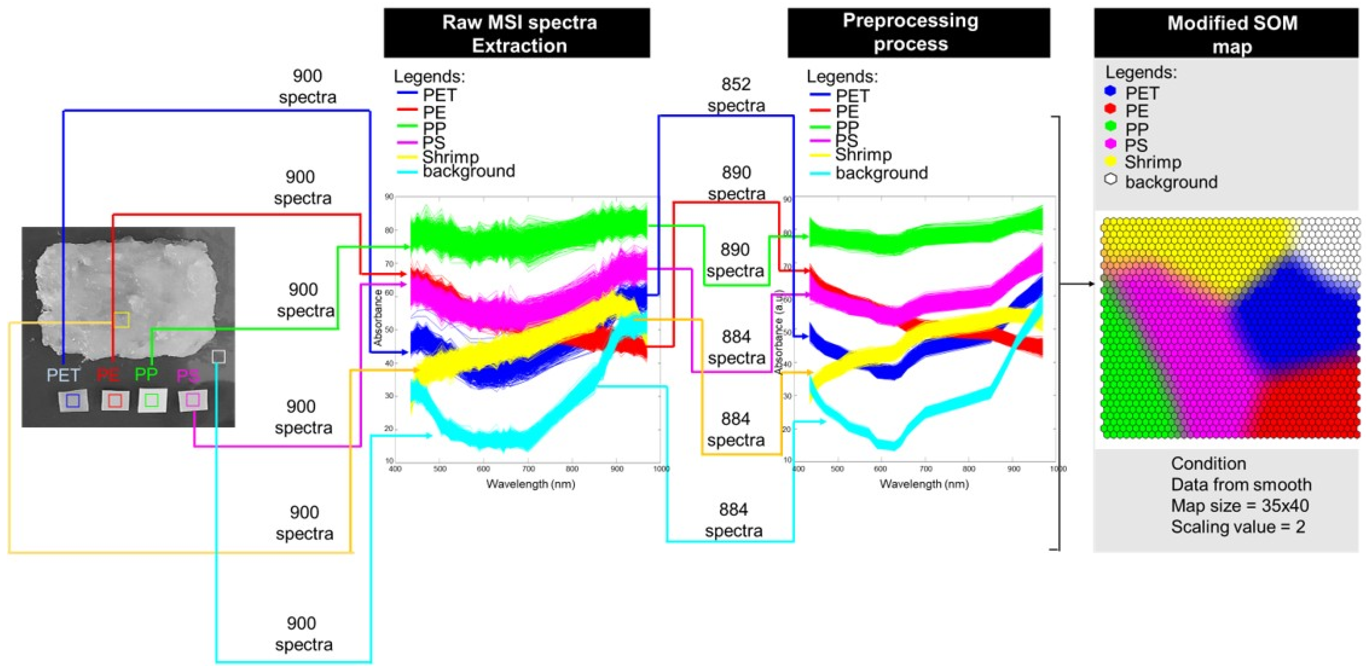
High-resolution images of minced shrimp samples with varying levels of MP contamination were captured using a VideometerLab2^® (Videometer A/S, Herlev, Denmark). This system includes a multispectral camera (Point Gray Research, Scorpion SCOR-20SOM, 1200 × 1200 pixels) that can capture 17 spectral images covering the visible to near-infrared (vis-NIR) range, from 435 to 970 nm. Before acquiring images, the instrument’s ‘auto light’ function was used to adjust the strobing duration of the LEDs, ensuring consistent illumination. Calibration included capturing images of three plates: a white plate for reference calibration, a dark plate for background correction, and a dotted plate for geometric alignment.

During the imaging process, the calibration set and prediction set were placed under controlled conditions in a dark chamber. A hollow sphere containing the camera was positioned above the sample platform to create a stable dark environment. Each sample was illuminated sequentially by 17 LEDs, generating a data cube that represented the spectral information for each LED.

2.4. Preprocessing

In this study, two sections are considered: the reference sample for constructing the supervised SOM (global SOM) and the calibration and prediction samples analyzed using this global SOM.

Regarding the reference samples used for the SOM constructed to classify and predict MP contamination in minced shrimp (calibration set and prediction set), these reference samples consisted of PET, PE, PP, PS, minced shrimp, and a background (with a blue substrate in this case). After capturing the reference samples with the MSI technique, we selected an image region as close as possible to the sample. This selection was performed to decrease the algorithm’s time calculation by focusing only on the essential region. Therefore, we obtained a single multispectral image with a spatial dimension of 500 × 380 pixels, as shown in the gray image in Figure 1. For each sample type—PET, PE, PP, PS, minced shrimp, and the background—we defined a region of interest (ROI) of 30 × 30 pixels. This resulted in 900 spectra (30 × 30 pixels) per sample, covering 17 wavelength bands ranging from 435 to 970 nm, allowing for a comprehensive spectral analysis of each sample. Each pixel corresponds to the physicochemical attributes of the segmented objects. These spectral data were used to construct the global SOM and were further used to classify MP types (qualitatively) and predict contamination levels in minced shrimp (quantitatively).

Before constructing the global SOM, preprocessing techniques are essential due to challenges with Vis-NIR multispectral imaging, such as noise from ambient light, electronic interference, and inconsistent lighting, which can distort spectral data. Additionally, sample characteristics like texture and moisture can affect reflections. These preprocessing steps improve data quality, reduce noise, and ensure effective analysis. The first step involved using the interquartile range (IQR) method, which demonstrates the difference between the 75th and the 25th percentiles [40]. It effectively addresses outliers and is reliable for identifying and removing sample pixels with erroneous measurements. The average MSI spectrum of each sample class was calculated as a centroid of the data class. Any sample with a Euclidean distance from the mean spectrum exceeding 1.5 times the IQR was considered an artifact and excluded from further analysis [39]. The following preprocessing step involved applying Savitzky–Golay smoothing (SGS) with a polynomial order of 2 and a smoothing points range of 11. This technique was used to reduce spectral differences and noise in the raw spectra of microplastics. The entire process of sample segmentation and preprocessing of the reference samples is illustrated in Figure 1.

As previously described, preprocessing techniques were applied after capturing the MSI image for the calibration and validation samples (Figures S1–S4). Each image considered the entire set of pixels from 300 × 500 pixels = 150,000 spectra. The spectral dimension spanned 17 wavelength bands, ranging from 435 to 970 nm, and none of the images involved selecting any region of interest or averaging the spectrum. We used a global SOM to analyze all of these images (see the right-hand side of Figures S1–S4).

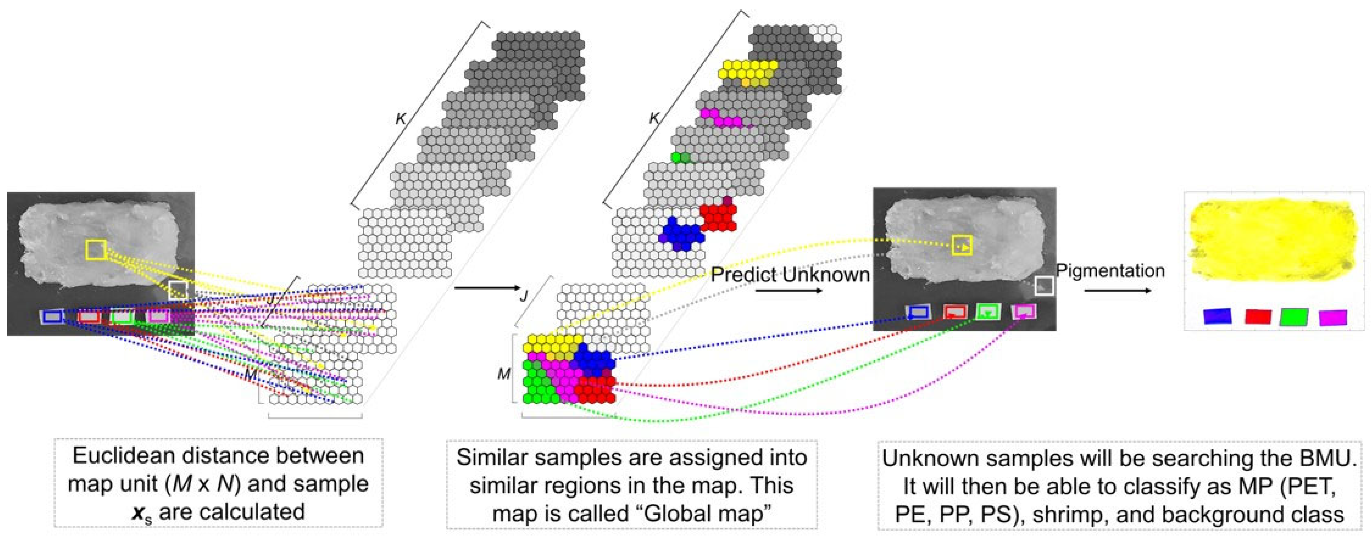
2.5. Modified Self-Organizing Map (SOM)

The MSI spectra of pure sample classes, including PET, PE, PP, PS, minced shrimp, and the background after performing preprocessing according to Section 2.4, were used as reference spectra to construct a global SOM. The overall process for creating the global SOM can be summarized in three steps: initialization of the weight vector, addition of a supervised class weight vector (scaling value) to differentiate between sample groups, and the training process to identify the best matching unit (BMU).

During the training phase, the SOM utilized reference spectral data, incorporating class labels (scaling values) to guide the formation of the map and enhance classification accuracy. The training process involved running multiple iterations—typically at least 10,000 times—to stabilize the map and fine-tune critical parameters such as the learning rate and the neighborhood function [41]. As the SOM learned the data, it organized them so that similar classes, which shared comparable chemical information, were mapped to nearby locations. Once the training was complete, a global SOM was generated, serving as a reference for classifying and predicting unknown samples. This map visually represents the relationships between different classes, with similar classes clustered together and assigned specific color tones based on their spectral similarities. The global SOM is illustrated in the modified SOM step in Figure 1.

After constructing the global SOM, which effectively organizes and represents the spectral data of known classes, the next step involved utilizing this global SOM to classify unknown MSI data based on their spectral characteristics. The spectral data from an unknown MP sample were projected onto the trained SOM (global SOM). This process involved mapping each pixel from the spectral image onto the global SOM and identifying the best matching unit (BMU) by calculating the smallest Euclidean distance (a measure of similarity) between the unknown sample’s spectrum and the reference spectra using Equations (1) and (2).

$$s({\mathit{x}}_o,{\mathit{w}}_g)=\sqrt{{\sum }_{j=1}^J{(x_{oj}-w_{gj})}^2}=\min \{s({\mathit{x}}_o,{\mathit{w}}_g)\},$$

(1)

k = argmin{s(x_o,w_g)},

(2)

where x_o is defined as the spectral pixel of the object, w_g is the weight vector on the global SOM most similar to x_o, and k denotes the map unit with the smallest Euclidean distance [39].

After identifying the best matching map unit, its color vector, comprising the R, G, and B values, was extracted and projected to the corresponding pixel. The process was repeated until the pixels on the object image were completely projected by the RGB value. These color patterns serve as visual markers for classifying each member of the class. For example, if the color pattern corresponded to PET, the sample was classified as PET; if it corresponded to PE, it was classified as PE, and so on. This enabled the classification of unknown samples based on distinct color shades corresponding to different classes. The classification of unknown samples is depicted in Figure 2. For a more detailed explanation of the SOM algorithm, refer to the earlier work by [39].

2.6. Evaluation of the SOM Model Performance

2.6.1. Qualitative Method

In this qualitative analysis, we aimed to evaluate the effectiveness of our model in classifying and identifying four types of microplastics (MPs) within the size range of 1 to 4 mm when placed on minced shrimp and shrimp shells. The four types of MPs—PET, PE, PP, and PS—were combined in a single image to determine whether our model could accurately classify and identify all four types simultaneously. To qualitatively assess the model’s performance, we employed color indices (red, green, and blue values) of the sample image. Each type of MP was assigned a specific color representation: PET was designated blue, PE red, PP green, and PS magenta. By analyzing the color distribution in the captured images, we could visually evaluate the model’s ability to distinguish between the different types of MPs and the shrimp samples. This method allowed us to determine the model’s effectiveness in accurately classifying the microplastics based on their unique spectral signatures and color profiles.

2.6.2. Quantitative Method

After color mapping, an automated counting process was employed for quantitative analysis. This method involves recording and counting color-coded pixels in the object images of the calibration set and prediction set, as mentioned in Section 2.2.2 above. By calculating the proportion of pixels associated with each MP type relative to the corresponding reference pixel count, researchers can derive a ratio correlated with the concentration of each MP type.

For example, consider PET at a concentration of 0.04% w/w, represented by blue pixels. First, the number of blue pixels in the reference set (on the left side of Figure S1) was counted, and this count was assumed to represent 100% PET. Next, the contaminated minced shrimp (on the right side of Figure S1) was analyzed to count the predicted PET blue pixels. To calculate the predicted percentage of PET, the number of predicted PET pixels was divided by the number of reference PET pixels, and the result was multiplied by 100. This process was also applied to other PET concentrations (e.g., 0.08%, 0.12%, 0.16%, 0.2%, 0.4%, 0.6%, 0.8%, and 1% w/w). The predicted concentrations were then plotted against the actual concentrations, and the coefficient of determination (R²) was used to evaluate model performance [42]. A higher R² indicated a stronger linear relationship and better model accuracy. The calculation formulas for R² are shown in Equation (3).

$${\mathrm{R}}^2 ={\displaystyle \frac{1-\sum _n^{i=1}( y_t^i-y^i) }{\sum _n^{i=1}( y_{t }^i-\overline{y}) }}$$

(3)

where R² represents the coefficient of determination, $y_t^i$ represents the predicted output, $y^i$ denotes the actual output, and $\overline{y}$ represents the mean of the predicted values across the n data points.

The same protocol was used for the other MPs (PE, PP, and PS), but each had a different designated color, i.e., red for PE, green for PP, and magenta for PS, as specified in the model algorithm. This approach offers valuable insights into the contamination levels of the MPs in the sample and assesses the quantitative accuracy of the SOM model.

2.7. Evaluation of the Size Limit Detection for Microplastics

The core idea of this approach is its capacity to classify MP particles by evaluating the proportional representation of pixels associated with the material in the imaging data rather than relying strictly on the physical size of the particles. This means that instead of solely measuring the dimensions of each MP piece, the method analyzes the distribution and abundance of relevant spectral pixels that correspond to the specific material. This is especially important because MPs exhibited considerable variation in size and shape. Traditional classification methods, which often depend on predefined physical dimensions, can encounter difficulties when dealing with smaller or irregularly shaped particles. By focusing on pixel-level data, this approach accommodates these variations and provides a more nuanced analysis of MP composition. It ensures that even small or fragmented particles with fewer representative pixels are still identified and classified accurately. This method enhances the reliability of MP detection and quantification, particularly in complex environmental samples where particles of different sizes coexist.

The classification process began by calculating the proportion of relevant pixels corresponding to each type of MP. The formula used for this calculation is presented in Equation (4).

$$\mathrm{Proportion} \mathrm{of} \mathrm{relevant} \mathrm{pixels}=\left({\displaystyle \frac{\mathrm{N}\mathrm{u}\mathrm{m}\mathrm{b}\mathrm{e}\mathrm{r} \mathrm{o}\mathrm{f} \mathrm{r}\mathrm{e}\mathrm{l}\mathrm{e}\mathrm{v}\mathrm{a}\mathrm{n}\mathrm{t} \mathrm{p}\mathrm{i}\mathrm{x}\mathrm{e}\mathrm{l}\mathrm{s}\left(\mathrm{M}\mathrm{P}\mathrm{s}\right)}{\mathrm{T}\mathrm{o}\mathrm{t}\mathrm{a}\mathrm{l} \mathrm{n}\mathrm{u}\mathrm{m}\mathrm{b}\mathrm{e}\mathrm{r} \mathrm{o}\mathrm{f} \mathrm{M}\mathrm{P} \mathrm{p}\mathrm{i}\mathrm{x}\mathrm{e}\mathrm{l}}}\right) \times 100$$

(4)

This formula allows researchers to quantify how much of the image is represented by a specific type of MP. For instance, in the example provided, four pieces of PET were analyzed, each with different sizes (4 mm, 3 mm, 2 mm, and 1 mm).. The classification relied on counting the number of pixels corresponding to the blue color index associated with PET, as determined by the BMU in the SOMs.

To evaluate whether each piece would be classified as PET, the number of blue pixels was counted and compared to the total number of pixels representing all MP types (indicated by other colors such as red, green, and magenta). The proportion of blue pixels was calculated using the formula in Equation (5).

$$\mathrm{Proportion} \mathrm{of} \mathrm{blue} \mathrm{pixels}=\left({\displaystyle \frac{\mathrm{N}\mathrm{u}\mathrm{m}\mathrm{b}\mathrm{e}\mathrm{r} \mathrm{o}\mathrm{f} \mathrm{b}\mathrm{l}\mathrm{u}\mathrm{e} \mathrm{p}\mathrm{i}\mathrm{x}\mathrm{e}\mathrm{l}\mathrm{s}\left(\mathrm{M}\mathrm{P}\mathrm{s}\right)}{\mathrm{T}\mathrm{o}\mathrm{t}\mathrm{a}\mathrm{l} \mathrm{n}\mathrm{u}\mathrm{m}\mathrm{b}\mathrm{e}\mathrm{r} \mathrm{o}\mathrm{f} \mathrm{M}\mathrm{P} \mathrm{p}\mathrm{i}\mathrm{x}\mathrm{e}\mathrm{l}}}\right)$$

(5)

A critical aspect of this classification method is the establishment of a cutoff percentage. In this study, a cutoff of 25% was deemed acceptable for classification. This threshold is significant because it reflects an equal distribution of pixels among the four MP types being analyzed. Setting this cutoff ensures that only pieces with substantial relevant pixel representation are classified into a specific type, aligning with theoretical expectations regarding the distribution of MPs and providing a reasonable baseline for classification.

The same principle applied to other MPs: PE, PP, and PS. Their relevant pixel proportions, assigned red, green, and magenta in the SOM model, were calculated using Equations (6)–(8).

$$\mathrm{Proportion} \mathrm{of} \mathrm{red} \mathrm{pixels}=\left({\displaystyle \frac{\mathrm{N}\mathrm{u}\mathrm{m}\mathrm{b}\mathrm{e}\mathrm{r} \mathrm{o}\mathrm{f} \mathrm{r}\mathrm{e}\mathrm{d} \mathrm{p}\mathrm{i}\mathrm{x}\mathrm{e}\mathrm{l}\mathrm{s}\left(\mathrm{M}\mathrm{P}\mathrm{s}\right)}{\mathrm{T}\mathrm{o}\mathrm{t}\mathrm{a}\mathrm{l} \mathrm{n}\mathrm{u}\mathrm{m}\mathrm{b}\mathrm{e}\mathrm{r} \mathrm{o}\mathrm{f} \mathrm{M}\mathrm{P} \mathrm{p}\mathrm{i}\mathrm{x}\mathrm{e}\mathrm{l}}}\right) \times 100$$

(6)

$$\mathrm{Proportion} \mathrm{of} \mathrm{green} \mathrm{pixels}=\left({\displaystyle \frac{\mathrm{N}\mathrm{u}\mathrm{m}\mathrm{b}\mathrm{e}\mathrm{r} \mathrm{o}\mathrm{f} \mathrm{g}\mathrm{r}\mathrm{e}\mathrm{e}\mathrm{n} \mathrm{p}\mathrm{i}\mathrm{x}\mathrm{e}\mathrm{l}\mathrm{s} \left(\mathrm{M}\mathrm{P}\mathrm{s}\right)}{\mathrm{T}\mathrm{o}\mathrm{t}\mathrm{a}\mathrm{l} \mathrm{n}\mathrm{u}\mathrm{m}\mathrm{b}\mathrm{e}\mathrm{r} \mathrm{o}\mathrm{f} \mathrm{M}\mathrm{P} \mathrm{p}\mathrm{i}\mathrm{x}\mathrm{e}\mathrm{l}}}\right) \times 100$$

(7)

$$\mathrm{Proportion} \mathrm{of} \mathrm{magenta} \mathrm{pixels}=\left({\displaystyle \frac{\mathrm{N}\mathrm{u}\mathrm{m}\mathrm{b}\mathrm{e}\mathrm{r} \mathrm{o}\mathrm{f} \mathrm{m}\mathrm{a}\mathrm{g}\mathrm{e}\mathrm{n}\mathrm{t}\mathrm{a} \mathrm{p}\mathrm{i}\mathrm{x}\mathrm{e}\mathrm{l}\mathrm{s}\left(\mathrm{M}\mathrm{P}\mathrm{s}\right)}{\mathrm{T}\mathrm{o}\mathrm{t}\mathrm{a}\mathrm{l} \mathrm{n}\mathrm{u}\mathrm{m}\mathrm{b}\mathrm{e}\mathrm{r} \mathrm{o}\mathrm{f} \mathrm{M}\mathrm{P} \mathrm{p}\mathrm{i}\mathrm{x}\mathrm{e}\mathrm{l}}}\right) \times 100$$

(8)

2.8. Principal Component Analysis (PCA)

Principal component analysis (PCA) is a widely used technique for analyzing multivariate data, such as signals, spectral data, physicochemical properties, and multispectral images. It is particularly effective for high-dimensional datasets, as it uncovers hidden patterns and simplifies complex information [43,44]. PCA is typically used for exploratory purposes to reduce data size by projecting samples into a smaller subspace. In this subspace, the axes, known as principal components (PCs), are linear combinations of the original variables calculated to represent the maximum variance. PCA enables the visualization of how samples are distributed over time in score plots, facilitating the exploration of relationships between individual measurements or observations, such as identifying trends, groups, extreme objects, and more [43,44,45,46].

In this study, PCA was applied to analyze MSI images of MPs and shrimp, comparing its effectiveness with the SOM model. The PC1 score, representing the primary component, was plotted as a contour map to highlight spectral variance and facilitate different types of samples [47] such as MPs and shrimp components.

All computational procedures were conducted using MATLAB R2022a (The MathWorks, Natick, MA, USA) with an in-house coding algorithm.

3. Results and Discussion

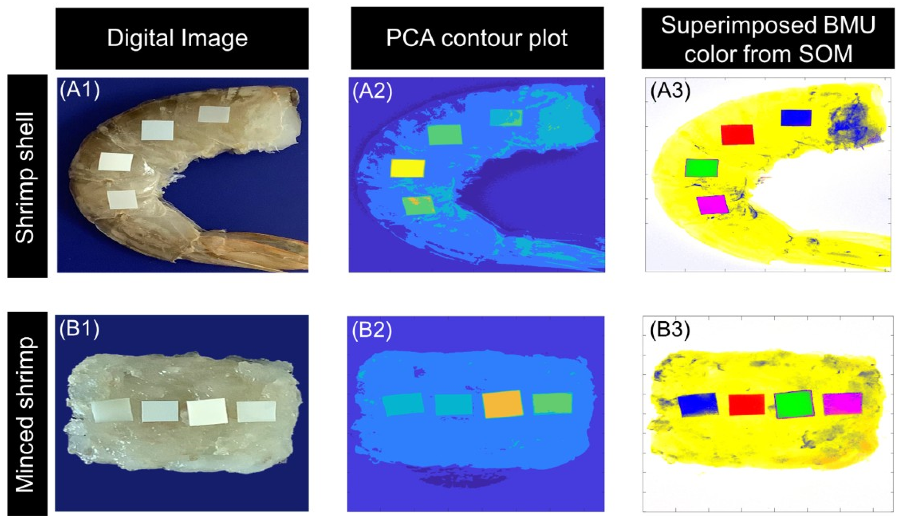
3.1. Qualitative Analysis

The current study shows the feasibility and effectiveness of a modified supervised SOM combined with Vis-NIR MSI for the rapid qualitative and quantitative analysis of microplastic contamination in seafood, particularly shrimp. Our results demonstrate that the SOM method facilitated clear visual discrimination of four common MP types—PET, PE, PP, and PS—even within complex biological matrices such as minced shrimp and shrimp shells.

For qualitative analysis, we focused on visualizing and interpreting the data to assess the model’s ability to classify and identify different types of MPs present in shrimp samples. As shown in Figure 3, it consists of a digital image, the PCA (PC1) contour plot, and the superimposed BMU map generated by the SOM algorithm for shrimp shell and minced shrimp. In our model, each type of MP—PET, PE, PP, and PS— as well as shrimp and background are assigned blue, red, green, magenta, yellow, and white colors, respectively. For effective qualitative assessment, the sample should display these assigned colors consistently, reflecting correct classification based on spectral characteristics.

The results in Figure 3A3,B3 demonstrate that the superimposed BMU color maps from global SOMs successfully enabled a clear visual differentiation of the four MP types, shrimp tissue, and background. This consistent color assignment highlights the model’s capability to accurately distinguish between different materials based on their spectral profiles, confirming its utility for qualitative analysis. The appearance of PET-labeled pixels in shrimp tissue may result from spectral overlap or PET’s partial transparency, influenced by factors like lighting, sample thickness, and RGB mapping. While overall classification remains unaffected, further research is needed to understand how such factors impact SOM accuracy and color representation. In contrast, the PCA contour plot and digital image could not effectively classify any unknown MP contamination in either shrimp shell or minced shrimp. One possible reason for this discrepancy is that PCA depends on linear relationships [48], while SOMs, as neural networks, are capable of capturing both linear and nonlinear patterns within the data [33,49]. This ability of SOMs is particularly beneficial when detecting MP contamination in biological samples (such as shrimp), as the interactions between MPs and shrimp produce complex spectral data. Furthermore, the use of supervised SOMs enables the incorporation of class information during training, thereby improving classification accuracy. In contrast, PCA operates in an unsupervised manner without utilizing class labels. Although we focused on PC1 in the main figures for clarity, the additional principal components (PC2–PC6) are shown in Figure S5 to illustrate their contribution to the separation of microplastic types. This additional information provides a broader context for understanding PCA’s limitations and comparative performance. This statement is supported by Makmuang et al. (2021) [41], who demonstrated that SOMs outperform PCA in classifying weedy and cultivated rice, providing clearer clustering and less overlap among sample groups. Similarly, Makmuang et al. (2024) [40] reported that supervised SOMs outperformed PCA in classifying Thai melon seeds, offering superior separation of sample clusters and improving classification performance.

The ability to visually identify and differentiate microplastics underscores the effectiveness of advanced analytical techniques such as multispectral imaging combined with SOMs, which capture unique spectral signatures for various polymer types. This not only aids in MP classification but also enhances our understanding of their sources, pathways, and ecological impacts. Compared to conventional methods such as PCA, the modified SOM offers superior specificity in classifying MP types. While PCA is useful for visualizing data patterns, it lacks the detailed classification capabilities of SOM, making it a more robust tool for environmental monitoring and microplastic analysis.

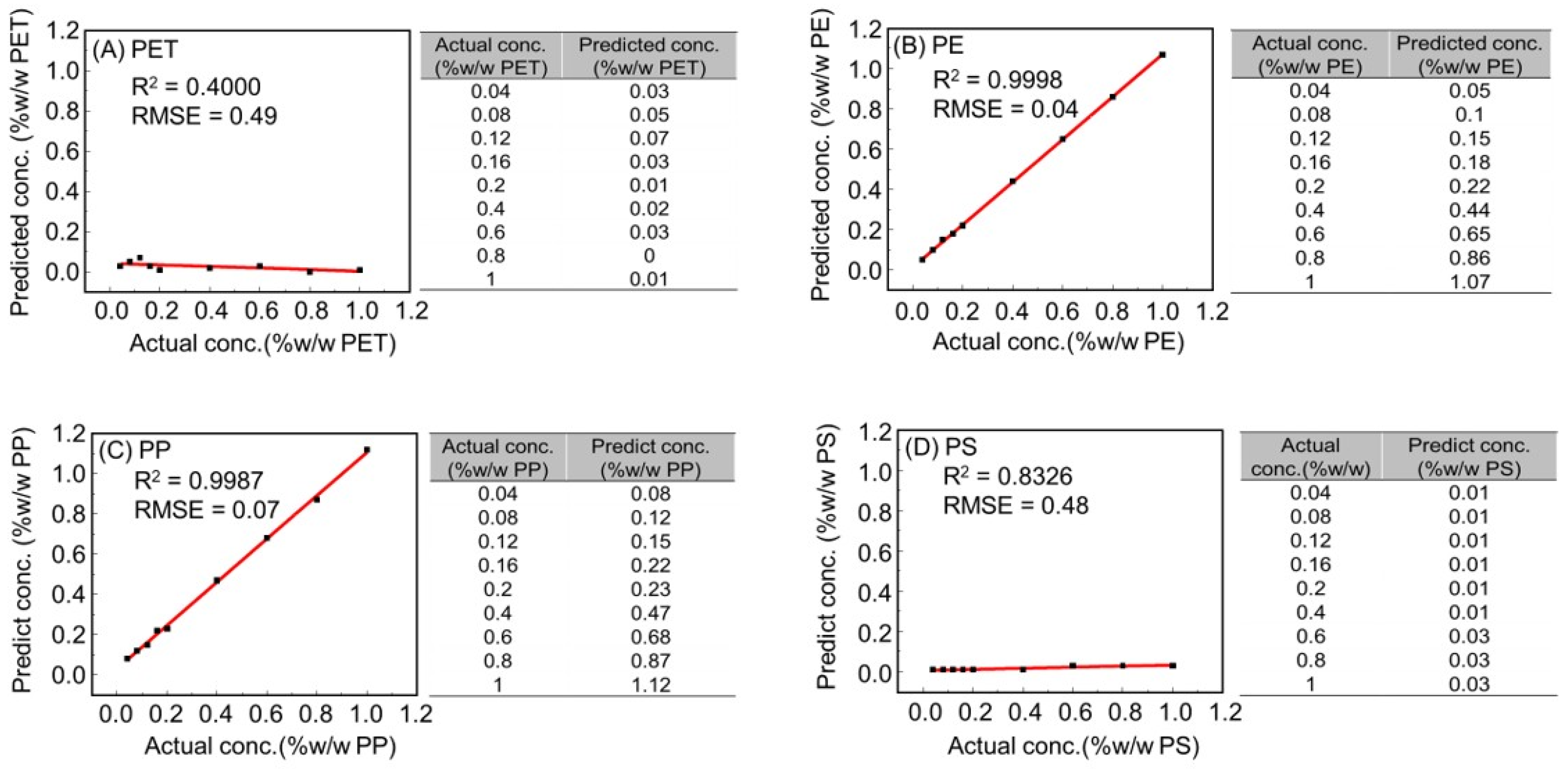
3.2. Quantitative Analysis

Qualitative analysis demonstrated the effectiveness of SOMs in classifying the four types of MP contamination—PET, PE, PP, and PS—found in minced shrimp and shrimp samples. This classification was accomplished by projecting RGB values onto the pixels of object images, which allowed for a clear visual identification and assessment of the distribution of contamination. However, qualitative analysis alone was insufficient to achieve the ultimate goals of this work; therefore, quantitative analysis was implemented. The quantitative analysis of microplastic contamination in minced shrimp using the global SOM model revealed varying levels of prediction accuracy across different polymers, as indicated by the R² values. Figures S1–S4 illustrate the superimposed map on the right-hand side, showing the color index of the BMUs from the global SOM based on spectral data for PET, PE, PP, and PS mixtures at concentrations ranging from 0.04% to 1% w/w. An inset table displays MP concentration calculations using pixel counting based on the BMU color index from the SOMs. Additionally, the pixel counting of the reference set (calibration set) and the predicted set were plotted against each other to compare the actual concentrations with the predicted concentrations, with the R² values used to evaluate model performance, as shown in Figure 4. The methodology for calculating the % actual concentration and prediction based on the pixels in the object is detailed in Section 2.6.2.

The results presented in Figure 4 highlight the varying predictive performance of different microplastic types using the SOM model. Notably, the PET mixture had the lowest R² value of 0.40, suggesting significant difficulties in accurately predicting its concentration. The inverse relationship between the predicted and actual values suggests that the SOM model struggles with PET, resulting in highly inaccurate predictions. The possible reason may be attributed to the intrinsic properties of PET, which provide a transparent nature and weak absorption in the Vis-NIR range, resulting in subtle spectral features that lead to a low signal-to-noise ratio, making it difficult for the imaging system to generate distinct and reliable spectral signatures. This can interfere with the model’s ability to effectively analyze and classify the spectral data [50,51,52].

In contrast, the PS mixture demonstrated a moderate prediction accuracy, with an R² value of 0.83 (Figure 4D). However, the predicted number of object pixels (from the prediction set) did not align well with the actual pixel count (from the calibration set), likely suggesting difficulty in accurately estimating PS concentrations. This is consistent with the expectations for PET results discussed earlier. A possible explanation involves the structural properties of PET and PS, which contain functional groups that interact more readily with organic materials compared to other MPs. This observation aligns with studies indicating that PS and PET can interact with organic proteins. For example, Krishna de Guzman et al. (2023) [53] demonstrated that pepsin interacts with PS MP, resulting in structural changes to pepsin, inhibited activity, and reduced digestibility. Similarly, Gligorijevic et al. (2024) [54] found that ovalbumin also interacts with PS and PET microplastics.

In contrast, the PE mixture achieved an exceptional R² value of 0.99, the highest among all analyzed MPs (Figure 4B). This high accuracy can likely be attributed to the non-transparent nature of PE, which allows for the effective mapping of objects in the images without interference from light scattering during spectral readings. PE showed superior prediction performance (R² ≈ 0.99), possibly due to its simpler, non-polar structure and consistent optical properties, which may lead to clearer and more stable spectral responses. While PET and PS possess aromatic groups that can enhance light absorption, their interactions with the biological matrix—such as shrimp proteins and water—might introduce spectral complexity that affects prediction accuracy. This is supported by our previous work [27], where partial least squares discriminant analysis (PLS-DA) showed moderate effectiveness, and MSI demonstrated good sensitivity for PE, confirming its viability for MP analysis.

Similar to polypropylene (PP) also showed strong performance, with an R² value of 0.99 (Figure 4C). The predictions for PP concentrations closely aligned with the actual values, indicating that the SOM model is effective in predicting this type of MP. The high R² can be attributed to the distinct spectral characteristics of PP, which allow for reliable differentiation from other polymers.

By calculating the proportion of pixels associated with each MP type relative to the total number of pixels in the image, researchers can derive a ratio that correlates with the concentration of each MP type. This quantitative assessment provides valuable insights into the MP pollution levels present in the analyzed environmental samples.

It is worth noting that using a global SOM for classification in this context allows for the full analysis of the entire MSI image rather than relying on average values or ROI. This approach aligns with the findings of Makmuang et al. (2023) [39], who also utilized SOM to predict weedy rice and reported that analyzing the entire image yielded better performance than the methods focused on specific ROIs or average spectra. However, in the current study, the performance of models used to detect and quantify MPs appeared to depend on the type of MP being analyzed. The results highlight the varying effectiveness of the SOM model in predicting different types of MPs. While PE and PP demonstrated high prediction accuracy, PET and PS proved to be significantly more challenging and require further investigation. The overall results suggest that the SOM, combined with Vis-NIR MSI, eliminates the need for pre-sorting or chemical treatments and offers an accurate, rapid, and interpretable method for classifying various polymer types in complex food matrices, with strong potential for application in large-scale environmental and food safety monitoring. However, prediction performance still varies depending on the type of MP being analyzed. Understanding these discrepancies is crucial for improving the model’s performance and enhancing the reliability of MP quantification in environmental samples. Future work may focus on refining the analytical techniques and addressing the limitations associated with transparent plastics while also investigating the underlying chemical mechanisms—such as polymer–protein and polymer–water interactions—that may influence spectral behavior, to achieve more consistent and accurate predictions across all MP types.

3.3. Size-Based Analysis

The global SOM projection has proven to be an effective tool for classifying different types of MP, such as PET, PE, PP, and PS, based on their spectral signatures derived from MSI data. The strength of the SOM method lies in its ability to analyze the spectral characteristics of the MPs independently of their physical size. This means that even if the particles vary in size within the 1$–$4 mm range, the SOM can accurately classify them based on their unique spectral profiles, enhancing the robustness of the classification process and allowing for the reliable identification of MPs in complex environmental matrices. To support this assertion, this section focuses on determining the minimum size of MPs that our system can classify, specifically targeting larger MPs within the 1−4 mm range. This size is significant due to its frequent occurrence in environmental samples and its potential for ingestion by marine and terrestrial organisms, which can result in physical harm, toxic effects, and bioaccumulation in the food chain.

The individual MPs of 1, 2, 3, and 4 mm on shrimp shells as illustrated in the digital images of Figure 5A1, Figure 5B1, Figure 5C1, and Figure 5D1 for PET, PE, PP, and PS, respectively. As shown in Figure 5A3–D3, SOM accurately classified all MPs. In the PET case shown in Figure 5A3, any microplastic piece with a proportion of blue pixels exceeding 25% was classified as PET. The results show that all four PET pieces had a blue pixel proportion greater than 84%. This high percentage confirmed a strong representation of PET in the image, demonstrating that all pieces were accurately classified as PET.

The same results are similar to those of other MP types, including PE, PP, and PS, as illustrated in Figure 5B3, Figure 5C3, and Figure 5D3, respectively. The proportion of relevant pixels corresponding to their assigned colors in the SOM model was different: red for PE, green for PP, and magenta for PS. The results show that for each MP type—PE (Figure 5B3), PP (Figure 5C3), and PS (Figure 5D3)—all particle sizes (1, 2, 3, and 4 mm) had a proportion of relevant pixels exceeding 25%. This indicates accurate classification into their respective class, suggesting that the modified SOM method is highly effective in classifying microplastic particles, including smaller ones as small as 1 mm. Furthermore, it outperformed PCA (PC1 contour plot), as evidenced in Figure 5A2–D2. This capability is particularly valuable for environmental monitoring and assessment, as it provides a more detailed understanding of microplastic distribution and its potential ecological impacts.

The approach of counting RGB pixels is particularly advantageous as it addresses the limitations associated with conventional methods that may struggle with the diverse types, shapes, and sizes of MPs. By focusing on pixel counts, this methodology offers a comprehensive assessment of microplastic presence, enabling more accurate monitoring and evaluation of MP pollution. The research shows that advanced imaging technologies and machine learning could be used to detect microplastic contamination in seafood products. Furthermore, this study demonstrates that the minimum MP particle size classified by our SOM is 1 mm. However, there is also potential for the SOM to classify and analyze smaller particles. This approach evaluates MPs on a pixel-by-pixel basis, which means its effectiveness largely depends on the resolution of the imaging technique used. The comparison based on literature references to highlight the advantages of our approach is presented in the Supporting Information, Table S1.

It is worth noting that while our current study focuses on regular MP shapes, the pixel-level analysis enables the possibility of classifying irregularly shaped MPs, as evidenced by our previous research involving weedy rice, which featured naturally irregular shapes [39]. Similarly, Lorenzo-Navarro et al. [55] developed an automated method using deep learning to count and classify irregularly shaped MPs, achieving an impressive average classification accuracy of 98.11%. Building on this foundation, future studies will aim to evaluate the performance of our method on a wider range of microplastics—particularly those with more complex and irregular geometries—as well as across various shrimp species. Furthermore, in the future, it may be possible to apply this method to microplastics smaller than 1 mm if high-resolution MSI is employed. This would enable the SOM to detect particles as small as the resolution of the imaging machine allows.

4. Conclusions

The results presented in this study establish a proof of concept for applying the Vis-NIR multispectral imaging (MSI) system to identify and predict microplastic (MP) particles (PET, PE, PP, and PS) in the size range of 1–4 mm directly within minced shrimp contamination scenarios, without extensive sample preparation. This approach enables the rapid qualitative and quantitative assessment of MP contamination. In qualitative analysis, the SOM provided clearer visual identification and distinction among the four MP types compared to PCA, offering superior insights into the types and distribution of MPs within the samples. For quantitative analysis, the modified SOM achieved a high R² > 0.99 for PE and PP, indicating a strong correlation between predicted and actual MP concentrations. This demonstrates the model’s ability to accurately predict MP concentrations in shrimp samples. Crucially, this method eliminates the need for manual sorting of particles, significantly reducing analysis time, sample handling, and the risk of particle loss or disruption. The integration of advanced imaging and machine learning significantly improves microplastic detection, enabling efficient large-scale monitoring in complex biological samples. Despite the promising results, several limitations persist. The accuracy of the predictions varied by plastic type; for instance, PET showed lower accuracy due to its transparency. While the current method is effective for detecting particles larger than 1 mm, advancements in imaging technology are necessary to identify smaller microplastics. It is also important to extend this method to include other seafood species and a wider range of microplastic types in order to assess its general applicability. The method should also be extended to other seafood species and a broader range of microplastic types to evaluate its generalizability. Another limitation of this research is that the quantitative results obtained with the modified SOMs were not compared with other machine learning techniques. Future studies will address this gap by evaluating and benchmarking the model’s performance against alternative algorithms. Additionally, applying this method to real-world samples, such as shrimp meat and intestines, will be crucial for enhancing its practical relevance and improving food safety, thereby protecting consumer health.

References

1. Marchesi, C.; Rani, M.; Federici, S.; Alessandri, I.; Vassalini, I.; Ducoli, S.; Borgese, L.; Zacco, A.; Núñez-Delgado, A.; Bontempi, E.; et al. Quantification of Ternary Microplastic Mixtures through an Ultra-Compact Near-Infrared Spectrometer Coupled with Chemometric Tools. Environ. Res. 2023, 216, 114632. [Google Scholar] [CrossRef] [PubMed]
2. Perumpully, S.J.; Kumar, R.P.; Gautam, S.; Ambade, B.; Gautam, A.S. An Inclusive Trend Study of Evaluation and Scientometric Analysis of Microplastics. Phys. Chem. Earth Parts A/B/C 2023, 132, 103455. [Google Scholar] [CrossRef]
3. Sravya, G.C.; Gautam, S.; Kumar, K.U.; Poonguzhali, R.S.; Manuel, R.I. Assessing LDPE Microplastics’ Impact on Green Gram (Vigna radiata L. Wilczek) Cultivation: A Greenhouse Pot Experiment. Phys. Chem. Earth Parts A/B/C 2024, 136, 103710. [Google Scholar] [CrossRef]
4. Khan, M.B.; Urmy, S.Y.; Setu, S.; Kanta, A.H.; Gautam, S.; Eti, S.A.; Rahman, M.M.; Sultana, N.; Mahmud, S.; Baten, M.A. Abundance, Distribution and Composition of Microplastics in Sediment and Fish Species from an Urban River of Bangladesh. Sci. Total Environ. 2023, 885, 163876. [Google Scholar] [CrossRef]
5. United Nations Environment Assembly. Plastic Waste Causes Financial Damage of US$13 Billion to Marine Ecosystems Each Year as Concern Grows over Microplastics. Available online: https://www.unep.org/news-and-stories/press-release/plastic-waste-causes-financial-damage-us13-billion-marine-ecosystems (accessed on 15 June 2025).
6. Ogunola, O.S.; Onada, O.A.; Falaye, A.E. Mitigation Measures to Avert the Impacts of Plastics and Microplastics in the Marine Environment (A Review). Environ. Sci. Pollut. Res. 2018, 25, 9293–9310. [Google Scholar] [CrossRef]
7. Mouat, J.; Lozano, R.L.; Bateson, H. Economic Impacts of Marine Litter; KIMO: Shetland, UK, 2010. [Google Scholar]
8. Meng, X.; Chen, S.; Li, D.; Song, Y.; Sun, L. Identification of Marine Microplastics Based on Laser-Induced Fluorescence and Principal Component Analysis. J. Hazard. Mater. 2024, 465, 133352. [Google Scholar] [CrossRef]
9. Jin, N.; Song, Y.; Ma, R.; Li, J.; Li, G.; Zhang, D. Characterization and Identification of Microplastics Using Raman Spectroscopy Coupled with Multivariate Analysis. Anal. Chim. Acta 2022, 1197, 339519. [Google Scholar] [CrossRef]
10. Adeogun, A.O.; Ibor, O.R.; Khan, E.A.; Chukwuka, A.V.; Omogbemi, E.D.; Arukwe, A. Detection and Occurrence of Microplastics in the Stomach of Commercial Fish Species from a Municipal Water Supply Lake in Southwestern Nigeria. Environ. Sci. Pollut. Res. 2020, 27, 31035–31045. [Google Scholar] [CrossRef]
11. Ding, J.; Zhang, S.; Razanajatovo, R.M.; Zou, H.; Zhu, W. Accumulation, Tissue Distribution, and Biochemical Effects of Polystyrene Microplastics in the Freshwater Fish Red Tilapia (Oreochromis niloticus). Environ. Pollut. 2018, 238, 1–9. [Google Scholar] [CrossRef]
12. Catarino, A.I.; Macchia, V.; Sanderson, W.G.; Thompson, R.C.; Henry, T.B. Low Levels of Microplastics (MP) in Wild Mussels Indicate That MP Ingestion by Humans Is Minimal Compared to Exposure via Household Fibres Fallout during a Meal. Environ. Pollut. 2018, 237, 675–684. [Google Scholar] [CrossRef]
13. Li, J.Y.Q.; Nankervis, L.; Dawson, A.L. Digesting the Indigestible: Microplastic Extraction from Prawn Digestive Tracts. Front. Environ. Chem. 2022, 3, 903314. [Google Scholar] [CrossRef]
14. My, T.T.A.; Dat, N.D.; Hung, N.Q. Occurrence and Characteristics of Microplastics in Wild and Farmed Shrimps Collected from Cau Hai Lagoon, Central Vietnam. Molecules 2023, 28, 4634. [Google Scholar] [CrossRef]
15. Gurjar, U.R.; Xavier, M.; Nayak, B.B.; Ramteke, K.; Deshmukhe, G.; Jaiswar, A.K.; Shukla, S.P. Microplastics in Shrimps: A Study from the Trawling Grounds of North Eastern Part of Arabian Sea. Environ. Sci. Pollut. Res. 2021, 28, 48494–48504. [Google Scholar] [CrossRef]
16. Niemcharoen, S.; Haetrakul, T.; Palić, D.; Chansue, N. Microplastic-Contaminated Feed Interferes with Antioxidant Enzyme and Lysozyme Gene Expression of Pacific White Shrimp (Litopenaeus vannamei) Leading to Hepatopancreas Damage and Increased Mortality. Animals 2022, 12, 3308. [Google Scholar] [CrossRef]
17. Hossain, M.S.; Rahman, M.S.; Uddin, M.N.; Sharifuzzaman, S.M.; Chowdhury, S.R.; Sarker, S.; Nawaz Chowdhury, M.S. Microplastic Contamination in Penaeid Shrimp from the Northern Bay of Bengal. Chemosphere 2020, 238, 124688. [Google Scholar] [CrossRef] [PubMed]
18. De-la-Torre, G.E. Microplastics: An Emerging Threat to Food Security and Human Health. J. Food Sci. Technol. 2020, 57, 1601–1608. [Google Scholar] [CrossRef]
19. Huang, H.; Qureshi, J.U.; Liu, S.; Sun, Z.; Zhang, C.; Wang, H. Hyperspectral Imaging as a Potential Online Detection Method of Microplastics. Bull. Environ. Contam. Toxicol. 2021, 107, 754–763. [Google Scholar] [CrossRef]
20. Gautam, S.; Rathikannu, S.; Katharine, S.P.; Marak, L.K.R.; Alshehri, M. Beyond the Surface: Microplastic Pollution Its Hidden Impact on Insects and Agriculture. Phys. Chem. Earth Parts A/B/C 2024, 135, 103663. [Google Scholar] [CrossRef]
21. Gebejes, A.; Hrovat, B.; Semenov, D.; Kanyathare, B.; Itkonen, T.; Keinänen, M.; Koistinen, A.; Peiponen, K.E.; Roussey, M. Hyperspectral Imaging for Identification of Irregular-Shaped Microplastics in Water. Sci. Total Environ. 2024, 944, 173811. [Google Scholar] [CrossRef]
22. de Jourdan, B.; Philibert, D.; Asnicar, D.; Davis, C.W. Microplastic Biomonitoring Studies in Aquatic Species: A Review & Quality Assessment Framework. Sci. Total Environ. 2024, 957, 177541. [Google Scholar] [CrossRef]
23. Marcuello, C. Present and Future Opportunities in the Use of Atomic Force Microscopy to Address the Physico-Chemical Properties of Aquatic Ecosystems at the Nanoscale Level. Int. Aquat. Res. 2022, 14, 231–240. [Google Scholar] [CrossRef]
24. Vidal, C.; Pasquini, C. A Comprehensive and Fast Microplastics Identification Based on Near-Infrared Hyperspectral Imaging (HSI-NIR) and Chemometrics. Environ. Pollut. 2021, 285, 117251. [Google Scholar] [CrossRef]
25. Piarulli, S.; Malegori, C.; Grasselli, F.; Airoldi, L.; Prati, S.; Mazzeo, R.; Sciutto, G.; Oliveri, P. An Effective Strategy for the Monitoring of Microplastics in Complex Aquatic Matrices: Exploiting the Potential of Near Infrared Hyperspectral Imaging (NIR-HSI). Chemosphere 2022, 286, 131861. [Google Scholar] [CrossRef] [PubMed]
26. Faltynkova, A.; Wagner, M. Developing and Testing a Workflow to Identify Microplastics Using Near Infrared Hyperspectral Imaging. Chemosphere 2023, 336, 139186. [Google Scholar] [CrossRef] [PubMed]
27. Makmuang, S.; Aït-Kaddour, A. Assessment of Microplastic Contamination in Shrimp Utilizing Multispectral Imaging, Fluorescence, and Infrared Spectroscopy. J. Food Compos. Anal. 2025, 146, 107864. [Google Scholar] [CrossRef]
28. Manley, M. Near-Infrared Spectroscopy and Hyperspectral Imaging: Non-Destructive Analysis of Biological Materials. Chem. Soc. Rev. 2014, 43, 8200–8214. [Google Scholar] [CrossRef]
29. Okere, E.E.; Ambaw, A.; Perold, W.J.; Opara, U.L. Vis-NIR and SWIR Hyperspectral Imaging Method to Detect Bruises in Pomegranate Fruit. Front. Plant Sci. 2023, 14, 1151697. [Google Scholar] [CrossRef]
30. Lanjewar, M.G.; Asolkar, S.; Parab, J.S.; Morajkar, P.P. Detecting Starch-Adulterated Turmeric Using Vis-NIR Spectroscopy and Multispectral Imaging with Machine Learning. J. Food Compos. Anal. 2024, 136, 106700. [Google Scholar] [CrossRef]
31. Kohonen, T. The Self-Organizing Map. Proc. IEEE 1990, 78, 1464–1480. [Google Scholar] [CrossRef]
32. Brereton, R.G. Self Organising Maps for Visualising and Modelling. Chem. Cent. J. 2012, 6, S1. [Google Scholar] [CrossRef]
33. Lloyd, G.R.; Wongravee, K.; Silwood, C.J.L.; Grootveld, M.; Brereton, R.G. Self Organising Maps for Variable Selection: Application to Human Saliva Analysed by Nuclear Magnetic Resonance Spectroscopy to Investigate the Effect of an Oral Healthcare Product. Chemom. Intell. Lab. Syst. 2009, 98, 149–161. [Google Scholar] [CrossRef]
34. Devriese, L.I.; van der Meulen, M.D.; Maes, T.; Bekaert, K.; Paul-Pont, I.; Frère, L.; Robbens, J.; Vethaak, A.D. Microplastic Contamination in Brown Shrimp (Crangon crangon, Linnaeus 1758) from Coastal Waters of the Southern North Sea and Channel Area. Mar. Pollut. Bull. 2015, 98, 179–187. [Google Scholar] [CrossRef]
35. Murray, F.; Cowie, P.R. Plastic Contamination in the Decapod Crustacean Nephrops norvegicus (Linnaeus, 1758). Mar. Pollut. Bull. 2011, 62, 1207–1217. [Google Scholar] [CrossRef]
36. Braid, H.E.; Deeds, J.; DeGrasse, S.L.; Wilson, J.J.; Osborne, J.; Hanner, R.H. Preying on Commercial Fisheries and Accumulating Paralytic Shellfish Toxins: A Dietary Analysis of Invasive Dosidicus gigas (Cephalopoda Ommastrephidae) Stranded in Pacific Canada. Mar. Biol. 2012, 159, 25–31. [Google Scholar] [CrossRef]
37. dos Anjos Guimarães, G.; de Moraes, B.R.; Ando, R.A.; Sant’Anna, B.S.; Perotti, G.F.; Hattori, G.Y. Microplastic Contamination in the Freshwater Shrimp Macrobrachium amazonicum in Itacoatiara, Amazonas, Brazil. Environ. Monit. Assess. 2023, 195, 434. [Google Scholar] [CrossRef]
38. Saha, G.; Saha, S.C. Tiny Particles, Big Problems: The Threat of Microplastics to Marine Life and Human Health. Processes 2024, 12, 1401. [Google Scholar] [CrossRef]
39. Makmuang, S.; Terdwongworakul, A.; Vilaivan, T.; Maher, S.; Ekgasit, S.; Wongravee, K. Mapping Hyperspectral NIR Images Using Supervised Self-Organizing Maps: Discrimination of Weedy Rice Seeds. Microchem. J. 2023, 190, 108599. [Google Scholar] [CrossRef]
40. Makmuang, S.; Vilaivan, T.; Maher, S.; Ekgasit, S.; Wongravee, K. Discrimination of Thai Melon Seeds Using Near-Infrared Spectroscopy and Adaptive Self-Organizing Maps. Chemom. Intell. Lab. Syst. 2024, 245, 105060. [Google Scholar] [CrossRef]
41. Makmuang, S.; Nootchanat, S.; Ekgasit, S.; Wongravee, K. Non-Destructive Method for Discrimination of Weedy Rice Using near Infrared Spectroscopy and Modified Self-Organizing Maps (SOMs). Comput. Electron. Agric. 2021, 191, 106522. [Google Scholar] [CrossRef]
42. Corradini, F.; Bartholomeus, H.; Huerta Lwanga, E.; Gertsen, H.; Geissen, V. Predicting Soil Microplastic Concentration Using Vis-NIR Spectroscopy. Sci. Total Environ. 2019, 650, 922–932. [Google Scholar] [CrossRef]
43. Rodionova, O.; Kucheryavskiy, S.; Pomerantsev, A. Efficient Tools for Principal Component Analysis of Complex Data—A Tutorial. Chemom. Intell. Lab. Syst. 2021, 213, 104304. [Google Scholar] [CrossRef]
44. Boukria, O.; Boudalia, S.; Bhat, Z.F.; Hassoun, A.; Aït-Kaddour, A. Evaluation of the Adulteration of Camel Milk by Non-Camel Milk Using Multispectral Image, Fluorescence and Infrared Spectroscopy. Spectrochim. Acta A Mol. Biomol. Spectrosc. 2023, 300, 122932. [Google Scholar] [CrossRef]
45. Bonifazi, G.; Fiore, L.; Pelosi, C.; Serranti, S. Evaluation of Plastic Packaging Waste Degradation in Seawater and Simulated Solar Radiation by Spectroscopic Techniques. Polym. Degrad. Stab. 2023, 207, 110215. [Google Scholar] [CrossRef]
46. Aït-Kaddour, A.; Loudiyi, M.; Ferlay, A.; Gruffat, D. Performance of Fluorescence Spectroscopy for Beef Meat Authentication: Effect of Excitation Mode and Discriminant Algorithms. Meat Sci. 2018, 137, 58–66. [Google Scholar] [CrossRef]
47. Pavillon, N.; Smith, N.I. Immune Cell Type, Cell Activation, and Single Cell Heterogeneity Revealed by Label-Free Optical Methods. Sci. Rep. 2019, 9, 17054. [Google Scholar] [CrossRef]
48. Wongravee, K.; Ishigaki, M.; Ozaki, Y. Chemometrics as a Green Analytical Tool. RSC Green Chem. 2020, 66, 277–336. [Google Scholar] [CrossRef]
49. Wongravee, K.; Lloyd, G.R.; Silwood, C.J.; Grootveld, M.; Brereton, R.G. Supervised Self Organizing Maps for Classification and Determination of Potentially Discriminatory Variables: Illustrated by Application to Nuclear Magnetic Resonance Metabolomic Profiling. Anal. Chem. 2010, 82, 628–638. [Google Scholar] [CrossRef]
50. Bragato, G.; Piccolo, G.; Sattier, G.; Sada, C. Identification of Spectral Responses of Different Plastic Materials by Means of Multispectral Imaging. Environ. Sci. Process. Impacts 2024, 26, 802–813. [Google Scholar] [CrossRef]
51. Kanyathare, B.; Asamoah, B.O.; Ishaq, U.; Amoani, J.; Räty, J.; Peiponen, K.E. Optical Transmission Spectra Study in Visible and Near-Infrared Spectral Range for Identification of Rough Transparent Plastics in Aquatic Environments. Chemosphere 2020, 248, 126071. [Google Scholar] [CrossRef]
52. Chen, H.; Shin, T.; Park, B.; Ro, K.; Jeong, C.; Jeon, H.J.; Tan, P.L. Coupling Hyperspectral Imaging with Machine Learning Algorithms for Detecting Polyethylene (PE) and Polyamide (PA) in Soils. J. Hazard. Mater. 2024, 471, 134346. [Google Scholar] [CrossRef] [PubMed]
53. Krishna de Guzman, M.; Stanic-Vucinic, D.; Gligorijevic, N.; Wimmer, L.; Gasparyan, M.; Lujic, T.; Vasovic, T.; Dailey, L.A.; Van Haute, S.; Cirkovic Velickovic, T. Small Polystyrene Microplastics Interfere with the Breakdown of Milk Proteins during Static in Vitro Simulated Human Gastric Digestion. Environ. Pollut. 2023, 335, 122282. [Google Scholar] [CrossRef] [PubMed]
54. Gligorijevic, N.; Lujic, T.; Mutic, T.; Vasovic, T.; de Guzman, M.K.; Acimovic, J.; Stanic-Vucinic, D.; Cirkovic Velickovic, T. Ovalbumin Interaction with Polystyrene and Polyethylene Terephthalate Microplastics Alters Its Structural Properties. Int. J. Biol. Macromol. 2024, 267, 131564. [Google Scholar] [CrossRef]
55. Lorenzo-Navarro, J.; Castrillón-Santana, M.; Sánchez-Nielsen, E.; Zarco, B.; Herrera, A.; Martínez, I.; Gómez, M. Deep Learning Approach for Automatic Microplastics Counting and Classification. Sci. Total Environ. 2021, 765, 142728. [Google Scholar] [CrossRef]
56. Jayaweera, Y.U.; Hennayaka, H.M.A.I.; Herath, H.M.L.P.B.; Kumara, G.M.P.; Mahagamage, M.G.Y.L.; Rodrigo, U.D.; Manatunga, D.C. A Comprehensive Investigation of Microplastic Contamination and Polymer Toxicity in Farmed Shrimps; L. vannamei and P. monodon. Water Air Soil Pollut. 2025, 236, 168. [Google Scholar] [CrossRef]
57. Al-Salem, S.M.; Uddin, S.; Lyons, B. Evidence of Microplastics (MP) in Gut Content of Major Consumed Marine Fish Species in the State of Kuwait (of the Arabian/Persian Gulf). Mar. Pollut. Bull. 2020, 154, 111052. [Google Scholar] [CrossRef] [PubMed]
58. Ribeiro, F.; Okoffo, E.D.; O’Brien, J.W.; Fraissinet-Tachet, S.; O’Brien, S.; Gallen, M.; Samanipour, S.; Kaserzon, S.; Mueller, J.F.; Galloway, T.; et al. Quantitative Analysis of Selected Plastics in High-Commercial-Value Australian Seafood by Pyrolysis Gas Chromatography Mass Spectrometry. Environ. Sci. Technol. 2020, 54, 9408–9417. [Google Scholar] [CrossRef]
59. Lou, F.; Wang, J.; Sun, C.; Song, J.; Wang, W.; Pan, Y.; Huang, Q.; Yan, J. Influence of Interaction on Accuracy of Quantification of Mixed Microplastics Using Py-GC/MS. J. Environ. Chem. Eng. 2022, 10, 108012. [Google Scholar] [CrossRef]
60. Hermabessiere, L.; Rochman, C.M. Microwave-Assisted Extraction for Quantification of Microplastics Using Pyrolysis–Gas Chromatography/Mass Spectrometry. Environ. Toxicol. Chem. 2021, 40, 2733–2741. [Google Scholar] [CrossRef]
Figure 1. Process of acquiring Vis-NIR MSI spectra from a region of interest (ROI) measuring 30 × 30 pixels. The reflectance spectra for all pixels within this ROI were computed to represent the spectral values for each microplastic (MP) piece. The data were then preprocessed using outlier determination and smoothing techniques. The colors blue, red, green, magenta, yellow, and cyan correspond to the ROIs of PET, PE, PP, PS, shrimp, and background, respectively. In the SOM, the background is white for better visibility, although it is represented as cyan in the spectra.
Chemosensors 13 00237 g001
Figure 2. Determination of the unknown sample by matching each image pixel on the global SOM. The color of the best matching unit (BMU) was projected onto the image pixel to classify the image object. The colors blue, red, green, magenta, yellow, and white represent PET, PE, PP, PS, minced shrimp, and background, respectively.
Chemosensors 13 00237 g002
Figure 3. Images showing four types of MPs (PET, PE, PP, and PS) on a shrimp shell: (A1) digital image, (A2) PCA contour plot of PC1, and (A3) superimposed BMU color map from the global SOM. The corresponding images for minced shrimp are also shown, with (B1) digital image, (B2) PCA contour plot, and (B3) superimposed BMU color map. In these maps, the colors blue, red, green, magenta, yellow, and white represent PET, PE, PP, PS, shrimp shell (A3), minced shrimp (B3), and background, respectively.
Chemosensors 13 00237 g003
Figure 4. R2 plots for predicting MPs on minced shrimp using modified SOMs: (A) PE, (B) PP, (C) PET, and (D) PS. The inset table shows the percentage of actual versus predicted PET concentrations on minced shrimp, ranging from a limit of quantification (LOQ) of 0.04% to 1% w/w, along with the corresponding root mean square error (RMSE) values.
Chemosensors 13 00237 g004
Figure 5. Size-independent analysis of MPs ranging from 1 to 4 mm on shrimp shells for each MP type: PET—(A1) digital image, (A2) PCA contour plot, and (A3) superimposed BMU color map from the global SOM; PE—(B1) digital image, (B2) PCA contour plot, and (B3) superimposed BMU color map; PP—(C1) digital image, (C2) PCA contour plot, and (C3) superimposed BMU color map; PS—(D1) digital image, (D2) PCA contour plot, and (D3) superimposed BMU color map. In these maps, colors represent PET (blue), PE (red), PP (green), PS (magenta), shrimp shell (yellow), and background (white). The inset table displays the RGB pixel counts derived from the superimposed BMU color map.
Chemosensors 13 00237 g005
Disclaimer/Publisher’s Note: The statements, opinions and data contained in all publications are solely those of the individual author(s) and contributor(s) and not of MDPI and/or the editor(s). MDPI and/or the editor(s) disclaim responsibility for any injury to people or property resulting from any ideas, methods, instructions or products referred to in the content.