TinyML-Based Real-Time Drift Compensation for Gas Sensors Using Spectral–Temporal Neural Networks

Abstract

The implementation of low-cost sensitive and selective gas sensors for monitoring fruit ripening and quality strongly depends on their long-term stability. Gas sensor drift undermines the long-term reliability of low-cost sensing platforms, particularly in precision agriculture. We present a real-time drift compensation framework based on a lightweight Temporal Convolutional Neural Network (TCNN) combined with a Hadamard spectral transform. The model operates causally on incoming sensor data, achieving a mean absolute error below 1 mV on long-term recordings (equivalent to <1 particle per million (ppm) gas concentration). Through quantization, we compress the model by over 70%, without sacrificing accuracy. Demonstrated on a combustion-type gas sensor system (dubbed GMOS) for ethylene monitoring, our approach enables continuous, drift-corrected operation without the need for recalibration or dependence on cloud-based services, offering a generalizable solution for embedded environmental sensing—in food transportation containers, cold storage facilities, de-greening rooms and directly in the field.

1. Introduction

Sensor drift is widely recognized as one of the most challenging problems in gas sensing, especially for long-term deployments in real-world environments [1]. For example, prolonged exposure to humid air can lead to the buildup of chemisorbed hydroxyl groups on the sensor surface, which permanently shift the baseline until the sensor is reconditioned at high temperature [2]. This drift phenomenon degrades the reliability of gas sensing systems, as the measured signal no longer correlates directly with the true gas concentration. This issue is critical in precision agriculture, where low-cost gas sensors must operate for extended periods to monitor soil emissions, crop health, or environmental conditions. While adding filters or desiccants can reduce interference, such hardware fixes increase system cost and are not dependable for long-term stability [3]. Consequently, drift compensation techniques are essential to ensure data integrity for in situ gas sensing in agriculture.

Traditional drift correction methods have significant shortcomings. The most straightforward approach is manual recalibration of sensors at regular intervals (using known reference gas samples), but this process is labor-intensive and impractical to perform frequently across large sensor networks. Automated algorithmic methods have been proposed to correct drift, yet they often rely on simplistic models of the drift dynamics. For instance, the Papoulis–Gerchberg (PG) iterative algorithm treats drift as a low-frequency signal component (essentially “missing” baseline data) that can be reconstructed and removed from the sensor output [4]. Such frequency-domain extrapolation can mitigate slow baseline wander, but it requires the drift to behave like a band-limited signal—an assumption that breaks down if the drift has complex or abrupt variations [4]. Other methods fit parametric models to a drifting baseline, such as multi-order polynomial curves or state-space models. While polynomial fitting can correct simple monotonic trends, it cannot easily adapt to nonlinear or environmental influences without frequent re-fitting.

Kalman filtering approaches have also been applied, modeling the drift as an evolving hidden state to be estimated in real time. Kalman filters can track gradual drift, but they require a reasonably accurate predefined model of the drift process and may struggle with the multi-factorial nature of sensor drift. In practice, many classical algorithms still ultimately require periodic reference updates or calibration data to remain accurate. In summary, conventional techniques—from manual recalibration to PG, polynomial, or Kalman-based algorithms—tend to be costly, inflexible, or limited in their ability to generalize across varying conditions.

In recent years, machine learning (ML) methods have shown promise in overcoming the limitations of manual and model-based drift compensation. Instead of assuming a fixed functional form for drift, ML approaches can learn the complex patterns of drift directly from data. Early studies in electronic nose systems demonstrated that ensemble learning and other data-driven models can improve robustness to drift [5]. For example, Vergara et al. employed classifier ensemble techniques to correct for drift in a gas sensor array over time [6]. More recently, deep learning approaches have been explored to model and subtract drift. Recurrent neural networks (RNNs) like LSTMs (Long short-term memory) could capture long-term temporal dependencies and have been used to compensate for drift in MOX (Metal Oxide) sensor arrays [5]. Zhao et al. (2019) [5] combined an LSTM network with an SVM ensemble to learn drift-compensated representations of sensor data, significantly improving classification of gases under drifting conditions. Ma et al. [7] recently proposed a hybrid LSTM–Transformer model for robust leak detection in pipeline systems, integrating wavelet denoising to counteract dynamic environmental noise.

However, deploying large RNN models on resource-constrained devices can be challenging, due to their memory and computing requirements. Recent advances in temporal convolutional networks (TCNs) provide an attractive alternative to recurrent models for time-series sensor data. TCNs use 1D convolutions (with dilation and causal structure) to capture temporal patterns, and they offer several advantages: they are easier to parallelize, exhibit stable gradients for long sequences, and often require fewer parameters than equivalent recurrent networks [8]. For example, Ma et al. [8] proposed a multi-scale TCN with channel attention (MSE-TCN) for open-set gas classification, demonstrating high performance on chemically diverse input [9]. In fact, TCN architectures have been shown to achieve comparable or better accuracy than LSTMs on sequence prediction tasks, while training faster and using less memory [8]. These properties make TCNs especially suitable for tiny machine learning (TinyML) applications, where models must run in real time on microcontrollers with strict power and memory constraints [10].

Recent works have demonstrated the potential of TinyML in gas sensing for a variety of use cases. For example, Gkogkidis et al. [11] and Tsoukas et al. [12] implemented TinyML-based systems for gas leakage detection, using neural networks deployed directly on microcontrollers to recognize hazardous conditions. These systems primarily focus on anomaly detection and classification tasks. Similarly, Molnár and Géczy [13] developed an AI-capable electronic nose for beverage identification, highlighting how embedded learning enables portable, domain-specific chemical sensing.

Building on these insights, this work proposes a novel TinyML-based continuous drift compensation framework for gas sensors, tailored to the demands of precision agriculture. In these applications, sensors must operate under low-power, in situ, and long-term deployment conditions without frequent human intervention. To address these constraints, we developed a real-time, low-cost, and low-power multi-gas sensing platform, dubbed the GMOS sensor, with on-board machine learning capabilities. The core of our approach is a Temporal Convolutional Neural Network (TCNN) enhanced with internal spectral preprocessing to correct sensor baseline drift as the data are collected. Specifically, we incorporate a fast Hadamard transform within the TCNN architecture to perform an orthogonal feature transformation of the sensor signals. This spectral transform decorrelates and stabilizes the sensor readings, effectively separating the slowly varying drift components from the faster-varying gas-response signals. Importantly, the Hadamard transform requires only addition and subtraction operations (without multiplications), making it exceptionally computationally lightweight and well-suited for the efficiency constraints of embedded deployment.

Recent studies have demonstrated that incorporating orthogonal transforms, such as the discrete cosine transform (DCT) or Hadamard transform, into neural networks can significantly improve their ability to denoise sensor data and compensate for drift [14]. For example, Badawi et al. [14] showed that a neural network incorporating a Hadamard transform layer achieved superior drift removal performance compared to one using a conventional DCT layer. Motivated by these findings, our TCNN model applies a Hadamard-based spectral filter to each sensor’s time series, followed by causal convolutions that predict the underlying drift-free signal. The use of causal (one-directional) convolutions ensures that our model operates in real time without accessing future data, a critical requirement for online deployment on sensor nodes. To further improve adaptation to varying drift dynamics, we introduce residual gated connections within the convolutional stack. Each residual block learns a data-dependent scalar gate that dynamically modulates the strength of the residual path, enhancing the model’s ability to selectively emphasize or suppress signal components in a lightweight manner.

The novelty of this work lies in its integration of real-time drift compensation through advanced machine learning techniques, significantly improving reliability and precision in agricultural gas-sensing applications, and paving the way for robust, on-device multi-gas classification.

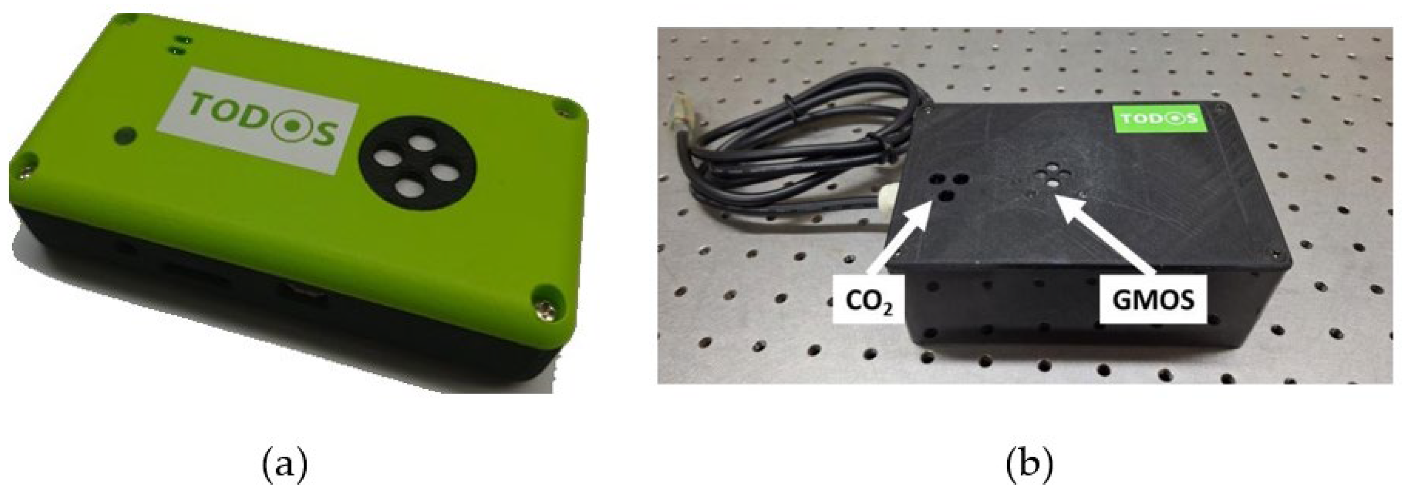
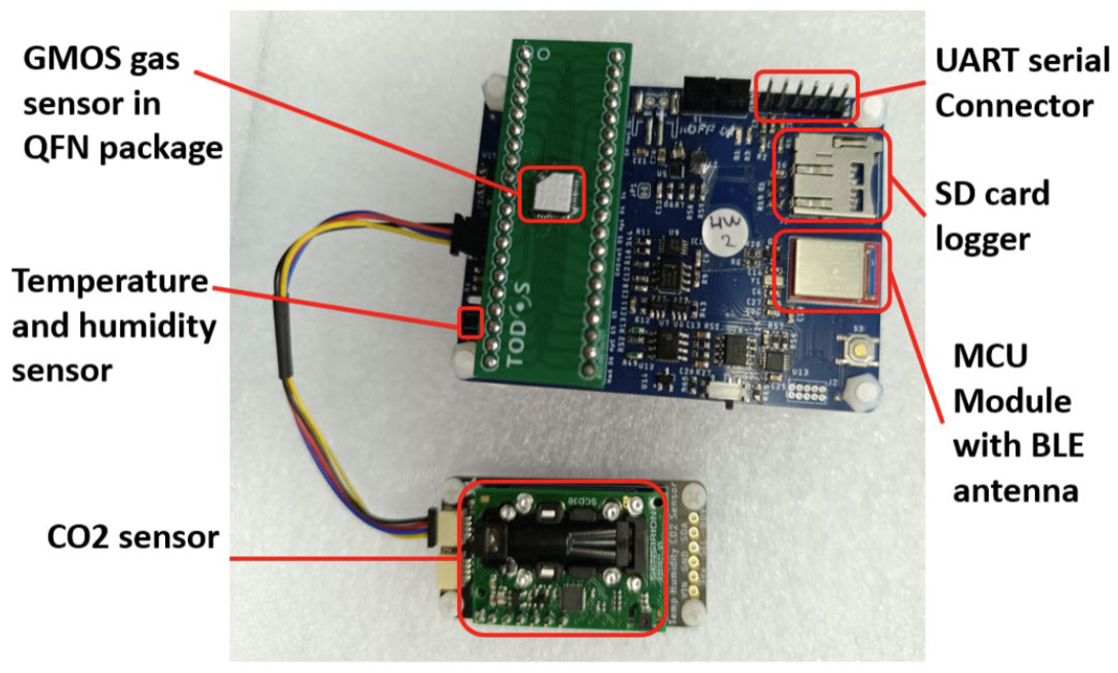
The organization of this paper is as follows: Section 2 details the hardware and data-collection setup of a multigas-sensing system based on the catalytic CMOS-SOI-MEMS sensor dubbed GMOS [15,16]. Section 3 defines the drift-removal task, presents the spectral–temporal TCNN, and notes TinyML deployment steps. Section 4 reports accuracy, memory, and latency for the float and quantized models. Finally, our conclusions are provided in Section 5. We now present the sensing platform and experimental setup used to evaluate our proposed approach.

2. Multi-Sensor System

2.1. Technology

A general view of the fully integrated GMOS sensor system is presented in Figure 1, with the fabrication flow shown in Figure 2. The GMOS dies are fabricated through wafer-level CMOS processing at a commercial foundry (XFAB, Erfurt, Germany), followed by the deposition of a catalytic nanoparticle layer at TODOS Technologies Ltd. (Airport City, Israel). The dies are then bonded, packaged in QFN-40 housings, and integrated onto a printed circuit board (PCB) for deployment. The analog front-end on the PCB digitizes the differential voltage signal using an ADC with a full-scale input range of 0–5 [V], establishing the effective dynamic range for all measurements. Still, the underlying sensing die is not a commercial part, but rather a research-stage prototype currently under development [16].

The core innovation of the GMOS sensor lies in its ability to selectively detect multiple gases based on physical rather than purely chemical mechanisms. Selectivity is achieved by measuring the exothermic heat released during gas combustion at near-ignition temperatures, rather than relying on gas-specific chemical reactions. This heat induces a temperature change that is sensed by a suspended transistor, thermally connected to a micro-heater and a catalytic surface. Each target gas exhibits a unique thermal response profile depending on the specific catalyst and operating temperature [17].

Each GMOS pixel incorporates a tungsten heating resistor to raise the catalyst temperature to ignition, often above 350 °C, depending on the target gas. This high-temperature operation desorbs surface moisture and supports consistent catalytic activity. Periodic thermal refresh cycles briefly elevate the temperature to 400 °C to remove contaminants and maintain stability. The catalytic layer used in this work is 0.5 μm platinum nanoparticle film, deposited by inkjet printing. Prior work [16] has shown that Pt nanoparticle catalysts offer nearly double the sensitivity of sputtered Pt films. More recently, Ashkar et al. [18] demonstrated that a bimetallic Pd-Pt bilayer catalyst deposited on GMOS pixels further enhances performance by reducing the ignition temperature and increasing sensitivity at low ethylene concentrations. The Pd-Pt catalyst also reduces the activation energy of the combustion reaction, enabling lower power operation and higher selectivity. These improvements make the GMOS system particularly effective for low-concentration ethylene sensing in humid, real-world environments.

2.2. Sensor Module and Communication

The assembled sensing system is shown in Figure 3. It includes the packaged GMOS sensors fitted with a hydrophobic gas-permeable filter (Cobetter X5H), along with CO₂, temperature and humidity sensors for environmental monitoring and compensation. The control electronics are built around a microcontroller unit (MCU) with BLE (Bluetooth Low Energy) support and additional components including the following:

• A UART (Universal Asynchronous Receiver–Transmitter) interface.
• An SD card logger for offline data storage.
• Power control and voltage regulation.

As shown in Figure 2b, the full GMOS sensor module supports two operational modes:

(1)

USB Mode: Data and power are transmitted over a single USB connection, allowing tethered operation and real-time logging to a host PC.

(2)

Wireless Mode (BLE): Sensor readings are wirelessly transmitted to a nearby device using BLE. In this mode, power is supplied via a battery or external power source, enabling autonomous in-field deployment.

The overall system is designed to support low-power, in situ, long-term deployments typical of precision agriculture applications, such as greenhouse monitoring, soil emission tracking, or early disease detection.

2.3. Data and Experimental Setup

To evaluate the GMOS sensor system under representative postharvest conditions, we conducted controlled experiments in a 6-L sealed acrylic chamber (Figure 4). The goal was to simulate the environment of degreening rooms, which are characterized by high humidity, elevated CO₂ levels, and exposure to low concentrations of ethylene gas. Several oranges were placed inside the chamber to emulate the CO₂ and humidity typically produced by fruit respiration, while ethylene gas was introduced externally from a certified bottle containing a 200 ppm ethylene-in-air mixture. The GMOS sensor module, which integrates the gas sensor, temperature, humidity, and CO₂ sensing, was positioned alongside the fruits.

Ethylene was introduced in stepwise concentrations ranging from 6 ppm down to 1 ppm, with 5-min intervals between steps. The concentration inside the chamber was calculated using $C_{ch}={\displaystyle \frac{C_0\cdot f\cdot t}{V_{ch}+f\cdot t}}$ where $C_{th}$ is the chamber concentration, $C_0$ is the source gas concentration, $f$ is the flow rate, $V_{ch}$ is the chamber volume, and $t$ is the injection time.

Figure 5 presents the results of this experiment. Figure 5a shows the GMOS sensor voltage response to ethylene at increasing concentrations. Figure 5b,c depict the corresponding relative humidity and ambient temperature inside the chamber. The system was able to detect as low as 1 ppm ethylene under challenging ambient conditions—specifically, relative humidity > 90% and CO₂ ≈ 6000 [ppm], which reflect the real-world operating conditions of postharvest sensing. The long-term CO₂ profile from the oranges is shown in Figure 6.

While short-term controlled tests like the above confirm the sensor’s ability to resolve low gas concentrations under humid, CO₂-rich conditions, long-term sensor deployments face an additional challenge: signal drift. Unlike the structured experiments in a sealed chamber, real-world agricultural monitoring often involves continuous, in situ sensing over days or weeks. During such prolonged measurements, the sensor baseline gradually shifts due to humidity absorption, temperature fluctuations, material fatigue, or contamination effects. This baseline drift can obscure true gas responses and degrade model performance unless it is actively compensated.

To illustrate the challenge of drift in practice, we conducted long-duration recordings under stable ambient air conditions, without introducing any target gas. Despite the absence of new chemical stimuli, the GMOS sensor signal exhibited a gradual and consistent baseline shift over time. Figure 7 highlights this phenomenon, showing how sensor drift can accumulate even in a static environment. This makes it increasingly difficult to distinguish true gas-induced responses from internal sensor dynamics, especially in long-term field deployments.

To better understand and address this issue, we collected a dedicated long-term drift dataset under controlled ambient conditions. This dataset captures the natural evolution of the sensor signal as it responds solely to environmental and internal factors over time, without gas injections or any known reference changes. It forms the foundation for training and evaluating our drift-compensation neural network, which aims to reconstruct the underlying drift-free signal in real time.

3. Drift Compensation Framework

3.1. Problem Formulation and Environmental Compensation

Gas sensor drift is the gradual, long-term deviation of a sensor’s baseline output due to aging, contamination, or environmental factors. Over time, this drift can mask or distort the true response to target gases, making sensor readings unreliable even under constant analyte conditions [3]. Formally, we model the raw sensor output as a sum of three components:

$$y\left[n\right]=x\left[n\right]+d\left[n\right]+\eta \left[n\right]$$

where $y\left[n\right]$ is the measured sensor signal at discrete time n, $x\left[n\right]$ is the true gas-induced response (the ideal signal in absence of drift), $d\left[n\right]$ is the drift (an additive low-frequency bias), and $\eta \left[n\right]$ represents measurement noise. In GMOS sensors, $\eta \left[n\right]$ is typically a combination of shot noise and low-frequency ${\displaystyle \frac{1}{f}}$ noise. While noise suppression partially addresses through soft-thresholding in the spectral domain (see Section 3.3), a deeper analysis of noise mechanisms is beyond our current scope. The drift component $d\left[n\right]$ typically varies much more slowly than the gas response $x\left[n\right]$. In other words, drift acts as a low-frequency contaminant in the sensor signal [8]. Our objective is to recover $x\left[n\right]$ from the corrupted measurements $y\left[n\right]$ in real time, treating drift removal as a signal denoising problem. Importantly, we do not attempt to predict or forecast future drift; instead, we focus on estimating and removing the drift present at time $n$, using only information up to that time (a causal filtering approach).

Before addressing drift removal, we first compensate for immediate environmental influences on the sensor. Factors like ambient humidity and temperature can alter the sensor baseline in a predictable way. We apply a lightweight polynomial correction to $y\left[n\right]$ based on the measured relative humidity ($RH$) and temperature ($T$), as the GMOS full system also measures these variables, partially removing environmental artifacts. Specifically, if $\overline{RH}$ and $\overline{T}$ denote reference ambient conditions (e.g., average humidity and temperature during calibration) and $\overline{y}$ is the nominal sensor baseline at those conditions, we define an environmentally compensated signal $y_{corr}\left[n\right]$ as

$$y_{corr}\left[n\right]=y\left[n\right]+k_{RH}\left(RH\left[n\right]-\overline{RH}\right)+K_T\left(T\left[n\right]-\overline{T}\right)-\overline{y}$$

Here $k_{RH}$ and $K_T$ are compensated coefficients (determined through calibration) that adjust the sensor reading for deviations in humidity and temperature, respectively. This linear model subtracts out the estimated baseline shift due to environmental fluctuations, yielding $y_{corr}\left[n\right]$ as an initial approximation of the true response. After this compensation, however, a residual drift component remains in $y_{corr}\left[n\right]$, arising from slow sensor aging, poisoning, or other unmodeled effects. It is this residual drift $d\left[n\right]$ (still present in $y_{corr}\left[n\right]$) that we aim to eliminate with our model.

We frame the drift removal as a signal separation and denoising problem: the sensor signal consists of a slowly varying baseline $d\left[n\right]$ and the fast-changing true signal $x\left[n\right]$ (along with noise). The key challenge is to distinguish and subtract the drift $d\left[n\right]$ without distorting $x\left[n\right]$. In classical signal-processing terms, one might apply a high-pass filter or baseline subtraction to remove low-frequency content. Here we take a data-driven approach, leveraging a spectral–temporal neural filtering model to learn this separation. We design a neural network that operates on the incoming sensor time series and produces an estimate $\widehat{x}\left[n\right]$ of the drift-free signal in real time.

3.2. Temporal Modeling with Causal TCNN

To estimate the drift $d\left[n\right]$ from the compensated signal in real time, we employ a Temporal Convolutional Neural Network (TCNN) with casual, dilated architecture. Causality means the model only sees past and present values; in practice, the model takes a window of past sensor readings as input, and outputs the predicted drift at the current time. In our implementation, the network processes a sliding window of 128 samples (covering a certain time span of sensor data) and produces a single scalar output $\widehat{d}\left[n\right]$, the drift estimate for the most recent data given. In real time, as new data comes in, the window shifts forward one step, and the network can evaluate again to update the drift estimate. This TCNN operates entirely causally: all convolution layers use one-sided (past-only) receptive fields, so at time $n$ the network never accesses samples at times > n. Causal convolutions ensure the model’s predictions can be used in live settings without peeking into the future [8].

The network architecture is a deep 1D convolutional network with dilated convolutions and residual connections, which is inspired by TCN structures for sequence modeling. Dilated convolutions allow the network to efficiently capture long-range temporal dependencies without using an excessively long filter kernel. Mathematically, a 1D dilated convolution with dilation factor $r$ and filter length $k$ computes an output $z\left[n\right]$ from input $u\left[n\right]$ as

$$z\left[n\right]=\sum _{k=0}^{K-1}w\left[k\right]\cdot u\left[n-r\cdot k\right]$$

where the filter taps skip r − 1 samples between each convolution operation. By increasing $r$ in deeper layers, the network’s receptive field grows with depth while keeping the number of weights manageable.

Our TCNN begins with a standard 1D convolutional layer (filter length 5) to extract local features from the 128-sample input window. After that, we stack multiple dilated Conv1D blocks: each block contains two causal dilated convolution layers (with ReLU activation), and a residual addition connecting the block’s input to its output. Stacking such layers gives the network a large effective memory. In our design, the number of convolutional filters per layer is kept relatively small (dozens of channels) to reduce complexity, yet the dilations let the model integrate information over the full 128-sample window for drift estimation. The final layer of the network is a simple 1 × 1 convolution (a pointwise linear layer with no activation), which maps the last block’s outputs to the single drift value $\widehat{d}\left[n\right]$. Essentially, the TCNN learns a function $f(\cdot )$ that predicts the current baseline offset, given recent sensor readings. By training on long-term sensor recordings, it adjusts its filters to recognize the slow patterns characteristic of drift.

The use of residual skip connections throughout the TCNN is helpful for performance. This architecture mitigates the vanishing gradient problem in deep networks and makes it easier for the model to represent an identity function if needed (i.e., output zero drift change) [19]. For our task, this is especially important because in the absence of significant drift, the network should ideally output $\widehat{d}\left[n\right]\approx \widehat{d}\left[n-1\right]$. The presence of residual connections was found to be beneficial, since the drift signal is very low-frequency [15], whereas any rapid changes in $y_{corr}\left[n\right]$ are likely due to gas reactions or noise. By using a deep, dilated CNN with these residual skips, the model can capture the long-term information, while being robust to short bursts or spikes in the signal.

3.3. Spectral Denoising via Hadamard Transform

Another feature of our framework is the integration of an orthogonal transform-domain filtering block within the neural network. The purpose of this block is to separate the slow drift component from higher-frequency fluctuations (gas response transients and noise) in a learned manner, by operating in the frequency domain. We implement this using a Hadamard Transform with learned soft thresholding. The Hadamard transform is an orthonormal, wavelet-like transform that breaks a signal into additive subcomponents of varying frequency content. In our model, the output from the convolutional layers is partitioned into fixed-length segments of length $N$ (chosen as a power of 2), and each segment is converted to the spectral domain by multiplying with an $N\times N$ Hadamard matrix $H$. Formally, if $u\in {\mathcal{R}}^N$ represents a segment of one feature map (i.e., a vector of $N$ consecutive time samples), the Hadamard transform produces

$${\mathcal{F}}_i=H\cdot u$$

The resulting vector $u$ contains the spectral components of the input segment. The first element of $u$ corresponds to the DC (low-frequency) component, where the subsequent elements correspond to progressively higher-frequency patterns in the segment. We then apply a soft-threshold nonlinearity to these transform coefficients: coefficients with small magnitude are attenuated or set to zero, while larger coefficients are preserved. This operation, often used in wavelet denoising, effectively filters out small oscillations presumed to be noise. The threshold value itself is not fixed; our network learns an appropriate threshold level (or, equivalently, a gating for each coefficient) during training, optimizing it to best separate drift vs. noise in the transform domain [20].

After thresholding, the modified coefficients $u$ are transformed back to the time domain by the inverse Hadamard transform (which for Hadamard is the same as the forward transform, up to a normalization factor). The output is a “cleaned” version of the original segment, with high-frequency noise substantially reduced. By inserting this module into the network, we encourage an explicit separation: the low-frequency content (which accumulates in the first few Hadamard components) is allowed to pass and contribute to the drift estimate, whereas the high-frequency content (spread across later components) is suppressed unless it is strong enough to exceed the learned threshold. This regularizes the drift estimate to remain smooth, a sensible assumption for long-term drift behavior. This transform operates with $O\left(NlogN\right)$ complexity and uses only additions/subtractions (no multiplications), which aligns with our low-cost, real-time requirements.

3.4. TinyML and the Model’s Quantization

Machine learning models have traditionally been designed for cloud computing or high-power edge devices, where memory and computational resources are abundant. However, many real-world sensing applications—especially in agriculture and environmental monitoring—require that intelligent processing happens locally, at the sensor node itself. These systems must often operate remotely, are battery-powered, and without reliable network connectivity.

TinyML is an emerging field that addresses this challenge, enabling the deployment of lightweight, efficient machine learning models directly onto resource-constrained microcontrollers (MCUs) and edge devices. TinyML models must achieve a delicate balance: they need to be powerful enough to perform non-trivial tasks like denoising, classification, or prediction, but small and efficient enough to fit within kilobytes of RAM and flash memory and execute inference in milliseconds using minimal energy [21].

For our application, where the GMOS sensor module must perform real-time drift compensation autonomously across diverse environmental conditions, adopting a TinyML approach is essential. Instead of relying on external servers for processing, we design our drift-correction model to run entirely on-board, ensuring robustness, lower latency, reduced communication bandwidth, and greater energy efficiency.

To achieve this, we first designed a compact Temporal Convolutional Neural Network (TCNN) that already minimizes computational cost through small kernels, shallow channels, and efficient transforms (Hadamard instead of Fourier or DCT). We then further optimized the model through 8-bit quantization, transforming it from a floating-point network into an integer-only model that can run efficiently on a standard microcontroller.

In the following subsections, we describe two quantization strategies explored in this work: Post-Training Quantization (PTQ) and Quantization-Aware Training (QAT).

For both quantization approaches, this process yields roughly a 4× reduction in model size (since float32 values are 4 bytes and int 8 values are 1 byte). This compression, combined with the model’s low computational complexity, makes real-time baseline correction directly on-device feasible, without reliance on external compute or communications. Such on-board processing not only reduces bandwidth and power usage, but also improves reliability in disconnected field scenarios.

3.4.1. Post-Training Quantization (PTQ)

In PTQ, the model is first trained in full precision (float32) and then quantized offline using TensorFlow Lite [19]. During this step, a small calibration dataset is used to determine appropriate scale and zero-point values for each tensor, effectively mapping the floating-point activation ranges into the signed int8 range (−128 to 127). All weights and activations are quantized, and we enforce symmetric quantization for inputs and outputs, to simplify inference. This method is straightforward and often sufficient [22].

3.4.2. Quantization-Aware Training (QAT)

To mitigate this potential loss, we also train a version of the model using Quantization-Aware Training (QAT). In QAT, “fake” quantization operations are inserted into the computational graph during training. This exposes the network to quantization noise throughout learning, allowing it to adapt its parameters to preserve performance post-quantization. QAT can achieve higher fidelity, because the model learns to compensate for the quantization effects, and in some cases the quantization acts as a form of regularization. However, QAT often needs more epochs and careful tuning to realize its benefits [22].

4. Drift Compensation Results and Discussion

This section quantitatively evaluates the proposed Hadamard-TCNN drift compensation framework under three deployment regimes: full-precision float32, 8-bit post-training quantization (PTQ), and 8-bit quantization-aware training (QAT). All models were evaluated on the held-out long-duration drift dataset (Section 2.3) of GMOS sensor recordings. In addition to accuracy, we report the memory footprint and single-sample inference latency for each model variant (

Table 1. Performance comparison of full-precision and quantized models for drift compensation. MAE is reported in both normalized units and physical scale (mV). Standard deviation (σ) is provided in mV. Latency refers to single-sample inference time on a desktop GPU (NVIDIA GeForce RTX 4070 Super).

Variant	MAE Normalized	MAE [mV]	Std [mV]	On-Disk Size [KB]	Latency [ms]
float32	0.00096	0.245	1.502	547.8	-
PTQ (int 8)	0.00335	0.856	4.323	154.2	46.659
QAT (int 8)	0.00437	1.116	8.286	182.2	46.936

). The float32 model serves as a baseline with highest precision and model size, while the PTQ and QAT models illustrate the impact of quantization on performance. Table 1 summarizes the mean absolute error (MAE), standard deviation, on-disk model size, and inference speed for the three model variants. Notably, quantization reduces the model size dramatically (from ~548 kB to ~154–182 kB) —a reduction of over 70%—which is critical for resource-constrained devices. The inference latency per sample is also very low for all models. On a desktop equipped with an NVIDIA GeForce RTX 4070 super GPU, the 8-bit quantized models execute in approximately 46–47 ms per inference (Table 1). These runtimes correspond to a processing rate well above the sensor’s sampling frequency (one sample per 2.4 s), confirming that our approach meets real-time requirements. While these latency measurements were obtained on a high-end PC, the TCNN’s compact architecture and integer-only quantization are designed specifically for microcontroller-class deployment. This suggests that the model can likely meet real-time constraints even on MCU hardware, given the sensor’s low sampling rate.

Despite the significant compression, the quantized models maintain a high level of accuracy. The float32 TCNN model achieves an MAE of 0.00096 (in normalized units), which corresponds to roughly ~0.245 mV error when converted to the sensor’s output scale (corresponding to <1 ppm of the target gas). The PTQ model has a slightly higher error (MAE ≈ 0.00335, in normalized scale), and the QAT model’s error is about 0.00437 (in normalized scale). In physical terms, these correspond to only around 1 mV of drift estimation error—an exceedingly small discrepancy, given that the raw sensor drift spans tens of millivolts over the recording. It is noteworthy that both quantization approaches preserve the prediction accuracy, reflecting the effectiveness of our TinyML optimization strategy. As discussed in Section 3.4, standard PTQ can introduce quantization noise that degrades model precision, whereas QAT trains the network to compensate for quantization effects. In our results, the PTQ model actually performed on par with (or even slightly better than) the QAT model in terms of MAE. Despite its purpose, the QAT model showed no significant accuracy advantage in this case.

This outcome may reflect the fact that both the drift dataset and network architecture are well suited to quantization, along with the fact that QAT typically requires more extensive fine-tuning to realize its full benefits. Importantly, neither quantized model exhibits any systematic bias in its predictions, and the increase in error relative to the float32 baseline is marginal. Quantitatively, we observe that the residual standard deviation increases only slightly, from approximately 1.502 mV for the float32 model to 4.323 mV (PTQ) and 8.286 mV (QAT) for the quantized models, due to the added quantization noise. Meanwhile, the mean error (bias) remains essentially zero for all models. However, the QAT model’s residuals do exhibit a noticeably larger spread compared to the PTQ model, indicating a higher variance in QAT’s prediction errors. This suggests that in our case, the quantization-aware training did not reduce the error variance—the QAT model even shows slightly more variability—whereas the PTQ model’s quantization noise remained relatively small.

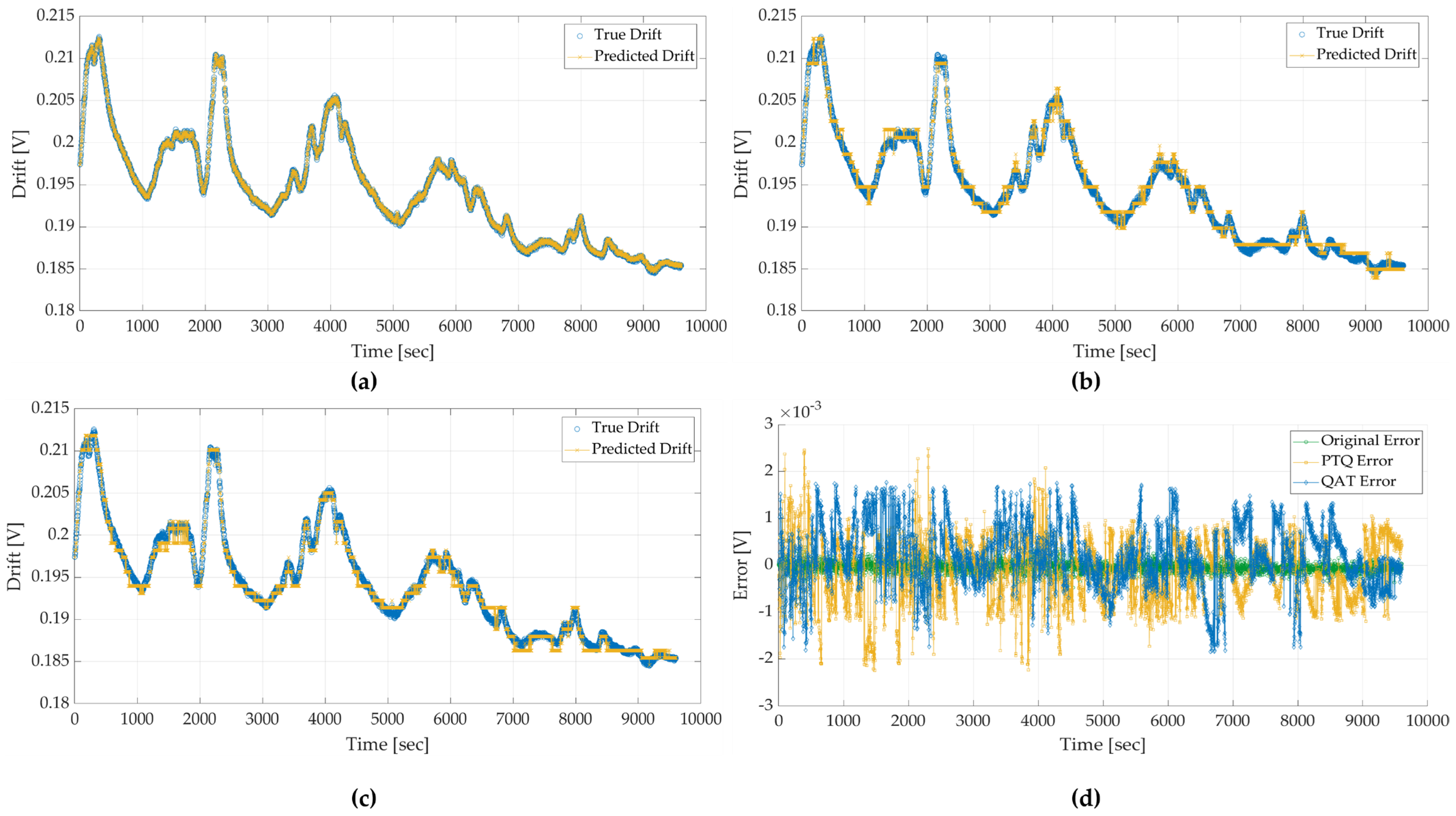
Figure 8 illustrates the model’s performance over time for each precision. In all cases, the TCNN’s predicted baseline (i.e., the drift-free signal) closely follows the ground-truth sensor output, which in this dataset reflects pure drift, since no external gas was introduced during recording. In Figure 8a, the full-precision float32 model’s prediction (blue line) is almost indistinguishable from the ground-truth drift (orange line), indicating virtually perfect compensation of the baseline wander. Figure 8b,c show the results for the quantized models (PTQ and QAT, respectively). The quantized models also capture the overall drift trend accurately, with only minor amplitude deviations. The fact that the orange and blue curves remain nearly overlapped in panels (b) and (c) demonstrates that quantization has not introduced any appreciable bias or lag in the drift prediction. In practical terms, all three models successfully reconstruct the slow baseline shifts over time, effectively removing drift to reveal a stable baseline. Panel 8(d) shows the instantaneous prediction error (in millivolts) across all three models. Overall, all three models effectively reconstruct the slow drift dynamics over time, validating that on-device inference, using only 8-bit arithmetic, achieves the same level of drift compensation as the original full-precision model.

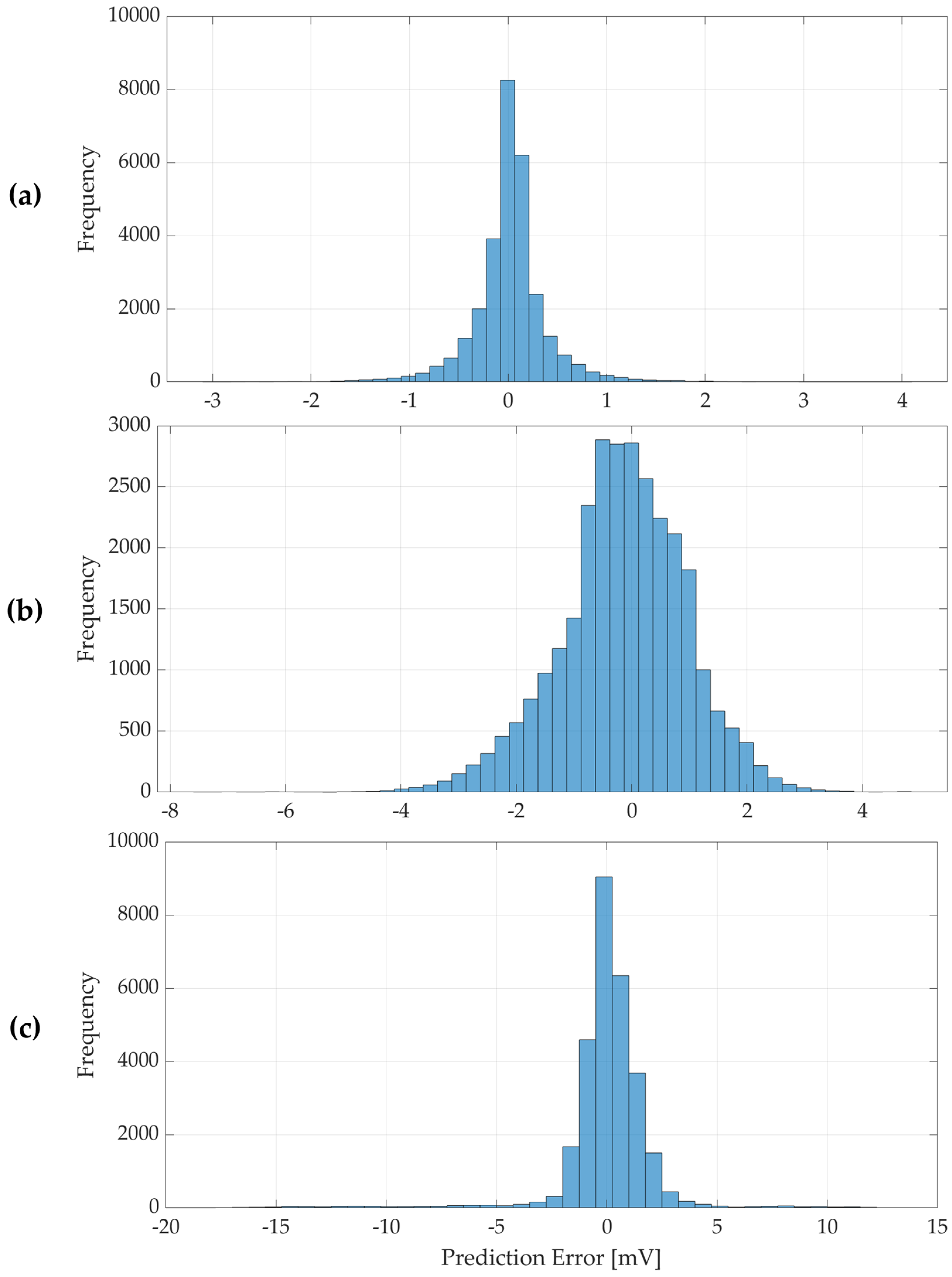
Figure 9 provides a complementary view by plotting the distribution of prediction errors (residuals = predicted drift minus true drift) for the float, PTQ, and QAT models. All three histograms are tightly centered at zero, underscoring the fact that the models do not consistently over- or under-estimate the drift (no bias). In Figure 9a (float32), the residuals cluster narrowly around 0, with a roughly Gaussian shape. The vast majority of errors are within ~0.25 mV, and the peak of the histogram is at 0 with a high frequency—indicating most predictions are nearly exact. For the PTQ model (Figure 9b), the error distribution broadens slightly: the spread of residuals increases. This reflects the quantization noise introduced by PTQ—effectively, a small random perturbation in the network’s outputs. The QAT model’s errors (Figure 9c) are likewise centered around zero (no bias), though its histogram exhibits slightly heavier tails (a few more outliers) compared to the PTQ model. Overall, the quantized models exhibit a minor increase in the variance of the error distribution compared to the float model, but no degradation in the mean accuracy.

In practical terms, these results demonstrate that our TinyML pipeline successfully translates a high-performance drift compensation model from full precision to an efficient integer deployment, with minimal loss of accuracy. The float32 model represents an upper-bound performance (with an absolute error well below 1 mV), and the quantized models perform nearly as well, with most errors remaining in the low single-digit millivolt range. Thus, the drift-corrected output from the quantized models closely matches the float32 model in practical terms. This finding is crucial for field deployment: it means we can reap the benefits of a 4× smaller model that can still achieve real-time execution on microcontroller-class hardware without sacrificing the sub-millivolt accuracy required for reliable gas sensing. The slight increase in error variance due to quantization is a reasonable trade-off for the substantial gains in memory efficiency and inference speed. Future implementations could further fine-tune QAT hyperparameters or apply calibration techniques to potentially close even this small gap, but our current results already validate the effectiveness of both PTQ and QAT for this application.

That said, the current drift training set was recorded under stable clean-air conditions, with temperature and relative humidity maintained within a narrow envelope ($\pm 2 °\mathrm{C} \mathrm{and} \pm 3\% \mathrm{R}\mathrm{H})$. While we apply a second-order polynomial pre-correction to remove deterministic T/RH dependencies, the model was not explicitly trained or tested under broader environmental variability. In practice, environmental variability may induce additional baseline effects not represented here. As such, generalization to dynamically changing climates—especially in real-world agricultural settings—remains an open challenge. Expanding the drift dataset to include long-duration recordings under variable temperature, humidity, and interfering gases will be essential to fully characterize model robustness and to support domain-invariant training.

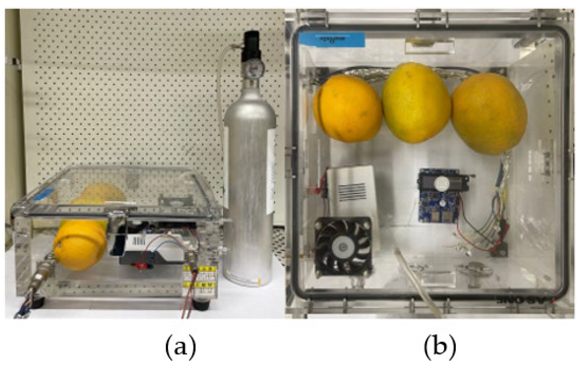
While this study focuses on long-term drift compensation, it also directly addresses two of the most persistent challenges in real-world gas sensing: selectivity and moisture resistance. These challenges are especially critical in fruit quality testing, where accurate ethylene quantification must occur in complex environments rich in interfering volatiles (e.g., terpenes from citrus) and under high humidity (>90% RH). The GMOS sensor employs a platinum nanoparticle catalyst operated at combustion temperatures, which inherently reduces humidity-induced variability by continuously desorbing surface-bound water and maintaining a clean catalytic interface. Periodic thermal refresh cycles further extend sensor stability by removing residual contaminants. Additionally, the sensor’s mechanism—measuring heat of reaction rather than surface resistance—provides a unique thermal signature for different gases, enhancing selectivity [12]. Recent findings by Ashkar et al. [18] further demonstrate that a Pd–Pt bimetallic catalyst layer on the GMOS architecture significantly enhances thermal stability, lowers ignition thresholds, and improves sensitivity to sub-ppm ethylene concentrations. However, even with these physical design advantages, baseline drift remains inevitable. Our contribution bridges this gap by integrating a real-time, on-device drift compensation model capable of learning and correcting these slow temporal shifts directly from the raw signal.

Compared to traditional drift mitigation techniques such as Papoulis–Gerchberg reconstruction [4], our approach offers significant advantages in flexibility and deployability. Classical methods often assume idealized drift profiles (e.g., smooth low-frequency trends) and require either future samples or regular recalibration with reference gases, limiting their real-time applicability. Machine learning models based on LSTMs or hybrid Transformer–LSTM structures [5,7] can better model nonlinear temporal dynamics, but typically require high memory and computational resources, making them impractical for on-device inference. In contrast, our drift compensation framework combines causal temporal convolutional layers with a lightweight Hadamard transform and residual gating to enable efficient, high-accuracy prediction using only past input. Furthermore, we demonstrate robust performance even after 8-bit quantization (both PTQ and QAT), with ~1 mV MAE and negligible bias, while enabling real-time execution on low-power microcontrollers.

5. Conclusions

This study demonstrates that baseline drift in low-cost gas sensors can be effectively mitigated entirely on-device by integrating a spectral–temporal neural filtering approach with a compact GMOS sensing platform. We introduced a causal TCNN architecture, enhanced with an embedded Hadamard transform, which suppresses high-frequency noise while preserving the slowly varying drift component critical to long-term sensor stability. Trained in full precision, the network achieved a mean absolute error below 1 mV on week-long drift recordings, confirming that the model can reconstruct the underlying gas response with near-laboratory accuracy.

To meet the stringent memory and power constraints of embedded deployments, the model was compressed using both post-training quantization (PTQ) and quantization-aware training (QAT) to an 8-bit integer format. This quantization reduced the model footprint from approximately 548 kB to under 185 kB, while enabling real-time inference with latencies of the order of tens of milliseconds (~46 ms per inference on an NVIDIA GeForce RTX 4070 PC). Importantly, predictive fidelity was essentially preserved—the quantized models’ accuracy remained within a fraction of a millivolt of the float model’s performance—demonstrating that TinyML techniques can deliver analytical-grade performance at the edge. These results demonstrate that real-time TinyML can offer reliable, maintenance-free drift correction, which is critical for deploying smart gas sensors in harsh agricultural settings.

Looking ahead, the quantized network is well-suited for embedding within a fully integrated, GMOS sensor system to achieve continuous, drift-corrected monitoring of sub-ppm ethylene levels on-device. Such an on-board deployment would eliminate the need for periodic manual recalibration or reliance on external cloud-based correction, paving the way for autonomous, real-time gas-sensing networks in food transportation containers, cold storage facilities, de-greening rooms, and directly in the field. Future work will focus on collecting long-duration drift traces under realistic and variable environmental conditions—including changing humidity, temperature and VOC mixtures—to extend the model’s robustness and support real-world deployment.