Abstract
Rhizoma Atractylodis macrocephalae (RAM) is a renowned food–medicine homologous herb in China, the quality and efficacy of which are inherently linked to its geographical origin. However, traditional origin identification methods for RAM are time-consuming, laborious, and destructive. This study introduces an innovative framework integrating hyperspectral imaging (HSI), broad learning system (BLS), and SHapley Additive exPlanations (SHAP) for RAM origin identification. RAM samples were collected from three origins, 100 samples from per origin, and imaged using a visible and short-wave near-infrared HSI system. BLS was used to build identification models with full and important wavelengths, and compared against seven traditional algorithms, including K-nearest neighbors (KNN), random forest (RF), support vector machine (SVM), back propagation neural network (BPNN), gradient boosting decision tree, (GBDT), extreme gradient boosting (XGBoost), and adaptive boosting (AdaBoost). Additionally, SHAP was used to enhance interpretability and identify important wavelengths highly correlated with RAM origin. Results showed that the full-wavelength BLS model achieved a test accuracy of 95.56%, which outperformed other models including KNN (77.78%), RF (85.56%), GBDT (88.89%), AdaBoost (90.00%), BPNN (91.11%), XGBoost (92.22%), and SVM (94.44%). SHAP identified important wavelengths similar to traditional methods (competitive adaptive reweighted sampling and successive projections algorithm), and the BLS model using SHAP-selected top 25 wavelengths achieved 94.44% accuracy with minimal performance loss. This study not only provides a rapid and accurate approach for RAM origin identification but also establishes a promising data-driven paradigm for non-destructive geographical origin traceability of other traditional Chinese medicines.
1. Introduction
Rhizoma Atractylodis macrocephalae (RAM), known as “Baizhu” in Chinese, is the dried rhizome of Atractylodes macrocephala Koidz., a plant belonging to the Asteraceae family [1]. RAM is one of famous traditional Chinese medicines (TCMs) and is often used as a food-medicine homologous product in China. As a kind of medicine and food homology material, RAM is highly prized for its diverse medicinal properties, like strengthening the spleen, benefiting vital energy, and eliminating dampness [2]. Moreover, studies show RAM also has other pharmacological activities such as anti-tumor, neuroprotection, and immunomodulation [3]. Currently, RAM is extensively cultivated in regions like Zhejiang, Anhui, and Sichuan in China [4,5]. It is widely acknowledged that the geographical origin affects the quality and efficacy of RAM [1,2]. However, due to the lack of corresponding industry standards for RAM, consumers cannot intuitively judge the geographical origin of RAM. Some illegal vendors sell low-quality RAM produced in some provinces as high-quality RAM herbs from Zhejiang to obtain high profits [2]. Therefore, it is urgent to develop a rapid and accurate method to identify the geographical origin of RAM.
Traditional methods for identifying the origin of TCMs mainly involve observing their physical characteristics, such as shape, color, and texture [6]. However, this method is highly susceptible to the interference of subjective factors of the identifiers. In addition, due to RAM from different origins are highly similar in appearance, it is often impossible to accurately identify them only by visual observation. At present, some physicochemical analysis methods have been reported for the origin identification of RAM, such as high-performance liquid chromatography (HPLC) [3], stable isotope [4], and plasma mass spectrometry [7]. For example, the mass spectrometry relative intensities of 46 mineral elements in combination with partial least squares discriminant analysis (PLS-DA), were used for the origin traceability of RAM [7]. Although these methods are accurate, they usually require complex experimental operation procedures, involving sample pretreatment, the use of various chemical reagents, and the assistance of large-scale instrument equipment [2,6]. Moreover, the operations are cumbersome and time-consuming, and the analysis costs are high, failing to meet the demands for rapid and efficient identification.
Hyperspectral imaging (HSI) is widely used in the field of agricultural products and food analysis, thanks to its unique strengths of non-destructiveness, high throughput, and high efficiency [8]. Unlike traditional single-point spectrometers that process samples one by one, HSI enables batch acquisition of optical information from samples. It also allows spectral extraction of target regions by selecting regions of interest (ROIs), which makes it suitable for the identification of RAM origins in this study. Generally, the analysis and processing of HSI data rely on machine learning algorithms. This is because these algorithms possess powerful capabilities in handling complex data patterns, extracting hidden features, and making accurate classifications [9]. In recent years, HSI combined with machine learning models such as the K-nearest neighbor (KNN), random forest (RF), and backpropagation neural network (BPNN) has been used for the geographical origin identification of various TCMs, such as ginseng [10], Pseudostellaria heterophylla [11], saffron [12], and wolfberry [13]. Although traditional machine learning models have achieved good results, there is still a need to explore new spectral identification model.
Broad Learning System (BLS) model is an emerging artificial intelligence algorithm proposed by Chen et al. [14]. It has attracted much attention due to its unique structural advantages and high-efficiency learning capabilities. By constructing feature nodes and enhancement nodes, it can rapidly process high-dimensional data and effectively avoid over-fitting, showing promising application prospects in many fields [15,16,17]. For example, BLS was integrated with near infrared spectroscopy for the identification of tobacco origin [18]. In another study, BLS was used for the classification of unsound wheat grains in terahertz images [19]. However, the application of BLS in identifying the origin of RAM and even in the entire field of TCMs is still relatively limited.
In addition, due to the complexity and high dimensionality of hyperspectral data, extracting important wavelengths to build simplified models is also a crucial step in spectral analysis. Traditional methods involve the use of variable selection techniques such as successive projections algorithm (SPA) [20], competitive adaptive reweighted sampling (CARS) [21], and VCPA-based hybrid strategy [22], to extract important feature wavelengths. For instance, CARS and SPA algorithms were applied to extract important wavelengths that are highly correlated with the origins of Radix pseudostellariae (a type of traditional Chinese medicinal herb) [11]. However, these methods prioritize predictive accuracy and generally lack the ability to explain the decision-making process of the model [23].
Currently, the model explainability has become one of the most studied topics in machine-learning-based applications, and explainable artificial intelligence (XAI) has become increasingly well-known [24]. SHapley Additive exPlanation (SHAP), which has received considerable attention, is a viable means to enhance model explainability because this explainable AI tool can quantify the relative importance of feature variables in the model [25]. As a model-agnostic approach based on game theory, SHAP has the capacity to generate feature attributions for every instance [26]. Such an ability is extremely valuable for achieving a more in-depth and thorough understanding of the model decision-making mechanism. Currently, several studies have used SHAP to explain their machine-learning models for spectroscopic data analysis. For example, the feasibility of SHAP in explaining the quality assessment model for sweet potato [24] as well as the classification model for wood species [27] has been proven. In this study, SHAP method was adopted to explain the RAM identification model and screen out the characteristic wavelengths that play an important role in the origin identification of RAM.
In summary, this study innovatively integrates the HSI, BLS, and SHAP techniques, and applies them to the geographical origin identification of RAM, aiming to develop a more accurate, efficient, and reliable identification method.
2. Materials and Methods
2.1. Sample Preparation
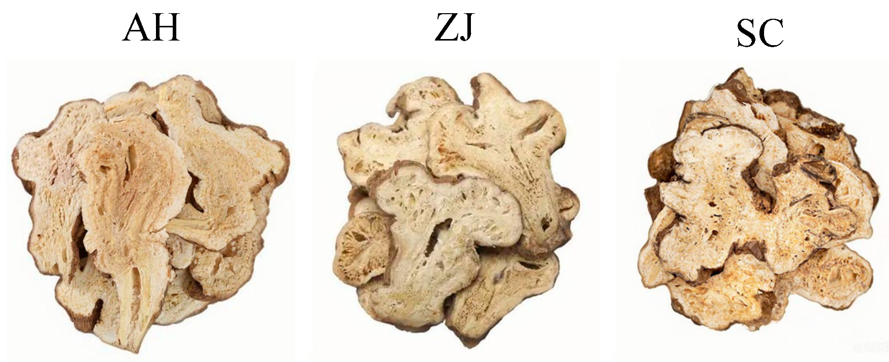
RAM samples collected from three geographical origins in China: Anhui province (AH), Zhejiang province (ZJ), and Sichuan province (SC). The 100 RAM samples per origin were purchased from local medicinal material markets of each origin. All were three-year-old specimens consistent with mainstream commercial specifications in the Chinese market, and had been processed into slices for commercial sale. Figure 1 presents the images of RAM from the three geographical origins. It is extremely difficult to distinguish RAM from different origins based on their appearance characteristics.

Figure 1.
RAM samples from different geographical origins.
2.2. Hyperspectral Imaging System
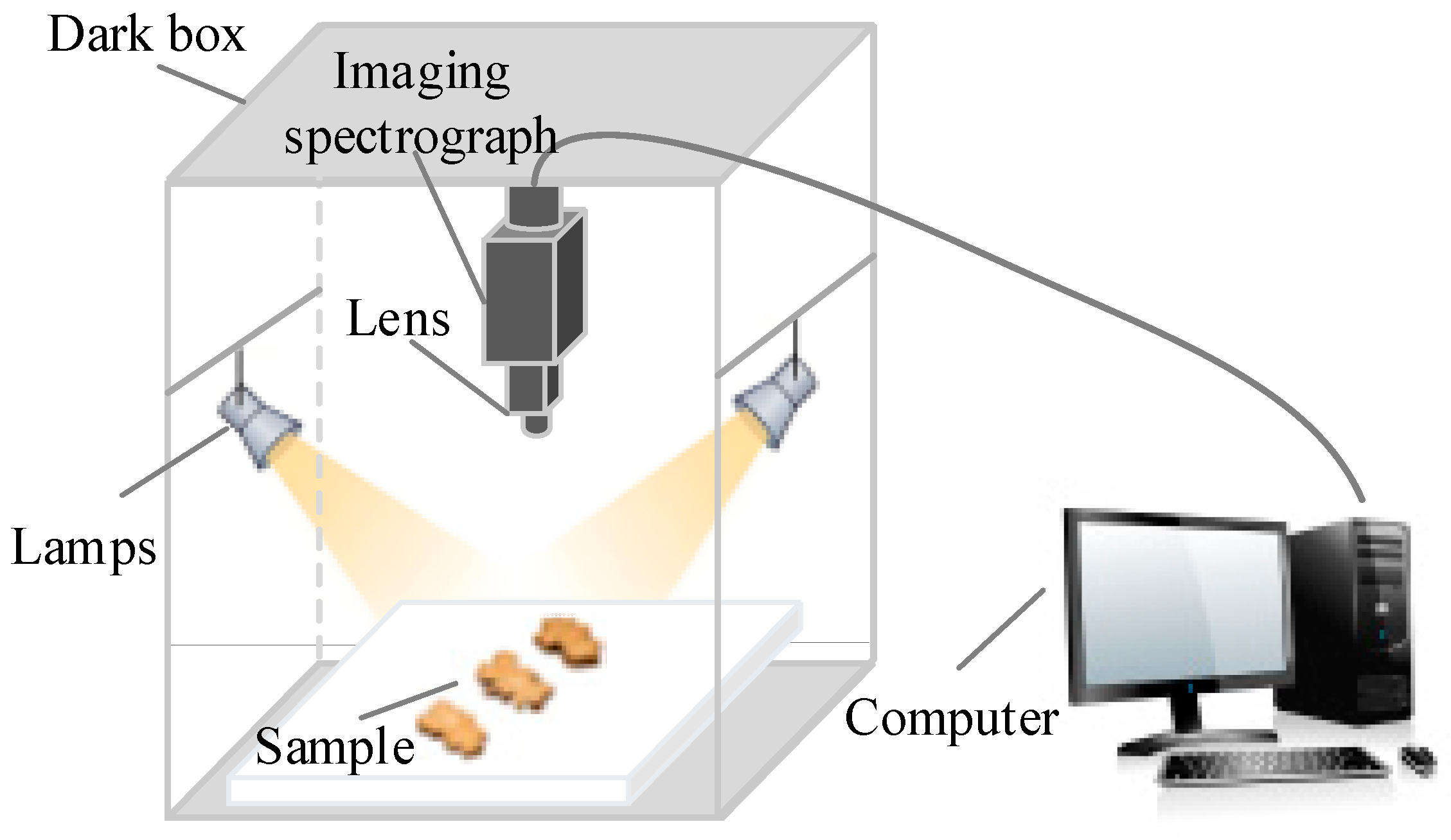
A hyperspectral imaging system was employed to collected hyperspectral images of RAM in reflection mode. As shown in Figure 2, the system works in the visible and short-wave near infrared range (397–1003 nm) and consists of an imaging module (Specim FX107, Specime imaging Ltd., Oulu, Finland), a set of 280 W halogen lamps (DECOSTAR 51S, Osram Corp., Munich, Germany), a mobile platform (HXY-OFX01, Red Star Yang Technology Corp., Wuhan, China), and a computer equipped with image acquisition software (Lumo Scanner, Specim, Spectral Imaging Ltd., Oulu, Finland). Before acquiring all sample images, the hyperspectral system was first preheated for 30 min. After the system stabilized, black-white board reference images were acquired once prior to measuring all samples, and these reference images were used to correct all subsequent sample images.

Figure 2.
Schematic diagram of hyperspectral imaging system for sample detection.
2.3. Spectral Data Extraction
All samples were imaged by the visible near-infrared hyperspectral imaging system. After RAM images were corrected, the entire surface of each RAM sample was identified as a region of interest (ROI); subsequently, the spectra of all pixels in the ROI were averaged to obtain a reference spectrum for the current sample. This approach was adopted with reference to the methods reported in References [6,11]. Therefore, a total of 300 spectra were obtained from RAM samples from three origins, and the spectral dataset was randomly divided into training set (210 samples) and test set (90 samples) in a 7:3 ratio. The 7:3 ratio was chosen because it balances sufficient sample size for the training set (to support feature learning) and the test set (to enable objective generalization evaluation). This is a widely used ratio in similar spectral classification studies [11].
2.4. Spectral Preprocessing Method
The collected spectral data is often affected by factors such as noise, scattered light, and baseline drift, which may affect the modeling effect [28]. An appropriate preprocessing selection can improve modeling accuracy, while an inappropriate selection can lead to a decrease in model prediction performance. However, the selection of an appropriate preprocessing method poses a challenge because the dimensionality and noise conditions are likely to fluctuate as the spectral data sets change [24]. In this study, six spectral preprocessing methods were used for the raw spectra, including Savitzky–Golay smoothing (SG), standard normal variation (SNV), multiple scatter correction (MSC), Savitzky–Golay first derivative (SG-D1), baseline correction (BS), and detrend (DT). SG smooths spectra via polynomial fitting, reducing noise while preserving features; SNV and MSC eliminate scattering interference from the sample surface [12]; SG-D1 combines SG smoothing and first derivative to reduce noise, eliminate baseline drift, and enhance component-related spectral peaks; BS eliminates background-induced baseline shifts to stabilize spectra baselines; and DT eliminates linear or slow nonlinear trends from instrument drift or sample placement. The optimal preprocessing method for raw spectra was determined by evaluating the classification accuracy of the built models.
2.5. Classification Model
2.5.1. Broad Learning System (BLS)
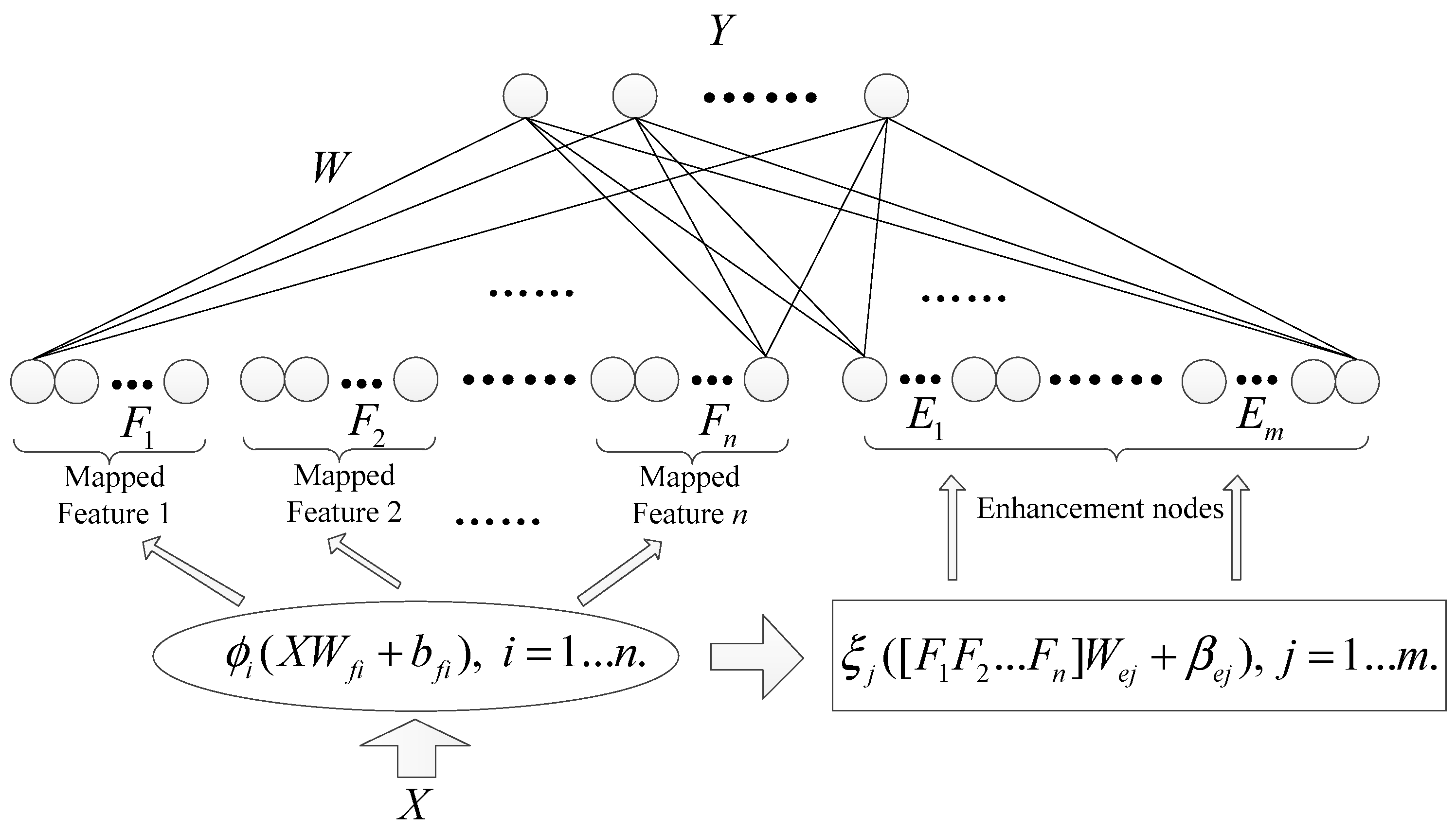
The BLS model [14] is a novel and efficient learning system, whose network structure consists of feature nodes and enhancement nodes, as shown in Figure 3. BLS model can quickly process large-scale high-dimensional spectral data, while effectively avoiding overfitting and improving generalization ability and stability by setting reasonable node parameters and connection methods within the model.
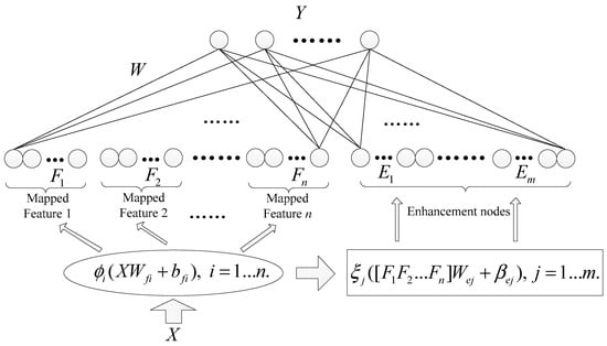
Figure 3.
Structure of BLS model.
To be more specific about Figure 3, the input X was spectral data, and then the X was mapped into n groups of feature nodes (), which were integrated to obtain the feature node set . Mathematically, it can be described as follows:
where represents mapping function, represents weight matrix, and represents bias matrix.
is further transformed in the enhancement layer to generate enhancement nodes (), which were integrated to obtain the enhancement node set . Mathematically, it can be described as follows:
where is a nonlinear activation function, represents weight matrix, and represents bias matrix.
Finally, the feature node and the enhancement node were connected together with the output Y, thus the output of BLS model can be described as follows:
where is the connection weight of the network.
Assuming , since Y (three geographical origin labels) was known, W can be represented as follows:
where is the inverse matrix of the input for the entire network, and please refer to the literature [14] for the specific calculation process of W.
2.5.2. Traditional Machine Learning Methods
In this study, the superiority of the BLS model was validated by comparing it with seven traditional machine learning models, including K-nearest neighbor (KNN), random forest (RF), support vector machine (SVM), backpropagation neural network (BPNN), gradient boosting decision tree (GBDT), extreme gradient boosting (XGBoost), and adaptive boosting (AdaBoost). Among them, RF, GBDT, AdaBoost, and XGBoost are classic tree-based ensemble learning algorithms, where RF employs a bagging strategy (combining multiple decision trees via random sampling) [29], while GBDT, XGBoost, and AdaBoost adopt boosting strategies (iteratively enhancing weak learners by focusing on misclassified samples). All integrate multiple weak learners to form a strong predictor [30]. Other models like KNN, SVM, and BPNN are standalone algorithms. KNN classifies via majority voting of nearest neighbors [31], SVM seeks optimal hyperplanes for classification, and BPNN updates weights through backpropagation in multi-layer architectures [32].
2.6. Shapley Additive Explanations (SHAP)
In explainable AI, SHAP is a tool used to explain the prediction results of machine learning models [24]. It is based on the Shapley value in game theory, which decomposes the model prediction results into various feature contribution values, namely SHAP values. Based on SHAP values, the positive and negative effects and degree of each feature on the prediction results can be clearly displayed, which helps to understand the decision-making mechanism of the model and improve its interpretability [26,27]. A detailed explanation of the calculation process for SHAP values can be found in the reference [26].
In this study, SHAP was used to explain the decision-making of KNN, RF, SVM, BPNN, GBDT, XGBoost, AdaBoost, and BLS models based on full-wavelength data. The mean absolute SHAP values were calculated to determine the significance of each spectral wavelength in the model outcome. The larger the SHAP value, the greater the impact of feature wavelength on the model classification results. Additionally, given that the number of full wavelengths was too large (224 features), only the top 30 important features were visualized. After that, secondary modeling was performed based on these important features to build the simplified models.
2.7. Traditional Wavelength Selection Methods
The competitive adaptive reweighted sampling (CARS) and successive projection algorithm (SPA) are two classic wavelength selection methods that effectively address the high-dimensionality of hyperspectral data by eliminating irrelevant, noisy, or collinear variables [33,34]. CARS is a variable selection method integrating Monte Carlo sampling with partial least squares regression model regression coefficients, which iteratively screens high-weight wavelengths and eliminates redundant variables [21]. SPA is a forward wavelength selection method dedicated to selecting wavelength combinations with minimal information redundancy to address collinearity issues [35].
2.8. Software
The extraction of RAM spectra was carried out using ENVI 5.2 software. The preprocessing, modeling and visualization of spectra were all carried out using the Anaconda 3 (Python 3.12) software.
3. Results
3.1. Raw Spectral Analysis
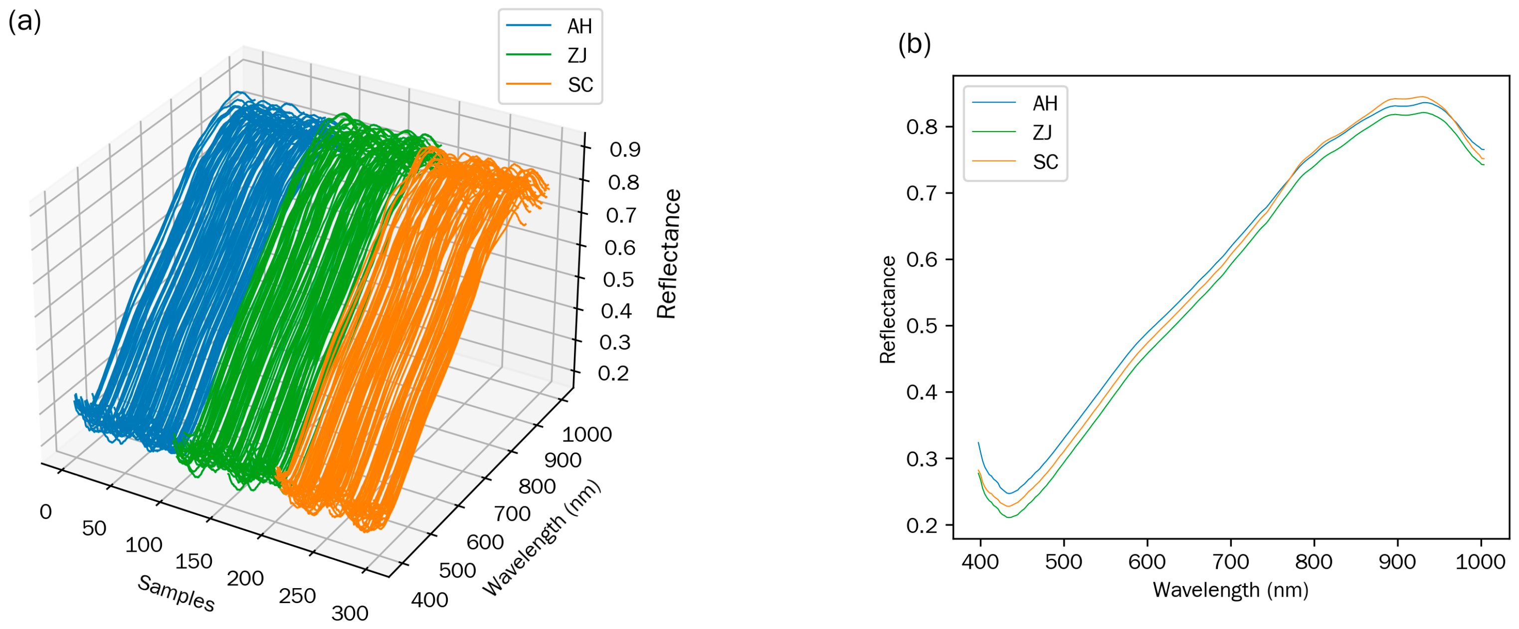
Figure 4 presents the raw spectra and average spectra of RAM from three origins. The comparison results showed that the variation trends of the spectral curves for the three origins were extremely similar. This similarity indicated that the material compositions of their main chemical components were alike [6]. Figure 4b depicts that the spectral reflectance slightly decreases within the 397–430 nm and then begins to rise from 430 nm. Notably, a distinct reflectance peak appears between 920 nm and 950 nm. This peak was probably caused by the second overtone of O-H stretching of water [36,37]. Furthermore, no significant peaks were identified in this study. This makes it challenging to identify RAM origin merely by visually examining the spectral characteristics. Therefore, it is imperative to conduct more in-depth analysis and processing of the spectra to explore the latent features concealed within the sample spectra.
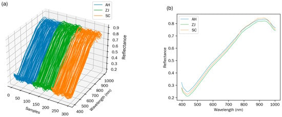
Figure 4.
Visualization of raw spectra for RAM samples of different origins: (a) Raw spectra; (b) Average spectra.
3.2. Principal Component Analysis for Raw Spectra
Principal component analysis (PCA), an unsupervised method commonly used in the exploratory analysis of spectra, was first applied to identify the raw spectra of RAM. Figure 5 shows the distribution of RAM samples from three different regions (AH, ZJ, SC) on principal component 1 (PC-1) and principal component 2 (PC-2). In Figure 5, the variance explained rates of PC-1 and PC-2 are 87% and 8%, respectively. The two components together reflect the main characteristic differences of the samples. The samples from different regions are represented by three types of markers with different shapes and colors. Although there is some overlap among them, they also show a certain degree of separation, indicating that the samples from each region have both similarities and differences in the feature space. Overall, PCA fails to accurately identify the RAM origin, since samples from different regions overlapping substantially. Therefore, the subsequent steps involve preprocessing the raw spectra and establishing a more accurate RAM origin spectral identification model.
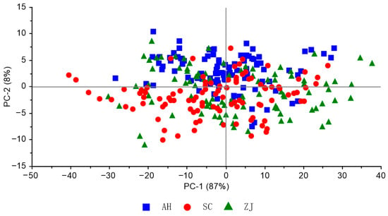
Figure 5.
PCA scores of RAM spectra from different origins.
3.3. Modeling Using Full Wavelengths
3.3.1. Spectral Preprocessing Analysis
The raw spectra and preprocessed spectra (SG, SNV, MSC, SG-D1, BS, and DT) were, respectively, imported into eight classifiers, including KNN, RF, SVM, BPNN, GBDT, XGBoost, AdaBoost, and BLS. A systematic comparison was conducted on the classification accuracy of different classifiers under various preprocessing methods. As shown in Table 1, the results indicated that spectral preprocessing methods (SG, SNV, MSC, SG-D1, BS, and DT) influence the performance of classifiers to varying degrees. This discrepancy arises because different preprocessing techniques target distinct spectral interference factors, leading to divergent action mechanisms that affect classifier performance [36]. Overall, SG-D1 outperformed other spectral preprocessing methods. This result is consistent with findings from similar study on the geographical origin identification of TCMs [11], primarily because SG-D1 integrates the advantages of Savitzky–Golay smoothing and first-order derivative, which suppresses spectral noise, eliminates baseline drift, enhances origin-related characteristic peaks, and thus improves subsequent models’ discriminative ability.

Table 1.
Classification accuracy of different models under various spectral preprocessing methods.
When SG-D1-preprocessed spectra were used as model inputs, the KNN, RF, SVM, BPNN, GBDT, XGBoost, AdaBoost, and BLS models achieved the highest accuracies of 77.78%, 85.56%, 94.44%, 91.11%, 88.89%, 92.22%, 90.00%, and 95.56%, respectively. Notably, BLS significantly outperformed traditional machine learning models, demonstrating the best classification performance across all preprocessing methods. Specifically, spectral data preprocessed by SG-D1, when fed into the BLS model, achieved 100% accuracy in the training set and 95.56% accuracy in the test set.
Figure 6 presents the RAM spectral reflectance map after SG-D1 processing. Compared with the gentle trend of the raw spectra (Figure 4), the SG-D1 processed spectra significantly highlighted the peak-valley features and local variations within the bands. This spectral feature enhancement enables the model to accurately capture key information in the data, thereby facilitating high-precision prediction. Consequently, SG-D1 preprocessed spectra were adopted for subsequent analysis.

Figure 6.
Visualization of pre-processed spectra for RAM samples: (a) SG-D1 pre-processed spectra; (b) Average spectra.
3.3.2. Model Comparison Analysis
As shown in Table 1, the BLS model achieves significantly higher accuracy than KNN, RF, SVM, BPNN, GBDT, XGBoost, and AdaBoost models, regardless of using raw or preprocessed spectra as inputs. This superiority originates from its unique network architecture, where feature nodes and enhancement nodes work synergistically, enabling efficient spectral feature extraction and reducing over-fitting risks in high-dimensional datasets [14]. By contrast, the KNN model shows lower test accuracy, likely because the algorithm exhibits high sensitivity to data distribution and vulnerability to noise and outliers [38]. Ensemble models (RF, GBDT, XGBoost, and AdaBoost) show robust training performance but unstable test accuracy, mainly caused by suboptimal parameter tuning (e.g., tree number/depth), leading to poor generalization [39]. While BPNN and SVM achieved over 90% accuracy in RAM origin identification and can model complex nonlinear relationships, both suffer from insufficient big-data fitting capabilities [40]. In summary, leveraging its architectural advantages in feature extraction and generalization, the BLS model offers a more robust solution for RAM origin identification.
3.3.3. Confusion Matrix Analysis
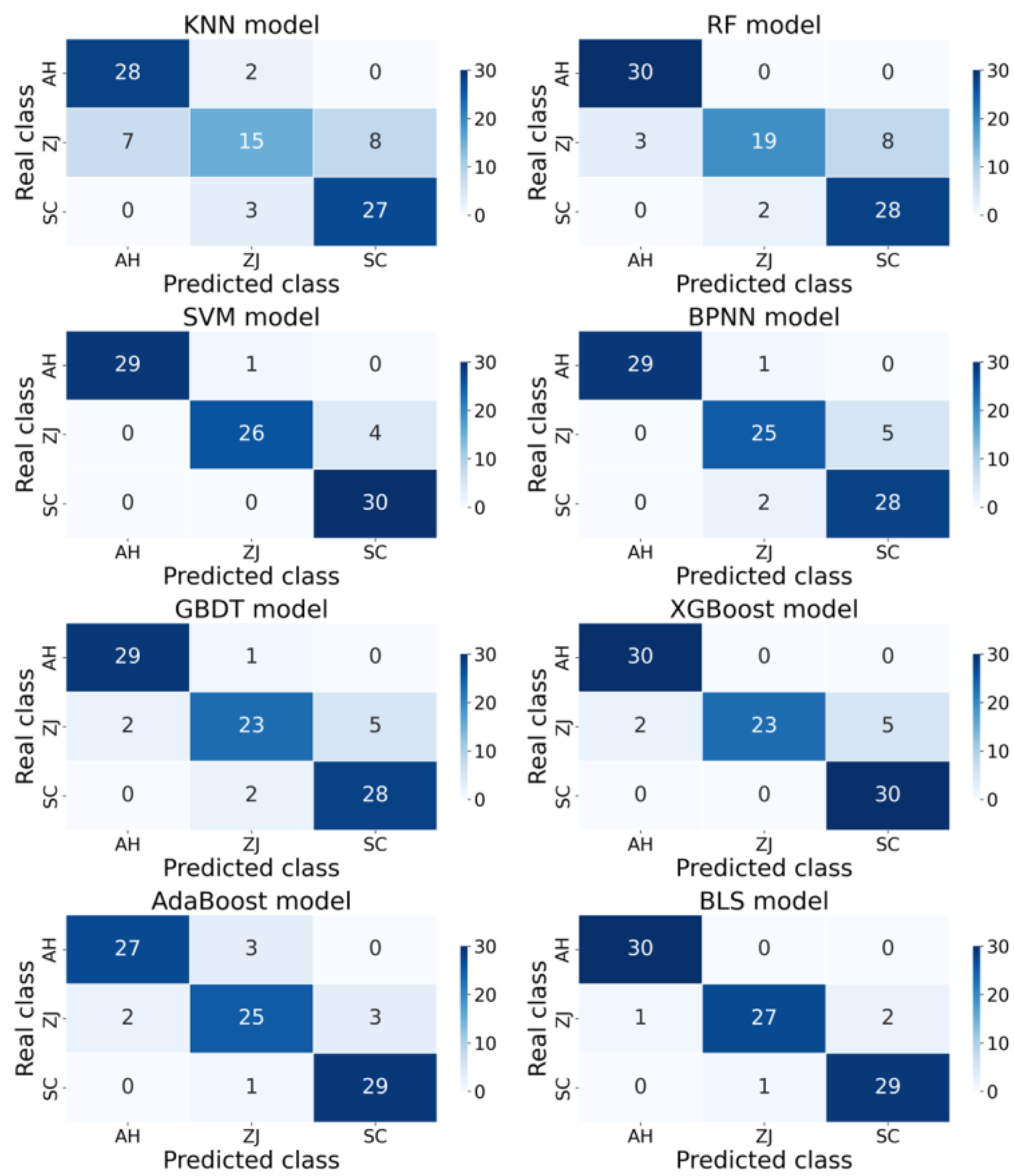
To intuitively and comprehensively analyze the classification performance of all models, confusion matrices for various models were plotted, as shown in Figure 7. A comparative analysis revealed that the numbers of misclassifications in the origin identification of RAM by the KNN, RF, SVM, BPNN, GBDT, XGBoost, AdaBoost, and BLS models were 20, 13, 5, 8, 10, 7, 9, and 4, respectively. Further observation of the confusion matrices of all models showed that RAM originating from ZJ was most prone to misidentification. Notably, compared with other algorithms, the BLS model performed exceptionally well in mitigating this issue, significantly reducing the misclassification rate of ZJ-origin RAM, which further highlighted its remarkable advantages in RAM origin identification tasks.
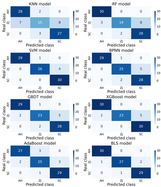
Figure 7.
Confusion matrices of multiple models for RAM origin identification based on the full wavelengths.
3.4. Model Explanation and Important Wavelengths Selection via SHAP
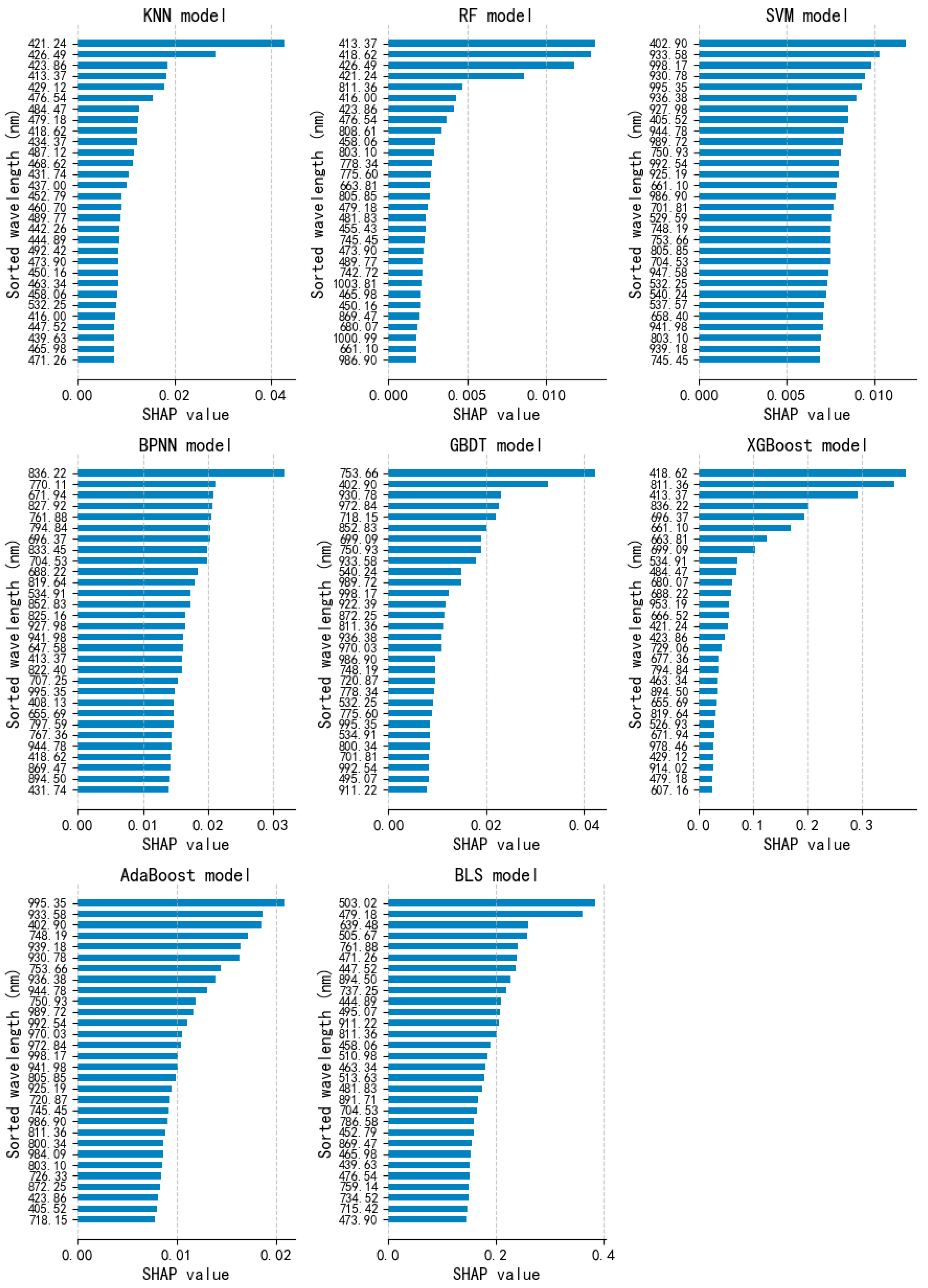
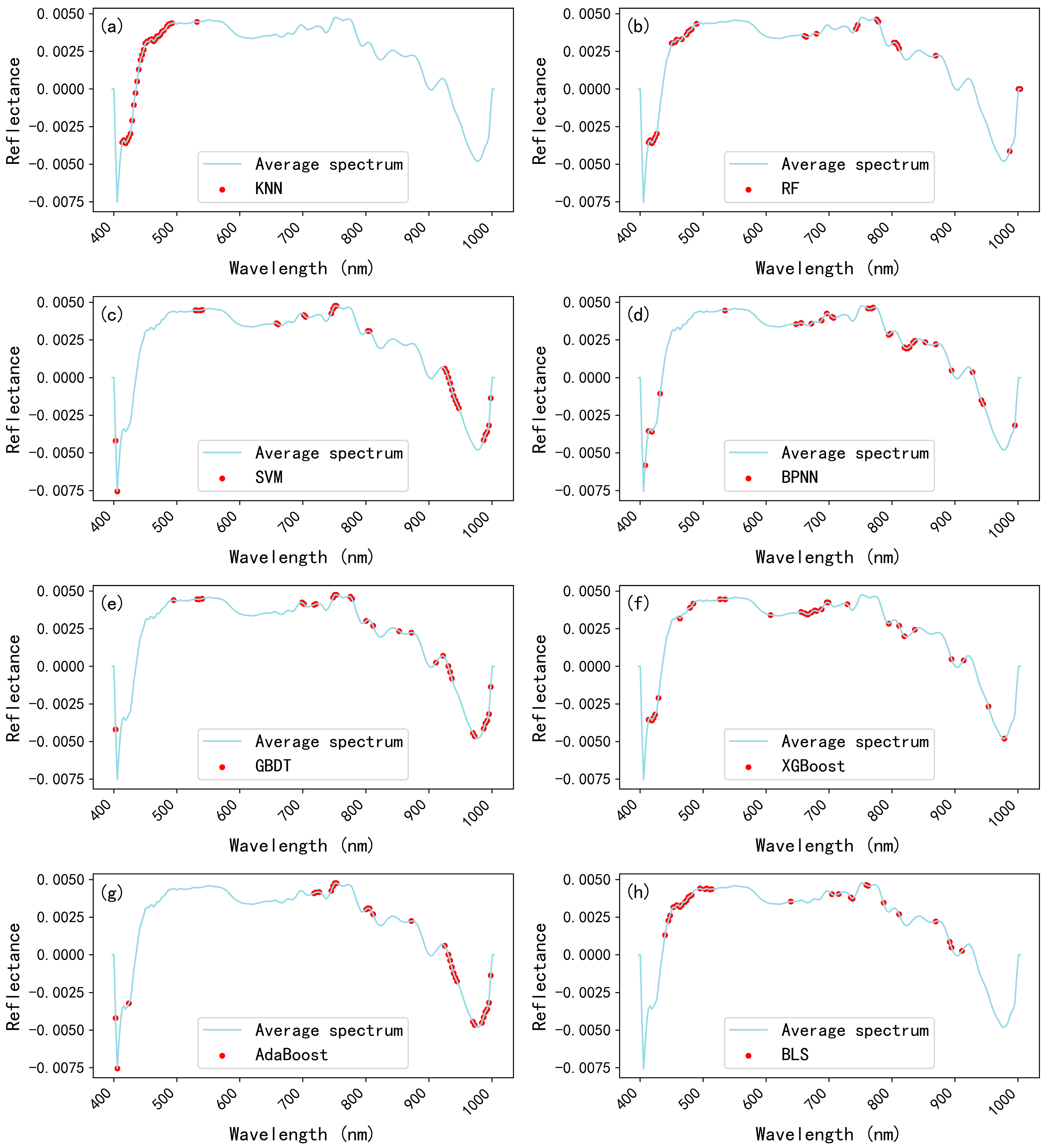
In this section, the SHAP method was applied to fulfill two critical objectives: interpreting model decisions and identifying important wavelengths associated with origins. Due to space limitations, Figure 8 only displays the SHAP values of the top 30 important wavelengths with significant impacts on model outcomes. Concurrently, Figure 9 illustrates the distribution of the top 30 important wavelengths identified by each model across the full wavelength spectrum. In Figure 8, comparative analysis revealed that the distributions of important wavelengths prioritized by different models varied substantially, thereby reflecting their distinct focuses in identifying RAM origins. In Figure 9, the KNN model tended to prioritize local spectral features, while other models (RF, BPNN, BLS, etc.) exhibited stronger capabilities in capturing broader-ranging feature information.
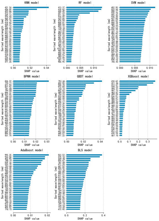
Figure 8.
Top 30 important wavelengths independently screened by each model (KNN, RF, SVM, BPNN, GBDT, XGBoost, AdaBoost, and BLS) based on SHAP explanation.
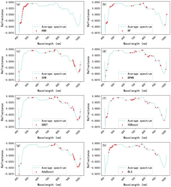
Figure 9.
Distribution of the top 30 important wavelengths identified via SHAP analysis for various models. In subplots (a–h), the blue line represents the average sample spectrum, while red dots denote wavelengths strongly affecting model output, reflecting their critical role in RAM origin identification.
Notably, despite the divergent working principles of the eight models, the analysis of important wavelength distributions (Figure 9) reveals that certain spectral bands are consistently identified as critical features across multiple models. This convergence suggests that these common bands play a fundamental role in RAM origin identification. In particular, the common bands are centered at approximately 413–513 nm, 639–811 nm, and 822–980 nm. It is well established that these bands correspond to overtone and combination vibrations of X–H groups (X=C, N, O) [41]. Previous studies have indicated that the pharmacologically active components associated with RAM predominantly include polysaccharides, atractylenolide I (A-I), atractylenolide II (A-II), atractylenolide III (A-III), and atractylone [1,6]. Importantly, polysaccharides and the atractylenolides (A-I, A-II, A-III) contain C–H and O–H functional groups [41], which likely contribute to the observed spectral features.
3.5. Important Wavelengths Selection Using CARS and SPA
After completing model interpretation and wavelength selection using SHAP, which clarified the contribution of each wavelength to model output, this research further employed CARS and SPA for wavelength selection. The subsequent sections conducted a comparative analysis of the wavelength ranges selected by these methods, with a primary focus on their consistency, dimensionality reduction efficiency, and classification accuracy. This analysis aimed to provide a multi-dimensional theoretical foundation for subsequent modeling.
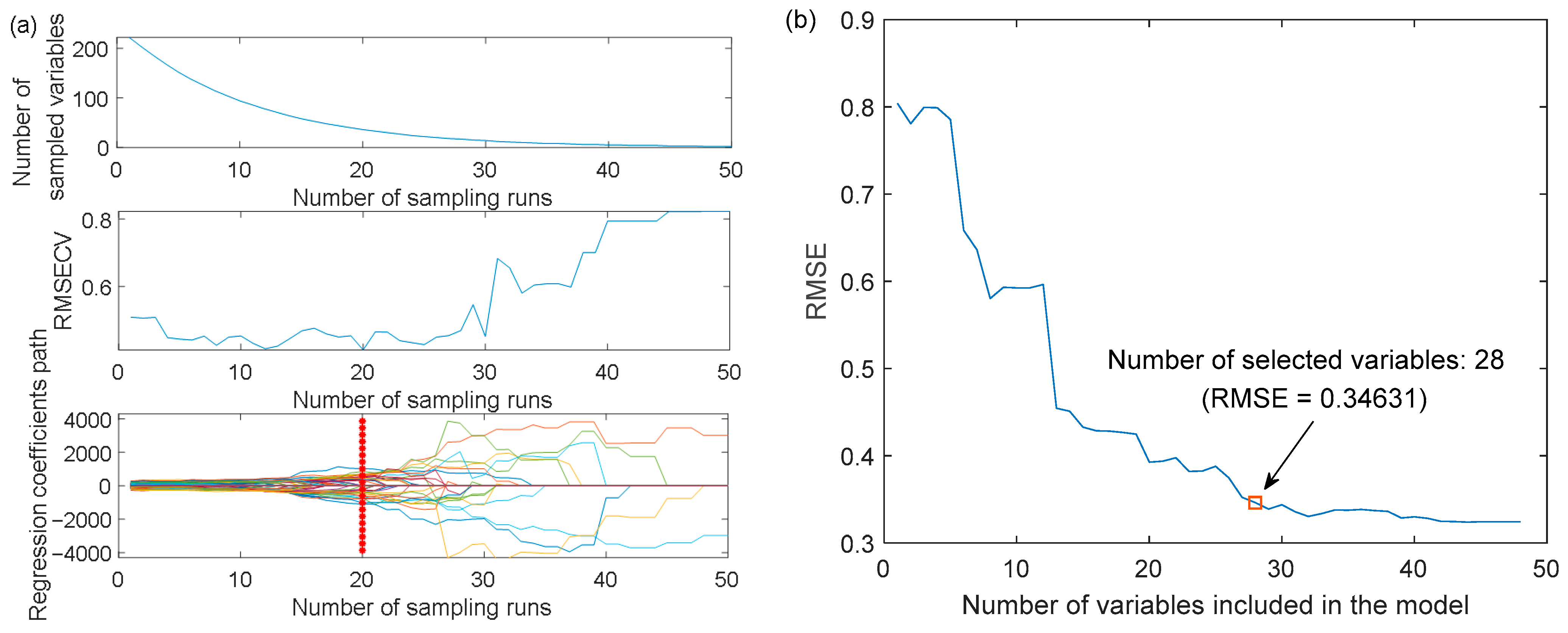
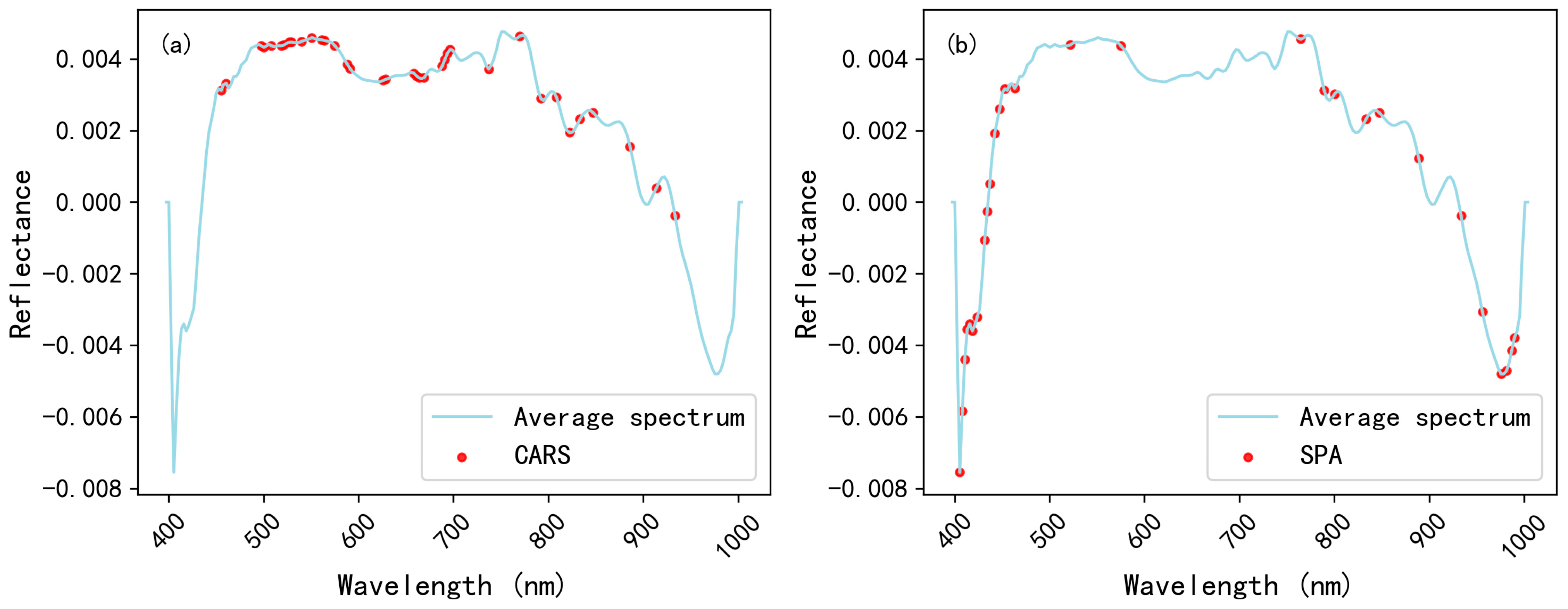
As shown in Figure 10a, the minimum root mean square error of cross-validation (RMSECV) was achieved at the 20th Monte Carlo sampling iteration (represented in red) in the CARS process. This demonstrated that the 36-variable subset selected at this stage effectively captured the spectral features critical for identifying RAM origins. In Figure 10b, the RMSE decreased with more variables added and then stabilized. The minimum RMSE (0.34631) occurred when 28 wavelengths were selected, meaning SPA identified these 28 wavelengths as the critical spectral information for RAM origin tracing. The specific distributions of important wavelengths extracted by the CARS and SPA algorithms across the full spectral range are described in Figure 11. By comparing Figure 9 and Figure 11, it is observed that the important wavelengths identified by the SHAP method show similarity to those extracted by CARS and SPA in distribution patterns.
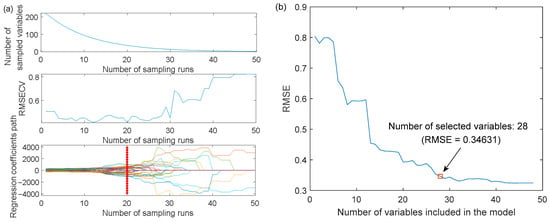
Figure 10.
Procedure for identifying important wavelengths via CARS and SPA methods: (a) CARS; (b) SPA.
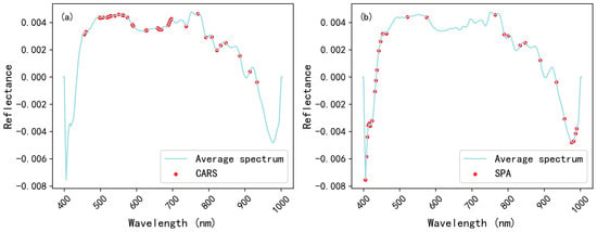
Figure 11.
Distribution of important wavelengths identified by CARS and SPA methods: (a) CARS; (b) SPA.
3.6. Modeling Using Important Wavelengths
Modeling with important wavelengths is critical to overcoming the high dimensionality of hyperspectral data. In this study, simplified classification models were developed using distinct subsets of important wavelengths: SHAP-selected wavelengths prioritized those deemed critical by the BLS model, while CARS and SPA employed algorithmic optimizations to identify subsets of 36 and 28 wavelengths, respectively. Table 2 presents their classification accuracy on the test set across eight machine learning algorithms (KNN, RF, SVM, BPNN, GBDT, XGBoost, AdaBoost, and BLS), highlighting the impact of wavelength selection methods on model performance.

Table 2.
Classification accuracy of different models based on SHAP, CARS, and SPA methods.
As shown in Table 2, the statistical results showed that the BLS model consistently outperformed traditional machine learning algorithms across all wavelength selection methods. Specifically, the SHAP-derived subset with 25 wavelengths achieved the highest accuracy of 94.44% in BLS. The SPA-selected subset with 28 wavelengths achieved 94.44% accuracy in BLS. Notably, these accuracies were slightly lower than the full-wavelength (224) BLS model (95.56%). Compared to SHAP and SPA, the CARS-extracted subset increased the wavelength count to 36; BLS achieved 95.56% accuracy with this subset, matching the accuracy of the full-wavelength BLS model. On the whole, although CARS demonstrated superior accuracy (95.56%) with 36 wavelengths, BLS paired with SHAP-selected wavelengths (25 wavelengths) offers a compelling trade-off: achieving 94.44% accuracy with fewer features and mechanistic interpretability. Therefore, by balancing model accuracy, explainability, and dimensionality reduction, BLS combined with SHAP emerges as the preferred strategy for RAM origin analysis, prioritizing robust model performance alongside scientific interpretability.
3.7. Model Deployment
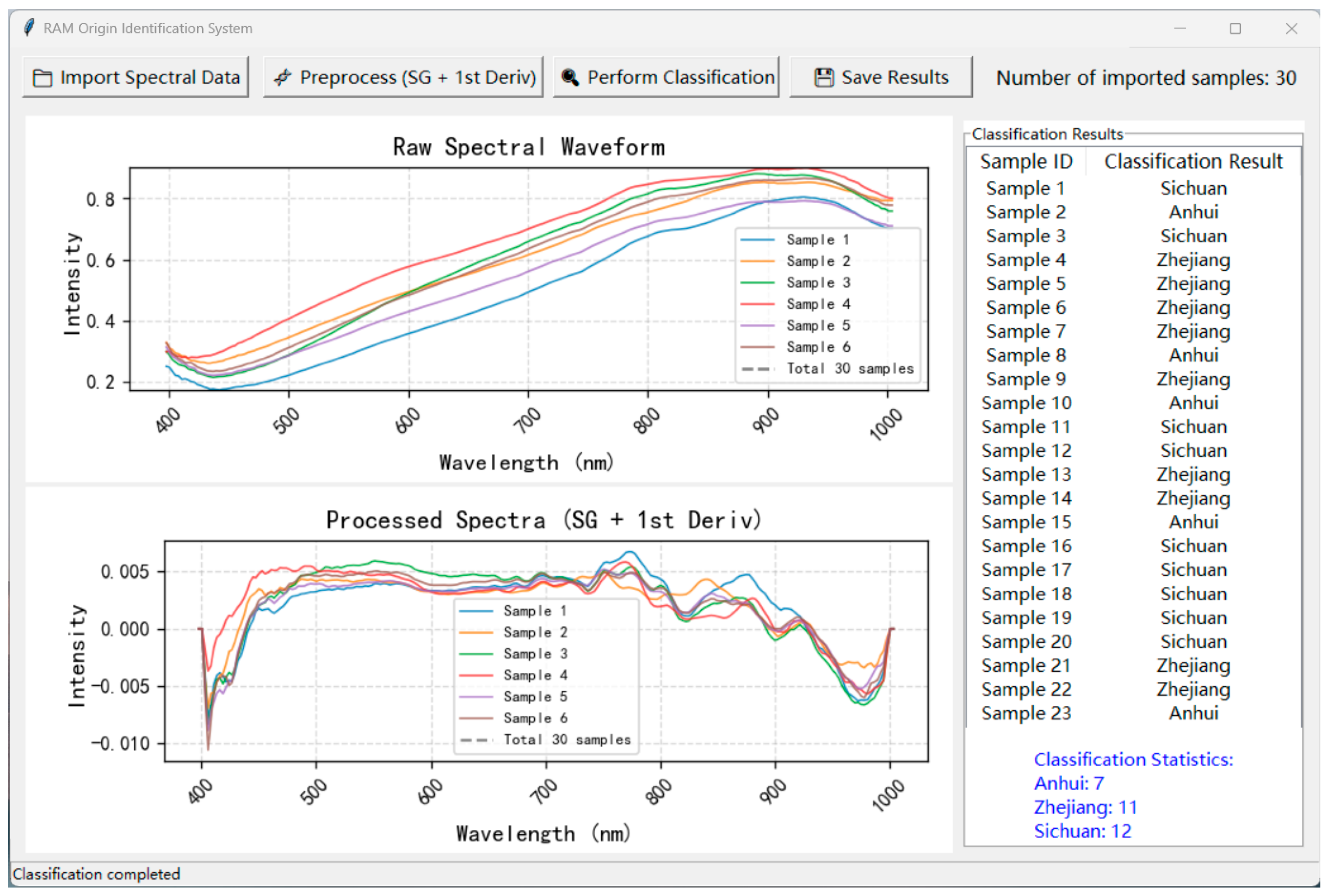
The RAM origin identification system deploys the trained BLS model through serialization, where the optimized model parameters and label encoder are saved as “bls_model.pkl” and “label_encoder.pkl” using the joblib library in Python. As shown in Figure 12, the system visually presents both raw and preprocessed spectra, outputs sample origin results through the classifier, provides statistical summaries, and enables the export of classification outcomes. This deployment approach ensures efficient model reuse, allowing the system to directly leverage pre-trained knowledge for RAM origin identification without retraining, which enhances the practical applicability and computational efficiency in real-world scenarios.
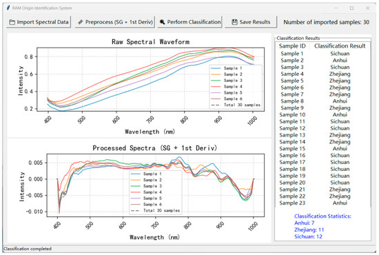
Figure 12.
RAM origin identification system.
4. Discussion
This study systematically demonstrated the feasibility of integrating HSI with the BLS model and SHAP technology for accurate origin identification of RAM origins, yielding highly satisfactory classification results. The full-wavelength BLS model achieved an accuracy of 95.56%, while the SHAP-selected top 25 important wavelengths enabled the BLS model to reach 94.44% accuracy. Although the accuracy achieved by modeling with selected important wavelengths was marginally lower than that of the full-wavelength model, the dimensionality reduction offered by wavelength screening remained crucial for enhancing model interpretability, computational efficiency, and providing a theoretical basis for the development of low-cost spectral systems for RAM origin identification [11,42,43]. More importantly, the identification of critical wavelengths facilitated a deeper mechanistic understanding of the intrinsic correlations between spectral signatures and RAM origins. It is worth noting that the important wavelength ranges selected by SHAP showed similarity to those selected by traditional wavelength selection methods (CARS and SPA), indicating that SHAP is capable of identifying wavelengths related to RAM origin while explaining model decisions. In general, SHAP is an “interpretation tool” that operates at the model level, with a core focus on “why a model makes such a prediction”; in contrast, CARS and SPA are “data dimensionality reduction tools” that are independent of the model itself, and their core concern is “which variables to select for modeling to achieve better results”. Currently, a growing number of studies tend to focus on how machine learning models make decisions, and SHAP has thus emerged as a favorable choice. For instance, SHAP has been used to explore wavelength relationships with rice milling quality [44] and identify important wavelengths linked to sweet potato quality [24]. However, this study applies SHAP to identify important wavelengths associated with the geographical origin identification of Chinese medicinal materials, which represents a meaningful and innovative exploration in this specific field.
As indicated in Table 1 and Table 2, the BLS model outperformed seven commonly used machine learning models, including KNN, RF, SVM, BPNN, GBDT, XGBoost, and AdaBoost. This finding aligns with previous research outcomes. For instance, studies on coal and tobacco origin identification using near-infrared spectroscopy both reported that the BLS model outperformed KNN, RF, SVM, and BPNN models in classification performance [18,45]. This might be attributed to its unique network structure and efficient feature-processing ability, which enabled the BLS model to quickly learn important features and conduct origin identification [14,17].
The current study highlights the potential of the BLS model in TCM origin identification. The preference for machine learning (ML) over deep learning (DL) is rooted in three practical constraints: limited dataset size (300 samples, insufficient for DL even with transfer learning due to the scarcity of large-scale TCM hyperspectral datasets), the low computational cost of ML, and the BLS model’s proven high accuracy. Although DL might marginally improve accuracy, this comes at the cost of substantially higher computational resources and model size. In future research, DL is considered as a justifiable alternative when faced with significantly expanded sample sizes or the need for multimodal information fusion (such as integrating spectral and image data) [46].
This study has limitations in the geographical coverage of RAM samples. In practical applications, when encountering samples from new origins, the model may face challenges of decreased accuracy in origin identification due to the lack of sufficient learning of comprehensive and regional representative features within a broader geographical scope. Therefore, expanding the geographical diversity of training samples to enhance the model’s generalization ability remains an important direction for future optimization. Moreover, it should be noted that the application of HSI in this study focuses on acquiring spectral information of target regions: spectral averaging is performed on each sample’s ROI pixels. In essence, this study does not fully utilize HSI’s ability to analyze spatial heterogeneity; instead, HSI is used as an “array spectrometer”. The core goal is to leverage its key spectral advantages, such as rapid batch acquisition and non-destructiveness, to meet the sample origin differentiation needs of this study. Future research can further explore the value of HSI’s spatial information, such as through pixel-level modeling and spatial feature extraction, to analyze how samples’ internal spatial heterogeneity affects detection results and more comprehensively exert HSI’s technical potential. Meanwhile, this study’s focus on RAM does not intend to suggest it is more difficult to identify by origin than all other medicinal plants. Instead, RAM was selected because it embodies the shared challenges of subtle morphological differences across origins and overlapping active component signals, challenges that are widespread in herbal medicine (e.g., in many widely used materials like Angelicae Sinensis Radix and Glycyrrhizae Radix et Rhizoma) and allow our findings to provide generalizable insights for origin identification beyond just RAM.
5. Conclusions
This study successfully demonstrated the feasibility of integrating HSI with the BLS and SHAP for rapid and accurate geographic origin identification of RAM. After systematic spectral pre-processing, full-wavelength modeling using multiple classification algorithms revealed that the BLS model achieved the highest classification accuracy of 95.56%, outperforming traditional machine learning methods such as KNN, RF, SVM, BPNN, GBDT, XGBoost, and AdaBoost. Leveraging SHAP for feature interpretation and selection, the top 25 important wavelengths were identified, with the BLS model achieving 94.44% accuracy using this subset. Notably, when compared with the CARS method, which achieved 95.56% accuracy using its selected wavelength set, SHAP demonstrated comparable effectiveness in dimensionality reduction while offering transparent insights into model decision-making. Overall, the HSI-BLS-SHAP framework presents a rapid, accurate, and interpretable solution for TCMs origin identification.
Author Contributions
Conceptualization, Methodology, and Writing—original draft, P.L.; Data curation, Project administration, and Writing—review and editing, H.L.; Formal analysis, Validation, and Writing—review and editing, D.L.; Data curation, and Writing—review and editing, L.H.; Investigation, and Visualization, C.L. All authors have read and agreed to the published version of the manuscript.
Funding
This research was supported by the Scientific Research Project of Fuyang Normal University (2024FSKJ31ZD, 2023KYQD0037, 2020KYQD0032), Industrial Chain Research and Innovation Team of Fuyang Normal University (CYLTD202213), Key Project of Scientific Research in Higher Education Institutions of Anhui Province (2023AH050385), and Open Fund of Anhui Engineering Research Center for Intelligent Computing and Information Innovation (ICII202305).
Institutional Review Board Statement
Not applicable.
Informed Consent Statement
Not applicable.
Data Availability Statement
Data are available on request.
Conflicts of Interest
The authors declare no conflicts of interest.
References
- Yang, R.; Wang, Y.; Wang, J.; Guo, X.; Zhao, Y.; Zhu, K.; Zhu, X.; Zou, H.; Yan, Y. Geographical Origin Traceability of Atractylodis macrocephalae Rhizoma Based on Chemical Composition, Chromaticity, and Electronic Nose. Molecules 2024, 29, 4991. [Google Scholar] [CrossRef] [PubMed]
- Chang, Y.Y.; Wu, H.L.; Wang, T.; Chen, Y.; Yang, J.; Fu, H.Y.; Yang, X.L.; Li, X.F.; Zhang, G.; Yu, R.Q. Geographical Origin Traceability of Traditional Chinese Medicine Atractylodes macrocephala Koidz. by Using Multi-Way Fluorescence Fingerprint and Chemometric Methods. Spectrochim. Acta Part A Mol. Biomol. Spectrosc. 2022, 269, 120737. [Google Scholar] [CrossRef] [PubMed]
- Tong, G.Y.; Wu, H.L.; Wang, T.; Chang, Y.Y.; Chen, Y.; Yang, J.; Fu, H.Y.; Yang, X.L.; Li, X.F.; Yu, R.Q. Analysis of Active Compounds and Geographical Origin Discrimination of Atractylodes macrocephala Koidz. by Using High Performance Liquid Chromatography-Diode Array Detection Fingerprints Combined with Chemometrics. J. Chromatogr. A 2022, 1674, 463121. [Google Scholar] [CrossRef] [PubMed]
- Hu, L.; Chen, X.; Yang, J.; Guo, L. Geographic Authentication of the Traditional Chinese Medicine Atractylodes macrocephala Koidz. (Baizhu) Using Stable Isotope and Multielement Analyses. Rapid Commun. Mass Spectrom. 2019, 33, 1703–1710. [Google Scholar] [CrossRef]
- Zhang, C.; Wang, H.; Lyu, C.; Wang, Y.; Sun, J.; Zhang, Y.; Xiang, Z.; Guo, X.; Wang, Y.; Qin, M.; et al. Authenticating the Geographic Origins of Atractylodes lancea Rhizome Chemotypes in China through Metabolite Marker Identification. Front. Plant Sci. 2023, 14, 1237800. [Google Scholar] [CrossRef]
- Ru, C.; Li, Z.; Tang, R. A Hyperspectral Imaging Approach for Classifying Geographical Origins of Rhizoma Atractylodis macrocephalae Using the Fusion of Spectrum-Image in VNIR and SWIR Ranges (VNIR-SWIR-FuSI). Sensors 2019, 19, 2045. [Google Scholar] [CrossRef]
- Wang, X.Z.; Chang, Y.Y.; Chen, Y.; Wu, H.L.; Wang, T.; Ding, Y.J.; Yu, R.Q. Geographical Origin Traceability of Medicine Food Homology Species Based on an Extract-and-Shoot Inductively Coupled Plasma Mass Spectrometry Method and Chemometrics. Microchem. J. 2022, 183, 107937. [Google Scholar] [CrossRef]
- Jiao, C.; Xu, Z.; Bian, Q.; Forsberg, E.; Tan, Q.; Peng, X.; He, S. Machine Learning Classification of Origins and Varieties of Tetrastigma Hemsleyanum Using a Dual-Mode Microscopic Hyperspectral Imager. Spectrochim. Acta Part A Mol. Biomol. Spectrosc. 2021, 261, 120054. [Google Scholar] [CrossRef]
- Ma, S.; Liu, J.; Li, W.; Liu, Y.; Hui, X.; Qu, P.; Jiang, Z.; Li, J.; Wang, J. Machine Learning in TCM with Natural Products and Molecules: Current Status and Future Perspectives. Chin. Med. 2023, 18, 43. [Google Scholar] [CrossRef]
- Cheng, R.; Bai, X.; Guo, J.; Huang, L.; Zhao, D.; Liu, Z.; Zhang, W. Hyperspectral Discrimination of Ginseng Variety and Age from Changbai Mountain Area. Spectrochim. Acta Part A Mol. Biomol. Spectrosc. 2024, 307, 123613. [Google Scholar] [CrossRef]
- Zhang, T.; Lu, L.; Song, Y.; Yang, M.; Li, J.; Yuan, J.; Lin, Y.; Shi, X.; Li, M.; Yuan, X.; et al. Non-Destructive Identification of Pseudostellaria heterophylla from Different Geographical Origins by Vis/NIR and SWIR Hyperspectral Imaging Techniques. Front. Plant Sci. 2024, 14, 1342970. [Google Scholar] [CrossRef]
- Kiani, S.; Yazdanpanah, H.; Feizy, J. Geographical Origin Differentiation and Quality Determination of Saffron Using a Portable Hyperspectral Imaging System. Infrared Phys. Technol. 2023, 131, 104634. [Google Scholar] [CrossRef]
- Xu, Y.; Wang, Y.; Cheng, P.; Zhang, C.; Huang, Y. A Lightweight Neural Network Approach for Identifying Geographical Origins and Predicting Nutrient Contents of Dried Wolfberries Based on Hyperspectral Data. J. Food Meas. Charact. 2024, 18, 7519–7532. [Google Scholar] [CrossRef]
- Chen, C.L.P.; Liu, Z. Broad Learning System: An Effective and Efficient Incremental Learning System Without the Need for Deep Architecture. IEEE Trans. Neural Netw. Learn. Syst. 2018, 29, 10–24. [Google Scholar] [CrossRef] [PubMed]
- Meng, J.; Huo, X.; Zhao, H.; Zhang, G.; Zhang, L.; Wang, X.; Lin, J.; Zhou, S. Multi-Modal Biological Feature Selection for Parkinson’s Disease Staging Based on Binary PSO with Broad Learning. Biomed. Signal Process. Control 2024, 94, 106234. [Google Scholar] [CrossRef]
- Men, J.; Zhao, C. An Adaptive Imbalance Modified Online Broad Learning System-Based Fault Diagnosis for Imbalanced Chemical Process Data Stream. Expert Syst. Appl. 2023, 234, 121159. [Google Scholar] [CrossRef]
- Huang, H.; Liu, Z.; Chen, C.L.P.; Zhang, Y. Hyperspectral Image Classification via Active Learning and Broad Learning System. Appl. Intell. 2023, 53, 15683–15694. [Google Scholar] [CrossRef]
- Wang, D.; Yang, S.X. Broad Learning System with Takagi–Sugeno Fuzzy Subsystem for Tobacco Origin Identification Based on near Infrared Spectroscopy. Appl. Soft Comput. 2023, 134, 109970. [Google Scholar] [CrossRef]
- Jiang, Y.; Wen, X.; Wang, F.; Ge, H.; Chen, H.; Jiang, M. Classification of Unsound Wheat Grains in Terahertz Images Based on Broad Learning System. IEEE Trans. Plasma Sci. 2024, 52, 4973–4982. [Google Scholar] [CrossRef]
- Hu, F.; Zhou, M.; Yan, P.; Li, D.; Lai, W.; Zhu, S.; Wang, Y. Selection of Characteristic Wavelengths Using SPA for Laser Induced Fluorescence Spectroscopy of Mine Water Inrush. Spectrochim. Acta Part A Mol. Biomol. Spectrosc. 2019, 219, 367–374. [Google Scholar] [CrossRef]
- Li, H.D.; Xu, Q.S.; Liang, Y.Z. LibPLS: An Integrated Library for Partial Least Squares Regression and Linear Discriminant Analysis. Chemom. Intell. Lab. Syst. 2018, 176, 34–43. [Google Scholar] [CrossRef]
- Yun, Y.H.; Bin, J.; Liu, D.L.; Xu, L.; Yan, T.L.; Cao, D.S.; Xu, Q.S. A Hybrid Variable Selection Strategy Based on Continuous Shrinkage of Variable Space in Multivariate Calibration. Anal. Chim. Acta 2019, 1058, 58–69. [Google Scholar] [CrossRef] [PubMed]
- Ahmed, M.T.; Kamruzzaman, M. Enhancing Corn Quality Prediction: Variable Selection and Explainable AI in Spectroscopic Analysis. Smart Agric. Technol. 2024, 8, 100458. [Google Scholar] [CrossRef]
- Ahmed, T.; Wijewardane, N.K.; Lu, Y.; Jones, D.S.; Kudenov, M.; Williams, C.; Villordon, A.; Kamruzzaman, M. Advancing Sweetpotato Quality Assessment with Hyperspectral Imaging and Explainable Artificial Intelligence. Comput. Electron. Agric. 2024, 220, 108855. [Google Scholar] [CrossRef]
- Marcilio, W.E.; Eler, D.M. From Explanations to Feature Selection: Assessing SHAP Values as Feature Selection Mechanism. In Proceedings of the 2020 33rd SIBGRAPI Conference on Graphics, Patterns and Images (SIBGRAPI), Porto de Galinhas, Brazil, 7–10 November 2020; pp. 340–347. [Google Scholar] [CrossRef]
- Lundberg, S.M.; Lee, S.I. A Unified Approach to Interpreting Model Predictions. In Proceedings of the 31st International Conference on Neural Information Processing Systems, Long Beach, CA, USA, 4–9 December 2017. [Google Scholar]
- Qi, Y.; Zhang, Y.; Tang, S.; Zeng, Z. Synergizing Wood Science and Interpretable Artificial Intelligence: Detection and Classification of Wood Species Through Hyperspectral Imaging. Forests 2025, 16, 186. [Google Scholar] [CrossRef]
- Jiang, Z.; Lv, A.; Zhong, L.; Yang, J.; Xu, X.; Li, Y.; Liu, Y.; Fan, Q.; Shao, Q.; Zhang, A. Rapid Prediction of Adulteration Content in Atractylodis Rhizoma Based on Data and Image Features Fusions from Near-Infrared Spectroscopy and Hyperspectral Imaging Techniques. Foods 2023, 12, 2904. [Google Scholar] [CrossRef]
- Zhang, Y.; Li, Y.; Zhou, C.; Zhou, J.; Nan, T.; Yang, J.; Huang, L. Rapid and Nondestructive Identification of Origin and Index Component Contents of Tiegun Yam Based on Hyperspectral Imaging and Chemometric Method. J. Food Qual. 2023, 2023, 6104038. [Google Scholar] [CrossRef]
- Demir, S.; Sahin, E.K. An Investigation of Feature Selection Methods for Soil Liquefaction Prediction Based on Tree-Based Ensemble Algorithms Using AdaBoost, Gradient Boosting, and XGBoost. Neural Comput. Appl. 2023, 35, 3173–3190. [Google Scholar] [CrossRef]
- Cheng, X.; Liao, M.; Liu, J. Geographical Origin Identification of Panax Notoginseng Using a Modified K-Nearest Neighbors Model with Near-Infrared Spectroscopy. IEEE Access 2025, 13, 13832–13846. [Google Scholar] [CrossRef]
- Dai, Y.; Yan, B.; Xiong, F.; Bai, R.; Wang, S.; Guo, L.; Yang, J. Tanshinone Content Prediction and Geographical Origin Classification of Salvia Miltiorrhiza by Combining Hyperspectral Imaging with Chemometrics. Foods 2024, 13, 3673. [Google Scholar] [CrossRef]
- Zhong, Q.; Zhang, H.; Tang, S.; Li, P.; Lin, C.; Zhang, L.; Zhong, N. Feasibility Study of Combining Hyperspectral Imaging with Deep Learning for Chestnut-Quality Detection. Foods 2023, 12, 2089. [Google Scholar] [CrossRef] [PubMed]
- He, H.; Chen, Y.; Li, G.; Wang, Y.; Ou, X.; Guo, J. Hyperspectral imaging combined with chemometrics for rapid detection of talcum powder adulterated in wheat flour. Food Control 2023, 144, 109378. [Google Scholar] [CrossRef]
- Liu, C.; Cao, Y.; Wu, E.; Yang, R.; Xu, H.; Qiao, Y. A Discriminative Model for Early Detection of Anthracnose in Strawberry Plants Based on Hyperspectral Imaging Technology. Remote Sens. 2023, 15, 4640. [Google Scholar] [CrossRef]
- Wang, Z.; Wan, X.; Luo, X.; Yang, M.; Wang, X.; Zhong, Z.; Tao, Q.; Wu, Z. Development of a Data Fusion Strategy Combining FT-NIR and Vis/NIR-HSI for Non-Destructive Prediction of Critical Quality Attributes in Traditional Chinese Medicine Particles. Vib. Spectrosc. 2025, 137, 103780. [Google Scholar] [CrossRef]
- Wan, X.; Luo, X.; Yang, M.; Li, Y.; Zhong, Z.; Tao, Q.; Wu, Z. An Accurate Prediction of the Physicochemical Properties of Traditional Chinese Medicine Granules Using a Multi-Source Data Model Fusion Strategy Based on Deep Ensemble Learning Algorithms. Microchem. J. 2025, 209, 112790. [Google Scholar] [CrossRef]
- Xing, W.; Bei, Y. Medical Health Big Data Classification Based on KNN Classification Algorithm. IEEE Access 2020, 8, 28808–28819. [Google Scholar] [CrossRef]
- Liao, M.; Wen, H.; Yang, L.; Wang, G.; Xiang, X.; Liang, X. Improving the Model Robustness of Flood Hazard Mapping Based on Hyperparameter Optimization of Random Forest. Expert Syst. Appl. 2024, 241, 122682. [Google Scholar] [CrossRef]
- Huang, J.; He, H.; Lv, R.; Zhang, G.; Zhou, Z.; Wang, X. Non-Destructive Detection and Classification of Textile Fibres Based on Hyperspectral Imaging and 1D-CNN. Anal. Chim. Acta 2022, 1224, 340238. [Google Scholar] [CrossRef]
- Chen, X.; Sun, X.; Hua, H.; Yi, Y.; Li, H.; Chen, C. Quality Evaluation of Decoction Pieces of Rhizoma Atractylodis macrocephalae by near Infrared Spectroscopy Coupled with Chemometrics. Spectrochim. Acta Part A Mol. Biomol. Spectrosc. 2019, 221, 117169. [Google Scholar] [CrossRef]
- Nirere, A.; Sun, J.; Yuhao, Z. A Rapid Non-Destructive Detection Method for Wolfberry Moisture Grade Using Hyperspectral Imaging Technology. J. Nondestruct. Eval. 2023, 42, 45. [Google Scholar] [CrossRef]
- Wang, S.; Bai, R.; Long, W.; Wan, X.; Zhao, Z.; Fu, H.; Yang, J. Rapid Qualitative and Quantitative Detection for Adulteration of Atractylodis Rhizoma Using Hyperspectral Imaging Combined with Chemometric Methods. Spectrochim. Acta Part A Mol. Biomol. Spectrosc. 2025, 327, 125426. [Google Scholar] [CrossRef]
- Tang, Z.; Ma, S.; Qi, H.; Zhang, X.; Zhang, C. Nondestructive Detection of Rice Milling Quality Using Hyperspectral Imaging with Machine and Deep Learning Regression. Foods 2025, 14, 1977. [Google Scholar] [CrossRef]
- Lei, M.; Rao, Z.; Li, M.; Yu, X.; Zou, L. Identification of Coal Geographical Origin Using Near Infrared Sensor Based on Broad Learning. Appl. Sci. 2019, 9, 1111. [Google Scholar] [CrossRef]
- Rane, N.; Paramesha, M.; Choudhary, S.; Rane, J. Machine Learning and Deep Learning for Big Data Analytics: A Review of Methods and Applications. Partn. Univers. Int. Innov. J. PUIIJ 2024, 2, 172–197. [Google Scholar] [CrossRef]
Disclaimer/Publisher’s Note: The statements, opinions and data contained in all publications are solely those of the individual author(s) and contributor(s) and not of MDPI and/or the editor(s). MDPI and/or the editor(s) disclaim responsibility for any injury to people or property resulting from any ideas, methods, instructions or products referred to in the content. |
© 2025 by the authors. Licensee MDPI, Basel, Switzerland. This article is an open access article distributed under the terms and conditions of the Creative Commons Attribution (CC BY) license (https://creativecommons.org/licenses/by/4.0/).

