Abstract
In recent years, the application of Deep Neural Networks to gas recognition has been developing. The classification performance of the Deep Neural Network depends on the efficient representation of the input data samples. Therefore, a variety of filtering methods are firstly adopted to smooth filter the gas sensing response data, which can remove redundant information and greatly improve the performance of the classifier. Additionally, the optimization experiment of the Savitzky–Golay filtering algorithm is carried out. After that, we used the Gramian Angular Summation Field (GASF) method to encode the gas sensing response data into two-dimensional sensing images. In addition, data augmentation technology is used to reduce the impact of small sample numbers on the classifier and improve the robustness and generalization ability of the model. Then, combined with fine-tuning of the GoogLeNet neural network, which owns the ability to automatically learn the characteristics of deep samples, the classification of four gases has finally been realized: methane, ethanol, ethylene, and carbon monoxide. Through setting a variety of different comparison experiments, it is known that the Savitzky–Golay smooth filtering pretreatment method effectively improves the recognition accuracy of the classifier, and the gas recognition network adopted is superior to the fine-tuned ResNet50, Alex-Net, and ResNet34 networks in both accuracy and sample processing times. Finally, the highest recognition accuracy of the classification results of our proposed route is 99.9%, which is better than other similar work.
1. Introduction
Gas recognition technology based on gas sensor array is widely used, playing an important role in many fields such as disease prediction [1,2,3], food safety [4,5,6], environmental monitoring [7,8], coal mine risk prediction [9], and so on. For example, Liu et al. [9] adopted the gas sensor array technology to identify and detect the concentration of carbon monoxide and methane released in the process of coal oxidation or spontaneous combustion. By capturing the slight change of gas release in the initial stage of coal oxidation and combining with an artificial neural network, the risk prediction ability in a coal mine has been greatly improved. Methane, ethanol, ethylene, and carbon monoxide are common flammable gases and are often mixed together in practical situations, such as in a chemical industrial park. Therefore, it is of practical significance to study the classification and identification technology of methane, ethanol, ethylene, and carbon monoxide based on gas sensor array.
Since the time series sensing data may contain redundant data or noise, the performance of the classifier largely depends on the input data representation. Efficient input data representation is the key to gas classification, which is helpful for training the classified gas model with efficient input data. For example, Pan et al. [10] proposed a new hybrid convolutional and recurrent neural network method to achieve fast gas recognition, extract valuable transient features contained at the beginning of the response curve, and finally achieve an identification accuracy of 84.06% within a response time as short as 0.5 s, and increase to 98.28% when the response time is 4 s. Pareek et al. [11] proposed a new 3DCNRDN (3D convolution neural-based regression dual network) to achieve gas quantitation and identification, with a classification accuracy of 94.37%. YongKyung et al. [12] proposed a new classification method for mixed gases, which is based on the representation of simulated images with several sensor specific channels and the Convolutional Neural Network (CNN) classifier. He et al. [13] proposed a new hybrid CNN-Bi-LSTM-AM network model based on Bayesian as an optimization algorithm to realize rapid gas identification. However, in the process of gas classification, they did not consider the possible redundancy or noise information in the time series sensing data and did not conduct smooth filtering and noise reduction pre-processing on the time series sensing data, which would lead to the decline of classification accuracy.
However, time series sensing data are characterized by relationships between different attributes, which makes it difficult to obtain complex information and temporal correlations from sensor responses. Scholars have proposed to encode the time series into different types of images for visual analysis, which enables computer vision technology to be used for time series classification. This idea provides a new perspective for us to solve the classification of time series sensing data. Donner et al. [14] proposed a new method to analyze the structural nature of the time series of complex systems. By constructing an adjacency matrix with predefined recursive functions, the time series can be interpreted as a complex network. Silva et al. [15] use recursive graphs as the representation domain of the time series classification and measure the similarity between the recursive graphs with the Campana-Keogh (CK-1) distance, which is a distance based on Kolmogorov complexity. A video compression algorithm is used to estimate the image similarity, which is a simple and parameterless time series classification method. Javed et al. [16] used different line graph techniques to analyze the performance of multiple time series and introduced a graphic awareness framework for multiple time series. These methods explore how to visualize the topology and intrinsic properties of the time series. However, their visualization process did not consider the integrity of the mapping between time series and visual cues, which would have resulted in a degradation of the classification performance. Wang et al. [17] proposed a new framework based on the Gramian Angular Summation/Difference Field (GASF/GADF) and Markov Transition Fields (MTFs) to encode time series into different types of images, which enables computer vision technology to be used for time series classification and interpolation. Liu et al. [18] used the Markov Transition Fields (MTFs) to visualize sensor responses into images. Combined with the Small-Scale Convolutional Neural Network (SSCNN), gas classification was further realized. Wang et al. [19] took the whole process of gas reaction as the feature map and used the mixed neural network to classify the gas, achieving a 95% classification accuracy. Inspired by this, we consider using the Gramian Angular Summation Field (GASF) method to encode the time series into two-dimensional sensing images. Because it contains time correlation and can maintain time dependence, it can be well applied in our experimental research.
A pattern recognition algorithm [20,21,22] is another key process of gas recognition. Ha et al. [23] apply the K-Nearest Neighbor (KNN) algorithm in combination with the Multi-Mode Principle Component Analysis (MPCA), which can be used for process monitoring and fault monitoring. Sun et al. [24] proposed a pattern recognition method based on the Local Mean Decomposition (LMD) envelope spectrum entropy and the Support Vector Machine (SVM) for classifying leakage aperture categories. However, all the above methods require feature extraction (typical features include response maximum value, response time, integral area under response curve, etc.) before pattern recognition, which undoubtedly increases the difficulty of achieving the target task. As artificial intelligence technology has made great progress in multiple fields, Deep Neural Networks (DNN) have achieved remarkable achievements in the field of artificial intelligence, such as computer vision [25], natural language processing [26], malware detection [27,28,29], etc. For example, Peng et al. [30] have designed a Deep Convolutional Neural Network (DCNN) to classify four gases. The recognition accuracy is 95.2%, and the training time is 154 s. It is far better than that of the Support Vector Machine (SVM) and the Multi-Layer Perception (MLP).
The main contributions of this study can be summarized as follows: We illustrate with examples how Deep Neural Networks can be applied to time series gas sensing data. We use a variety of filtering methods to pre-process the gas sensing response data for more efficient input data representations and to improve the performance of the classifier. After that, we adopted the GASF method to encode the gas sensing response data into two-dimensional images, and converted the classification and recognition based on the time series gas sensing data into the classification and recognition of two-dimensional sensing images, and finally realized the classification of methane, ethanol, ethylene, and carbon monoxide. In addition, the data enhancement technique is applied in the experimental study to further improve the performance of the classifier with relatively few data samples. Combined with fine-tuning the GoogLeNet classification network, gas data samples were trained and tested. We carried out a variety of comparative experiments under different experimental settings, including using the 10-fold cross validation method to verify the accuracy of the algorithm, whether the gas sample data are smoothly pre-processed, whether the data are data enhanced, dividing the dataset into different proportions, using different classification network models to identify the gas, comparing the experiments performed by other researchers on this dataset. The performances of the suggested algorithms in other UCI gas datasets are presented as well. The experimental results show that the Savitzky–Golay smooth filtering algorithm can greatly improve the performance of the neural network gas classification algorithm.
2. Materials and Methods
2.1. Materials
The data used in this experiment are an open-source gas dataset downloaded from UCI Machine Learning Repository public database [31]. The twin gas sensor arrays dataset is a time series gas sensor dataset of 8 sensor arrays. The dataset was collected by five identical sensor arrays, each containing four metal oxide gas sensors, namely TGS2611, TGS2612, TGS2610, and TGS26028. Each gas sensor operates at two heating voltage levels of 5.65 V and 5.00 V, resulting in a total of eight sensor combinations. The eight sensors are integrated in a specially designed circuit board, which is equipped with a temperature control and signal acquisition module to monitor the operation of the sensors. The experimental setup is shown in Figure 1 below.

Figure 1.
Experimental setup used for data acquisition.
During the signal acquisition process, the same experimental method was used to measure the gas of 5 sensor arrays, and the measurements were made with different sensor arrays every day. There are four types of gas tested, namely methane, ethanol, ethylene, and carbon monoxide. The duration of a single test experiment is 600 s, and the sampling frequency is 100 Hz. The types of sensors on a single sensor array and the working voltages of each sensor are shown in Table 1.

Table 1.
Sensor types and operating voltages.
The different concentration levels of the four measured gases are shown in Table 2.
Table 2.
Different concentration levels of measured gases (ppm).
The date of the detection of various gas substances of different concentrations by each sensor array is shown in Table 3.
Table 3.
The testing schedule for each batch of sensor arrays.
2.2. The Whole Experimental Process
The whole process of the experiment in this paper is as follows: First, in order to effectively extract the characteristics of the gas to be tested, the response data of the gas sensor were analyzed. The response data of the gas sensor within the range of important response and recovery time were retained, and the redundant and interference information was eliminated. Then, the time series data within the intercepted time range was visualized, and it was found that the response data of the gas sensor had certain data fluctuations and contained noise. Therefore, the smooth filtering method was considered to pre-process the data. In this paper, multiple smooth filtering methods were compared and analyzed, and the experimental results showed that Savitzky–Golay smooth filtering had the best classification effect. Therefore, Savitzky–Golay smooth filtering was selected for the basic experiment. Next, the GASF method was used to convert the pre-processed time series data into two-dimensional sensing images, and the data enhancement technology was used to reduce the impact of small samples on the classifier. In addition, the GoogLeNet classification network was fine-tuned to realize the recognition of four different gases, namely methane, ethanol, ethylene, and carbon monoxide. The flow chart of the whole experimental process is shown in Figure 2 below.

Figure 2.
The flow chart of the whole experimental process.
2.3. Data Pre-Processing
According to the literature [31], the specific collection experiment design of this gas sensor dataset is known. The experimental design of the four gases was the same, and the test time of a single experiment was 600 s. The process is as follows: First, constant flow of clean air is circulated through the gas sensor chamber for 50 s to form the initial stabilization phase of the response, which can be used as a baseline for measuring the sensor response. Secondly, the selected gas is passed into the sensor gas chamber and mixed with air according to the required concentration level to produce a gas mixture, which is circulated for 100 s. Finally, clean air is circulated to remove the gas mixture from the sensor chamber for the next 450 s.
The dataset used in this paper is 8 channels time series, , where , respectively, represents gas sensor array (TGS2611,TGS2612,..., andTGS2602) dynamic response data. Gas sensor array data are usually complex, high-dimensional time signals. To process such complex data, efficient input data representation is needed to complete the task of identifying gases. Since gas classification requires a large number of samples for model training, the performance of the classifier largely depends on the input data representation. Efficient input data representation is the key to gas classification and helps train the gas classification network model with input data. Otherwise, without proper input data representation, important information will inevitably be lost, which will degrade the performance of the classification model. In order to effectively extract the features of the gas to be identified, the data of the 8 channel time series are intercepted. In the experiment, the response data within 30–100 s are intercepted as the classification object. On the one hand, the response data within this time range includes both the gas response process and the gas recovery process, without losing the important response data in the gas reaction process. On the other hand, some redundant information is removed from the response data in this time range, which improves the efficiency of network model calculation. The original response data curve of CO gas is shown in Figure 3 below.

Figure 3.
The original response data curve of CO gas.
As can be seen from the above original response data curve of CO gas, the response of CO gas has certain data fluctuations and noise. In order to reduce the fluctuation of response data, a variety of smoothing filtering methods are used to pre-process the original gas response data. Based on the classification experiment results, Savitzky–Golay smoothing filtering algorithm has the best effect. Therefore, Savitzky–Golay smoothing filtering algorithm is mainly used in the following years. It is a function commonly used in curve smoothing processing and is a convolution algorithm based on smoothing time series data and the least squares principle. The core idea is to carry out order polynomial fitting to the data points in a certain length window, so as to get the fitting result. Savitzky–Golay smoothing filtering (SG smoothing filtering) is actually a weighted average algorithm for moving windows, but its weighting coefficient is not simply a constant window, but a least square fitting for a given higher-order polynomial within a sliding window.
The principle of Savitzky–Golay smoothing filtering is as follows: It is assumed that the width of the sliding time window is n = 2m + 1, and the data point is x = (−m, −m + 1, …, m − 1, and m). The sub-polynomial is used to fit the data points in the time window. The k − 1 degree polynomial is used to fit the data points in the window, y = a0 + a1x + a2x2 +...+ ak−1xk−1. Therefore, n linear equations with k elements are obtained. In order for the system to have a solution, n should be greater than or equal to k. Generally, n greater than k is selected, and the parameters are fitted by the least square method, A = {a0, a1, …, ak−2, ak−1}.
The biggest feature of Savitzky–Golay smooth filtering is that while filtering noise, it can ensure that the shape and width of the signal remain unchanged, which can better retain the information of characteristic peaks and improve the accuracy of input data. Therefore, based on the advantages of the Savitzky–Golay smooth denoising algorithm mentioned above, it can be well applied to the gas sensor dataset. As for the selection of experimental parameters, we compared the influences of different parameter selection on the gas classification results, as shown in Table 4. When window length increases from 29 to 89, the accuracy first increased, and then decreased. The time consumed kept on increasing when the window length increased. Window length of 59 provides better accuracy with little time as well. Based on the experimental results, this paper selects window length as 59 and k value as 3, and performs certain smoothing noise filtering pre-processing on the 8-channel data to improve the quality of input data.
Table 4.
The influence of different experimental parameters on experimental results.
The comparison of gas response data curve with or without Savitzky–Golay smooth filtering is shown in Figure 4 below.
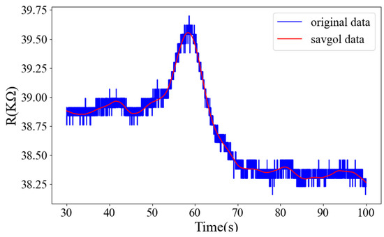
Figure 4.
Comparison diagram of gas response data curve with or without filtering.
2.4. Images Conversion
With the development of computer vision, Deep Neural Network has shown outstanding performance in image recognition. According to the time correlation embedded in the gas sensor data, the SG algorithm in the previous section is used to smooth and filter the time series data into a two-dimensional sensor image, so as to be used for the subsequent feature learning. Therefore, gas classification and recognition based on time series data are transformed into gas classification and recognition for two-dimensional sensor images. The Gramian Angular Field (GAF) method was used to convert the response data of the gas sensor into a two-dimensional sensor image. The features in the two-dimensional image were learned by combining with the gas classification network model, and the features were automatically extracted. Finally, the recognition of four gas types was realized.
The specific implementation process of Gramian Angular Field (GAF) is as follows: First, scale the sequence data of each channel in the 8-channel time series data of each test sample, of each test sample, and scale the data range to [0, 1]. The expression is as follows:, where is the normalized value at time , is the response value of the ith sensor at time , and is the response value of the ith sensor within the sampling time range. The comparison of gas response data curves with or without Savitzky–Golay smooth filtering after data normalization is shown in Figure 5a,b below.

Figure 5.
Gas response data curves: (a) without filtering after data normalization; and (b) with filtering after data normalization.
Next, the normalized time series data are converted to the polar coordinate system, that is, the value is regarded as the cosine of the included angle, and the time stamp is regarded as the radius. The formula expression is shown in (1):
Since the response data values are normalized to the interval of [0, 1], the angle range is . The polar coordinate transformation through this formula has significant advantages because the encoding is bijective, and for a given time series, the result of a given mapping in the polar coordinate system is unique. Finally, there are two methods to convert GAF image: GASF (Gramian Angular Summation Fields) and GADF (Gramian Angular Difference Fields). The formula expression is shown in (2):
For the conversion of single-channel time series gas sensing data into GAF images, GASF method was used to convert the data into two-dimensional sensing images, and the image size of single-channel two-dimensional sensing images was set to 64 × 64. The single-channel time series data are converted into a single-channel two-dimensional sensor image (including GASF and GADF methods), as shown in Figure 6 below.

Figure 6.
Single-channel 2D sensor image.
Since the gas response data of each test sample is measured by 8 gas sensors, considering that the time series data intervals intercepted by all experimental samples are identical, that is, the time column data of each sample will not affect the performance of the subsequent gas classification network model, a 3 × 3 two-dimensional combined sensor image is constructed. Finally, the gas sensor response data of each test sample are processed by GASF method and converted into a 192 × 192 two-dimensional combination sensor image. The two-dimensional combination sensor images of the four gases are shown in Figure 7 below.
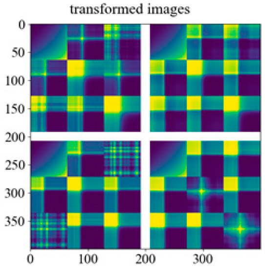
Figure 7.
The two-dimensional combination sensor images of the four gases. The x and y axis represent the number of pixels converted from the gas sensing response data to the gas sensing image.
2.5. Data Augmentation Technology
Since the collection and labeling of gas sensor array data are energy-consuming and costly processes, it is a great challenge. The total number of data samples used in this experiment is 640, and the gas recognition network model is easy to over-fit using small samples. Therefore, data augmentation technology [12] is adopted to increase the number of experimental samples, reduce the occurrence of over-fitting phenomenon, expand the decision boundary of the model, and help to improve the generalization ability of the training model, so that the gas classification model has stronger robustness. GASF method is used to convert the time series gas sensing data into two-dimensional combined sensing images. Since the Gram matrix is symmetrical about the diagonal, the sensor response image obtained is also symmetrical about the diagonal. The data augmentation technology of the experimental samples includes image mirroring, transformation brightness (brightening and darkening), and angle rotation (90° and 180°). Finally, the total amount of data samples in this experiment was increased 6 times, from 640 gas data samples to 3840 gas data samples. After that, the two-dimensional combination sensor image is input into the gas recognition network to realize the training and testing process of gas classification. The two-dimensional combined sensor image after the enhancement of single gas sample data are shown in Figure 8 below.
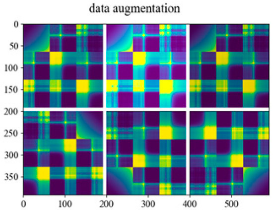
Figure 8.
A two-dimensional combined image with enhanced data from a single gas sample. The x and y axis represent the number of pixels converted from the gas sensing response data to the gas sensing image.
2.6. Model Execution
- (1)
- Introduction to the Model
Pytorch framework in deep learning is used and run on GPU to accelerate the calculation and realize the gas recognition model. The fine-tuning of GoogLeNet network structure for gas recognition is shown in Figure 9 below, which is roughly divided into five modules. The specific operation process of each module is as follows: Firstly, in the first module, a convolution layer and a maximum pooling layer are used. In our gas recognition model, the rectified linear units (ReLUs) are required after the convolution operation. In the second module, two convolution layers and one maximum pooling layer are used. Local response normalization is not adopted in the first two modules, because this layer structure does not play a significant role, so it is discarded to simplify the network model structure. In the third module, there are two layers of structure, namely inception (3a) layer and inception (3b) layer, which are divided into four branches. Multi-scale processing is adopted. Finally, the eigenmatrix of four branches of inception layer is connected in parallel to the depth direction. After that, the specific experimental operations of the fourth and fifth modules are similar to those of inception (3a) and inception (3b) in the third module. Finally, the output layer is different from the previous neural network output layer, which adopts three continuous and fully connected layers. This output layer network adopts the adaptive average pooling layer, which plays a role of dimension reduction on the one hand and abstracts the global features of the image by combining low-level features on the other hand. No matter how much the height and width of the input feature matrix are set, both the height and width of the specified feature matrix can be obtained (the convolution layer with both height and width of 1 is finally obtained), and then the dropout with 50% probability of dropping is added. Through the operation of dropout, the number of neurons and connection weights in the network will be randomly reduced, which can improve the numerical performance and prevent over-fitting. Finally, the soft-max layer (activation function) is used as the classifier to identify four different gases: methane, ethylene, ethanol, and carbon monoxide.

Figure 9.
The structure of DNN model.
GoogLeNet network model structure mainly introduces the inception architecture. The improved inception structure diagram is shown in Figure 10 below, which mainly integrates the characteristic information of different scales. On the basis of the original inception structure, a convolution layer with a convolution kernel size of 1 × 1 was added before the 3 × 3 and 5 × 5 convolution layers, and a convolution layer with a convolution kernel size of 1 × 1 was added after the pooling layer, in order to reduce the dimension and model training parameters, so as to reduce the amount of computation.
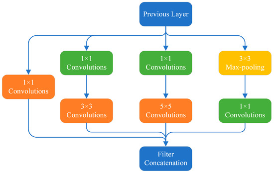
Figure 10.
Improved inception structure diagram.
- (2)
- Training and testing procedures
- 1.
- In the process of model training, Pytorch framework in deep learning is used and run on GPU to accelerate calculation and realize gas classification and recognition. In the experiment, the final goal is to classify 4 different gases. For the multi-gas classification tasks, cross-entropy loss is used as the loss function. The adaptive moment estimation (Adam) optimization algorithm is used as the optimization algorithm. Batch size is set to 32, the learning rate to 0.0003, and iterations to 100. All 2D sensing images are transformed accordingly, for example, the random aspect ratio is trimmed to 224 × 224 pixels, the horizontal flip is according to probability p = 0.5, transformed into tensors and normalized to 0~1, and the image is normalized. The gas classification is realized in combination with the fine-tuning GoogLeNet network model. It is worth noting that the two auxiliary classifiers of GoogLeNet are applied in the training of the model, the loss of the two auxiliary classifiers is multiplied by the weight and added to the overall loss of the network, and then the back propagation is carried out, which can prevent the over-fitting of the network and improve the discriminant power of the classifier at the lower network layer. In the actual test, the two auxiliary classifiers will not be used.
- (3)
- Process of prediction
In the prediction process, first load the two-dimensional sensor image after gas response data conversion. In order to match the input dimension of the network, add a Batch dimension to the prediction image. By reading the label file generated in the training process, load the model parameters saved in the training process on the basis of the model establishment, and finally realize the recognition and prediction of the image. In other words, it can accurately predict four different gases: methane, ethylene, ethanol, and carbon monoxide. The following Figure 11 shows the prediction results, achieving accurate prediction of carbon monoxide gas.
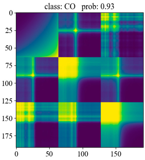
Figure 11.
Gas identification and prediction results. The x and y axis represent the number of pixels converted from the gas sensing response data to the gas sensing image.
3. Results
3.1. Basic Experiment
In the basic experiment, the Savitzky–Golay smooth filtering was carried out on the response data of the original gas sample. After that, the GASF method was used to encode the gas sensing response data into two-dimensional sensing images. In addition, data augmentation technology was also adopted in the experiment to reduce the impact of small samples on the classifier. The dataset was randomly divided into the training set and the test set according to the ratio of 8:2. Combined with the fine-tuning GoogLeNet neural network, the classification of four gases, including methane, ethanol, ethylene, and carbon monoxide, was finally realized by taking advantage of its automatic learning of deep-seated sample characteristics. As shown in Figure 12a–c, gas identification achieves a higher precision, and the convergence is completed in fewer iteration cycles and the final loss value converges to around zero. In the process of training and testing, the accuracy has the same upward trend and the two are close. In the process of training and testing, the loss value also has the same downward trend and the two are close. In addition, when the accuracy increases, the loss value shows a downward trend, indicating that there is no over-fitting phenomenon in the experimental method.

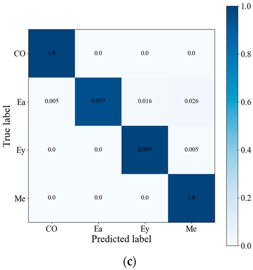
Figure 12.
(a) The training and test accuracy curves in basic experiment. (b) The training and test loss curves in basic experiment. (c) Confusion matrix of basic experiment.
3.2. Comparison Experiments
- (1)
- Influence of the 10-fold cross validation method on the experimental classification results.
In the experiment, a 10-fold cross validation method was adopted to verify the accuracy of the model recognition. The two-dimensional sensor images were divided into ten parts, nine of which were taken as training data and one as test data for experiment. As shown in Figure 13a,b, the gas recognition accuracy is 99.9%, and the gas recognition accuracy and loss rate curves in the training and testing of the model are basically the same. Despite the small oscillations during the test, the overall accuracy and loss rate curves during the training and testing process tend to smooth out and eventually stabilize. The confusion matrix of the experimental classification results is shown in Figure 13c below. It is clear from the diagram that the model performs well in identifying all four gases.

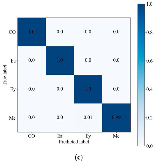
Figure 13.
(a) The training and test accuracy curves of the comparison experiment. (b) The training and test loss curves of the comparison experiment. (c) Confusion matrix of the comparison experiment.
- (2)
- The influence of smooth treatment on the experimental classification results.
In order to make the experimental research more persuasive, three smoothing filtering methods, namely Savitzky–Golay smoothing filtering, Kalman filtering, Gaussian filtering and moving average filtering, were adopted in the experiment to filter the original gas response data, respectively. The corresponding accuracy and loss rate results in the test process are shown in Table 5 below. As can be seen from Table 5, smooth filtering has well-improved the classification accuracy of the gas identification network. In particular, the Savitzky–Golay smooth filtering algorithm can better improve the accuracy of gas identification. Therefore, the subsequent comparison experiments all use the Savitzky–Golay algorithm for smooth filtering.
Table 5.
The experimental results contrast.
- (3)
- The influence of data augmentation on the experimental classification results.
In order to reduce the influence of the small sample data size of the gas sensor array on the classification network model, the data augmentation network strategy is adopted in the experiment. The data samples, with or without data augmentation, were trained and tested, respectively, in the experiment, and the number of iterations was randomly set to 200. After several experiments, it was proved that the model based on the fine-tuning GoogLeNet network structure had a fast convergence speed, and when the number of iterations was 60, it was close to convergence. Therefore, it was appropriate to set the number of iterations to 100. The experimental results of accuracy and loss rates in the testing process are shown in Figure 14a,b below. As can be seen from the figure, the gas sample data after data augmentation makes the classification model more robust, the test effect more stable, and the convergence faster, as the highest classification accuracy is 99.9%, and the loss is small. However, for the gas sample data with no data augmentation input into the classification network model, the test effect has certain data fluctuations, without good stability. The highest classification accuracy was 98.4%, and the loss was great. It can be concluded that the data augmentation network strategy can better improve the classification accuracy of the gas identification network model, so that the gas identification network model has better robustness and generalization ability.

Figure 14.
(a) Training and accuracy curves with and without data augmentation experiment. (b) Training and test loss curves with and without data augmentation experiment.
- (4)
- The influence of different sample data division ratios on the classification results.
In the experiment, the response data of gas samples were divided into different proportions of training sets and test sets. The two-dimensional sensor response image enhanced by the data in the previous section was used as the input data of the gas identification network. During the experiment, the sample data were divided into training sets and test sets according to various proportions, as shown in Table 6 below.
Table 6.
Data partition ratio.
The response data of gas samples are divided according to the division proportion of different training sets and test sets. The experimental results of the accuracy and loss rate of the test process are shown in Figure 15a,b below. In general, when dividing the gas sample data with different proportions of training set and test set, the higher the proportion of the training set data, the higher the classification accuracy will be, and the higher the proportion of the test set data, the more stable the classification results of the classifier will be.

Figure 15.
(a) Training and test accuracy curves for different proportions of divided datasets. (b) Training and test loss curves of different proportions of divided datasets.
- (5)
- The influence of different classification network models on the classification results.
The data enhanced two-dimensional sensor images were input into different classification network models for a comparison experiment. The experimental results are shown in the following Table 7. As can be seen from Table 7, the fine-tuned GoogLeNet network classification model has the highest classification accuracy, followed by the fine-tuned ResNet50 network, Alex-Net network, and finally, the ResNet34 network. In contrast, the fine-tuned GoogLeNet network classification model selected by us is more suitable for the identification of methane, ethanol, ethylene, and carbon monoxide, achieving higher recognition accuracy and more stable experimental results. The variation trends of accuracy and loss rate in the training process and the testing process are similar, which indicates that the method we adopted improves the generalization ability of the classification model.
Table 7.
Comparison of experimental results of different classification network models.
- (6)
- Compare and analyze the experimental results with others.
In order to make the experimental results more comparative and persuasive, this paper will compare them with the classification accuracy obtained by other people’s experiments on this public dataset. As can be seen from Table 8, compared with the classification accuracy achieved by other experiments in the table, our gas classification accuracy is higher, and the classification effect is better.
Table 8.
Performance of accuracy compared with other people’s experiments.
- (7)
- Application to different UCI gas datasets.
In order to apply the gas recognition algorithm proposed in this paper to the recognition of a binary gas mixture, we found the binary gas mixture dataset in the UCI machine learning library. The binary gas mixture dataset is named the gas sensor array under dynamic gas mixtures. The gas identification process uses a mixture of carbon monoxide and ethylene, and finally realizes the identification of air, carbon monoxide, ethylene, and a mixture of carbon monoxide and ethylene. Carbon monoxide ranges from 0 ppm to 533.33 ppm, and ethylene ranges from 0 ppm to 20 ppm.
The data sample processing process is as follows: when the concentration of any gas in the mixture of carbon monoxide and ethylene changes, it is divided into one data sample. Finally, it is divided into 373 binary gas data samples of four types. By using the Gramian Angular Summation Fields (GASF) method, the binary gas mixture data samples are converted into two-dimensional sensing images, and the fine-tune GoogLeNet network model is applied to the binary gas mixture image recognition, which can classify the binary gas mixture. The experimental results of the accuracy and loss rate of the test process are shown in Figure 16a,b below. It can be seen from the curve of experimental results that the gas recognition algorithm can be well applied to a binary gas mixture.
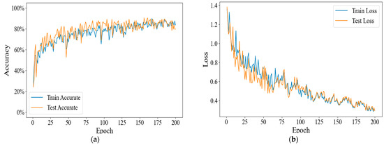
Figure 16.
(a) Training and test accuracy curves of binary gas mixture datasets. (b) Training and test loss curves of binary gas mixture datasets.
4. Discussion
As for the classification experimental results under different comparison experiments obtained in the last section, we will, respectively, discuss as follows:
(1) Firstly, the experiment adopts four different smoothing filtering algorithms to pre-process the original gas sample data. The experimental results show that, firstly, smoothing filtering pre-processing greatly improves the classification and identification accuracy of gas. The highest recognition accuracy is 99.9%. Secondly, among the smoothing filtering algorithms, the Savitzky–Golay smoothing filtering algorithm has the highest accuracy and the best effect. Compared with the other three filtering algorithms, the Savitzky–Golay smoothing filtering algorithm can better retain the information of characteristic peaks and improve the accuracy of input data. In conclusion, the smooth filtering pre-processing can filter the noise existing in the signal sample data, reduce the existence of redundant information without losing important response data information, and obtain efficient input data representation. The classification accuracy of gas verifies the superiority of the smooth filtering pre-processing method.
(2) Secondly, gas sample data collection and labeling are energy-consuming and costly processes. Data augmentation network technology is used to amplify datasets. On the one hand, the number of training samples is increased; on the other hand, the generalization ability and robustness of the model can be improved. We carried out a six-fold data enhancement on the gas sample data used in the experiment, and finally the highest classification accuracy reached 99.9%, while the highest classification accuracy of the gas sample without data enhancement was 98.4%. In addition, it can be seen from the comparison curve of the experimental results of the data classification with or without data enhancement in the previous section that the gas samples after data enhancement perform better than those without data enhancement in terms of accuracy and loss rate. The classification accuracy of gas samples with data enhancement is more stable and converges faster. Therefore, data enhancement network technology can improve the accuracy of gas classification to a certain extent.
(3) Thirdly, the gas sample data are divided into training sets and test sets according to various proportions. The higher the proportion of the training set data, the higher the classification accuracy will be; the higher the proportion of the test set data, the more stable the classification results of the classifier. Because the more training gas samples there are, the more data information they contain, the more features they will learn, and the higher classification accuracy they can achieve in subsequent tests. At the same time, setting a certain number of test gas samples of data can improve the generalization ability of the model, making the classification results more stable, preventing the occurrence of overfitting phenomenon, and finding the optimal parameters of the classification network.
(4) Fourthly, the comparison experiments of different classification networks in the previous section show that the fine-tuned GoogLeNet gas recognition network model selected is superior to the fine-tuned ResNet50, Alex-Net, and ResNet34 networks, in terms of classification accuracy, sample processing time, and network connection complexity. Since fine-tuning the GoogLeNet gas identification network model simplifies the model structure and has multi-inception structure, which can integrate feature information of different scales, two auxiliary classifiers are added to the network model to help training, and the output layer dismisses the fully connected layer and uses the average pooling layer instead, greatly reducing the model parameters. High gas classification and recognition accuracy is achieved.
(5) Finally, compared with the classification recognition accuracy of other people’s experiments on this public dataset, it was found that our experimental research achieved a higher classification accuracy. Different from other scholars’ experiments, we adopted different network strategies (data smoothing filtering and data enhancement) to efficiently optimize the input data samples and we fine-tuned the GoogLeNet gas identification network model to automatically learn subsequent features and finally achieve a higher classification accuracy.
(6) In general, we used a variety of smoothing filtering algorithms to pre-process the gas sensor data, and according to the time correlation embedded in the sensor data, we used the GASF method to convert the gas sensor data into a two-dimensional sensor image for the subsequent feature learning. We combined with the fine-tuned GoogLeNet classification network model to automatically learn the features of the sensor image to classify the four gases, and achieve a good classification accuracy.
5. Conclusions and Future Outlook
To identify different kinds of gas, we used a variety of smoothing filtering algorithms to perform data smoothing pretreatments on the multi-channel data representation and obtain efficient input data representation, improving the performance of the classification model. The optimization experiment verifies that the data from the Savitzky–Golay smoothing filtering algorithm is inputted into the gas classification network, and the final gas classification accuracy is higher. The smoothing filter pre-processing method plays a key role in the gas classification experiment, greatly improving the accuracy of the experimental results. Using the time correlation embedded in the sensor data, we used the GASF method to convert the gas sensor data into two-dimensional sensor image representations. Further gas classification is achieved using sensor images rather than time series data. Then, we also use the data enhancement network strategy to reduce the impact of small samples on the classifier, and to improve the robustness and generalization ability of the gas identification network model. The model can automatically and comprehensively extract different features of target gas for subsequent learning to realize the gas classification. Different from traditional methods, this model does not need to carry out tedious steps, such as artificial feature extraction and feature selection for gas sensing data and can directly classify the converted two-dimensional sensor image with a better classification performance. In addition, for the dataset samples in this paper, the fine-tuned GoogLeNet gas identification network model has obvious advantages over the fine-tuned ResNet50, Alex-Net, and ResNet34 networks. Compared with other advanced methods previously reported, this method has more advantages. These features help to identify gases in real time and quickly, with excellent accuracy and robustness, and they are suitable for a wide range of applications.
In our future work, we aim to find the optimal algorithm to directly classify and recognize multivariate time series data through more extensive experiments, especially on multivariate time series datasets. In addition, the time convolution neural network (TCN) and cyclic neural network (RNN) are considered to process multivariate time series data, and a variety of different classification methods are integrated to compare their classification performance. For another important future work, we hope to apply the selected method to different applications and different gas sensor array systems to further evaluate their classification performance and versatility.
Author Contributions
Conceptualization, M.J.; methodology, X.W.; software, Z.Z.; validation, C.Q. and J.L.; formal analysis, X.W.; investigation, X.W. and C.Q.; resources, M.J.; data curation, Z.Z.; writing—original draft preparation, X.W.; writing—review and editing, M.J.; visualization, X.W.; supervision, M.J.; project administration, X.W.; funding acquisition, M.J. All authors have read and agreed to the published version of the manuscript.
Funding
This research was funded by the Ministry of Science and Technology of China (2022CSJGG0703), National Natural Science Foundation of China (62204260).
Institutional Review Board Statement
Not applicable.
Informed Consent Statement
Not applicable.
Data Availability Statement
https://archive.ics.uci.edu/ml/datasets/Twin+gas+sensor+arrays (accessed on19 May 2016).
Conflicts of Interest
The authors declare no conflict of interest.
References
- Navaneeth, B.; Suchetha, M. PSO optimized 1-D CNN-SVM architecture for real-time detection and classification applications. Comput. Biol. Med. 2019, 108, 85–92. [Google Scholar] [CrossRef] [PubMed]
- Gasparri, R.; Santonico, M.; Valentini, C.; Sedda, G.; Borri, A.; Petrella, F.; Maisonneuve, P.; Pennazza, G.; D’Amico, A.; Natale, C.D. Volatile signature for the early diagnosis of lung cancer. J. Breath Res. 2016, 10, 016007. [Google Scholar] [CrossRef] [PubMed]
- Chapman, E.A.; Thomas, P.S.; Stone, E.; Lewis, C.; Yates, D.S. A breath test for malignant mesothelioma using an electronic nose. Eur. Respir. J. 2012, 40, 448–454. [Google Scholar] [CrossRef] [PubMed]
- Paknahad, M.; Ahmadi, A.; Rousseau, J.; Nejad, H.R.; Hoorfar, M. On-chip electronic nose for wine tasting: A digital microfluidic approach. IEEE Sens. J. 2017, 17, 4322–4329. [Google Scholar] [CrossRef]
- Yin, Y.; Hao, Y.; Bai, Y.; Yu, H.C. A Gaussian-based kernel Fisher discriminant analysis for electronic nose data and applications in spirit and vinegar classification. J. Food Meas. Charact. 2017, 11, 24–32. [Google Scholar] [CrossRef]
- Chen, L.Y.; Wong, D.M.; Fang, C.Y.; Chiu, C.I.; Chou, T.I.; Wu, C.C.; Chiu, S.W.; Tang, K.T. Development of an electronic-nose system for fruit maturity and quality monitoring. In Proceedings of the 2018 IEEE International Conference on Applied System Invention (ICASI), Chiba, Japan, 13–17 April 2018. [Google Scholar]
- Men, H.; Yin, C.; Shi, Y.; Liu, X.T.; Fang, H.R.; Han, X.J.; Liu, J.J. Quantification of acrylonitrile butadiene styrene odor intensity based on a novel odor assessment system with a sensor array. IEEE Access 2020, 8, 33237–33249. [Google Scholar] [CrossRef]
- Xu, L.Y.; He, J.; Duan, S.H.; Wu, X.B.; Wang, Q. Comparison of machine learning algorithms for concentration detection and prediction of formaldehyde based on electronic nose. Sens. Rev. 2016, 36, 207–216. [Google Scholar] [CrossRef]
- Liu, M.H.; Li, Y. Application of electronic nose technology in coal mine risk prediction. Chem. Eng. Trans. 2018, 68, 307–312. [Google Scholar]
- Pan, X.F.; Zhang, H.E.; Ye, W.B.; Zhao, X.J. A fast and robust gas recognition algorithm based on hybrid convolutional and recurrent neural network. IEEE Access 2019, 7, 100954–100963. [Google Scholar] [CrossRef]
- Pareek, V.; Chaudhury, S.; Singh, S. Gas Discrimination & Quantification using Sensor Array with 3D Convolution Regression Dual Network. In Proceedings of the 2021 11th IEEE International Conference on Intelligent Data Acquisition and Advanced Computing Systems: Technology and Applications (IDAACS), Cracow, Poland, 22–25 September 2021. [Google Scholar]
- Oh, Y.K.; Lim, C.; Lee, J.; Kim, S.; Kim, S. Multichannel convolution neural network for gas mixture classification. Ann. Oper. Res. 2022. [Google Scholar] [CrossRef]
- He, J.; Li, M.Y.; Zhou, R.; Li, N.; Liang, Y. Rapid Identification of Multiple Gases. In Proceedings of the 2021 3rd International Conference on Advanced Information Science and System (AISS 2021), Sanya, China, 26–28 November 2021. [Google Scholar]
- Donner, R.V.; Zou, Y.; Donges, J.F.; Marwan, N.; Kurths, J. Recurrence networks—A novel paradigm for nonlinear time series analysis. New J. Phys. 2010, 12, 033025. [Google Scholar] [CrossRef]
- Silva, D.F.; De Souza, V.M.A.; Batista, G.E.A.P.A. Time series classification using compression distance of recurrence plots. In Proceedings of the 2013 IEEE 13th International Conference on Data Mining, Dallas, TX, USA, 7–10 December 2013. [Google Scholar]
- Javed, W.; McDonnel, B.; Elmqvist, N. Graphical perception of multiple time series. IEEE Trans. Vis. Comput. Graph. 2010, 16, 927–934. [Google Scholar] [CrossRef] [PubMed]
- Wang, Z.; Oates, T. Imaging time-series to improve classification and imputation. In Proceedings of the Twenty-Fourth International Joint Conference on Artificial Intelligence, Buenos Aires, Argentina, 25–31 July 2015. [Google Scholar]
- Liu, Y.J.; Meng, Q.H.; Zhang, X.N. Data processing for multiple electronic noses using sensor response visualization. IEEE Sens. J. 2018, 18, 9360–9369. [Google Scholar] [CrossRef]
- Wang, S.H.; Chou, T.I.; Chiu, S.W.; Tang, K.T. Using a hybrid deep neural network for gas classification. IEEE Sens. J. 2020, 21, 6401–6407. [Google Scholar] [CrossRef]
- Tsui, L.; Benavidez, A.; Palanisamy, P.; Evans, L.; Garzon, F. Quantitative decoding of the response a ceramic mixed potential sensor array for engine emissions control and diagnostics. Sens. Actuators B Chem. 2017, 249, 673–684. [Google Scholar] [CrossRef]
- Yi, S.; Tian, S.; Zeng, D.; Xu, K.; Peng, X.L.; Wang, H.; Zhang, S.P.; Xie, C.S. A novel approach to fabricate metal oxide nanowire-like networks based coplanar gas sensors array for enhanced selectivity. Sens. Actuators B Chem. 2014, 204, 351–359. [Google Scholar] [CrossRef]
- Akbar, M.A.; Ali, A.A.S.; Amira, A.; Bensaali, F.; Benammar, M.; Hassan, M.; Bermak, A. An empirical study for PCA-and LDA-based feature reduction for gas identification. IEEE Sens. J. 2016, 16, 5734–5746. [Google Scholar] [CrossRef]
- Ha, D.; Ahmed, U.; Pyun, H.; Lee, C.J.; Baek, K.H.; Han, C. Multi-mode operation of principal component analysis with k-nearest neighbor algorithm to monitor compressors for liquefied natural gas mixed refrigerant processes. Comput. Chem. Eng. 2017, 106, 96–105. [Google Scholar] [CrossRef]
- Sun, J.; Xiao, Q.; Wen, J.; Wang, F. Natural gas pipeline small leakage feature extraction and recognition based on LMD envelope spectrum entropy and SVM. Measurement 2014, 55, 434–443. [Google Scholar] [CrossRef]
- Yang, F.; Zhang, L.; Yu, S.; Prokhorov, D.; Mei, X.; Ling, H. Feature pyramid and hierarchical boosting network for pavement crack detection. IEEE Trans. Intell. Transp. Syst. 2019, 21, 1525–1535. [Google Scholar] [CrossRef]
- Ahmad, F.; Abbasi, A.; Li, J.; Dobolyi, D.G.; Netemeyer, R.G.; Clifford, G.D.; Chen, H. A deep learning architecture for psychometric natural language processing. ACM Trans. Inf. Syst. (TOIS) 2020, 38, 1–29. [Google Scholar] [CrossRef]
- Mahindru, A.; Sangal, A.L. MLDroid—Framework for Android malware detection using machine learning techniques. Neural Comput. Appl. 2021, 33, 5183–5240. [Google Scholar] [CrossRef]
- Mahindru, A.; Sangal, A.L. Deepdroid: Feature selection approach to detect android malware using deep learning. In Proceedings of the 2019 IEEE 10th International Conference on Software Engineering and Service Science (ICSESS), Beijing, China, 18–20 October 2019. [Google Scholar]
- Mahindru, A.; Sangal, A.L. Perbdroid: Effective malware detection model developed using machine learning classification techniques. In A Journey towards Bio-Inspired Techniques in Software Engineering; Springer: Cham, Switzerland, 2020; pp. 103–139. [Google Scholar]
- Peng, P.; Zhao, X.J.; Pan, X.F.; Ye, W.B. Gas classification using deep convolutional neural networks. Sensors 2018, 18, 157. [Google Scholar] [CrossRef] [PubMed]
- Fonollosa, J.; Fernandez, L.; Gutiérrez-Gálvez, A.; Huerta, R.; Marco, S. Calibration transfer and drift counteraction in chemical sensor arrays using Direct Standardization. Sens. Actuators B Chem. 2016, 236, 1044–1053. [Google Scholar] [CrossRef]
- Ruijie, G. Research on Technologies of Gas Recognition by Electronic Nose Based on Deep Learning. Master’s Thesis, Computer Technology, Huazhong University of Science and Technology, Wuhan, China, 2021. [Google Scholar]


Disclaimer/Publisher’s Note: The statements, opinions and data contained in all publications are solely those of the individual author(s) and contributor(s) and not of MDPI and/or the editor(s). MDPI and/or the editor(s) disclaim responsibility for any injury to people or property resulting from any ideas, methods, instructions or products referred to in the content. |
© 2023 by the authors. Licensee MDPI, Basel, Switzerland. This article is an open access article distributed under the terms and conditions of the Creative Commons Attribution (CC BY) license (https://creativecommons.org/licenses/by/4.0/).