Abstract
The rise of gas-sensing applications and markets has led to microwave sensors associated to polymer-based sensitive materials gaining a lot of attention, as they offer the possibility to target a large variety of gases (as polymers can be easily functionalised) at ultra-low power and wirelessly (which is a major concern in the Internet of Things). A two-channel microstrip sensor with one resonator coated with 1,2 epoxybutane-functionalised poly(ethyleneimine) (EB-PEI) and the other left bare was designed and fabricated for humidity sensing. The sensor, characterised under controlled laboratory conditions, showed exponential response to RH between 0 and 100%, which is approximated to −1.88 MHz/RH% (−0.03 dB/RH%) and −8.24 MHz/RH% (−0.171 dB/RH%) in the RH ranges of 30–80% and 80–100%, respectively. This is the first reported use of EB-PEI for humidity sensing, and performances, especially at high humidity level (RH > 80%), as compared with transducer working frequencies, are better than the state of the art. When further tested in real outdoor conditions, the sensor shows satisfying performances, with 4.2 %RH mean absolute error. Most importantly, we demonstrate that the sensor is selective to relative humidity alone, irrespective of the other environmental variables acquired during the campaign (O3, NO, NO2, CO, CO2, and Temperature). The sensitivities obtained outdoors in the ranges of 50–70% and 70–100% RH (−0.61 MHz/%RH and −3.68 MHz/%RH, respectively) were close to lab results (−0.95 MHz/%RH and −3.51 MHz/%RH, respectively).
1. Introduction
Environmental, atmospheric and air quality sensors have attracted a lot of attention in recent years [1,2,3,4]. Notably, relative humidity (RH) sensors have been receiving significant attention. They are widely used in several applications such as atmospheric science [5], agriculture [6], food, environment [7], health and medical monitoring [8], etc. Typical RH sensor requirements are high sensitivity, selectivity, robustness and repeatability, fast response time, minimal cross-sensitivity to temperature and low hysteresis [9]. To achieve RH and gas sensing, optical [1], capacitive [8], resistive [10], acoustic [4,11] and microwave transducers [12,13,14] are associated with a number of materials such as metal oxides [15], polymers [16,17] and 2D materials [18]. Polymers especially offer numerous advantages over other materials for gas-sensing applications, since they can be functionalised and processed on flexible substrates. For example, in [1], authors reported a RH optical fibre loop sensor coated with a poly(vinyl alcohol) film with a sensitivity of 0.53 nm/%RH (wavelength modulation) and −0.21 dBm/%RH (intensity modulation) in a range of 40–80% RH, a temperature sensitivity of 0.0075 nm/°C and response/recovery times of 1.8 s/4 s. In the D. Chen et al. study [19], an acoustic resonator coated with poly(ethyleneimine) (PEI) nanofibers for formaldehyde vapor detection at ppb levels was developed. The proposed sensor exhibited a fast (10–25 s) response time and a reversible and linear response towards >37 ppb of formaldehyde with a sensitivity of 1.216 kHz/ppb and with a specific detection compared with other gases. Moreover, B. Chethan et al. [15] reported the humidity-sensing performance of poly(aniline)-yttrium oxide composite tested by measuring its surface resistances in the range of 11–97% RH. It showed a sensitivity of 4.5 MΩ/%RH, response/recovery times of 3 s/4 s, a 0.17% hysteresis and a limit of detection (LOD) of 1.07% RH. Poly(ethyleneimine) (PEI) has been widely used for SO2, CO2 and NO2 gas-sensing applications due to its basic chemical nature [20,21]. For instance, S. Kumar et al. [22] reported the use of PEI to functionalise a thin-film chemiresistive sensor in order to achieve a higher sensitivity of 37% of the nominal resistance (0.27 Ω/ppm) as compared with the bare sensor.
Microwave-transduction-based sensors with their high working frequency and robustness are booming, since they are suitable for noninvasive, noncontact measurements and wide applications in the Internet of Things (IoTs) [23,24]. Microwave sensors for gas monitoring are usually based on planar technologies with a resonator geometry. When associated with sensitive materials, the resonator’s electrical properties (permittivity and/or conductivity) vary in the presence of the target species. In their study, H. Yu et al. [13] proposed an ultrafast dual-band resonator humidity sensor based on belt-shaped MoO3 nanomaterial, where sensitivities of 1.93 and 2.06 MHz/%RH for 7.3 and 9.1 GHz resonance frequencies, respectively, were achieved. The designed sensor showed a 0.25% hysteresis and a response/recovery time of less than 5 s. However, the ambient conditions in which the experiment was conducted was not stated. Furthermore, various studies showed the association of polymers with microwave transducers for RH monitoring. Humidity detection with various sensitive materials such as polyimide (PI), PI–TIO2 ceramic composite and PI–AG metal composite associated to a double split-ring resonator was reported by X. Wang et al. [5]. The microwave transducer associated with PI–TiO2 exhibits the highest sensitivities of 0.88 MHz/%RH and 0.3 dB/%RH, whereas the hysteresis behaviour and the selectivity study were not described. Finally, W.T. Chen et al. [25] described an RF humidity sensor implemented with a PEI-coated microstrip resonator. The sensor showed an average sensitivity of 0.01 dB/%RH with a frequency shift of around 5 MHz for RH in a range from 0 to 100%.
In this paper, we describe a sensor with a microwave-sensing platform consisting of two microstrip interdigitated resonators printed on a flexible Kapton substrate. 1,2-epoxybutane-functionalised poly(ethyleneimine) (EB-PEI) was deposited as sensitive material to obtain a high RH sensitivity, low hysteresis and good stability. The sensitive material synthesis, the sensor design and fabrication, sensing principle, laboratory and outdoor experimental setups are described in Section 2. The experimental results and analysis of the proposed sensor are exposed in Section 3. Section 3.2 illustrates the sensor responses to RH and temperature in laboratory conditions. In Section 3.3, we present and discuss the analysis of the results obtained during the characterisation of the sensors in outdoor conditions using the Sense-City gas pollutant monitoring platform in the Paris area [26]. Two sensors (sample 1 and sample 2) with the same geometric and material characteristics were evaluated and compared. Experimental results under controlled laboratory condition show the sample 1 sensitivities in the range of 30–80% RH and 80–100% RH (1.88 MHz/RH%, −0.03 dB/RH% and −8.24 MHz/RH%, −0.171 dB/RH%, respectively). The sample 2 sensitivities were found to be −0.95 MHz/%RH and −3.51 MHz/%RH in a range of 50–70% and >70% RH, respectively. The sample 1 and 2 frequency responses were found to vary similarly and exponentially with the RH. Outdoor measurement on sample 2 revealed RH sensitivities close to lab results (−0.61 MHz/%RH and −3.68 MHz/%RH in the range of 50–70% and >70%, respectively). The prediction of the sample 2 response with calibration models using the RH only (x = RH) and all the available environment variables (x = (O3, NOx, CO, CO2, RH and Temp)) emphasised that RH is the most determining factor of the sensor response. The calibration model associated to the sensor outputs showed good performances (MAE: 4.2 %RH, Q2: 0.845) under prediction of the RH ranging from 50–95%.
2. Materials and Methods
2.1. Sensitive Material Synthesis
The gas-sensing abilities of PEI materials mostly depend on amine content, whether there are primary, secondary or tertiary amino groups. In order to better handle this parameter, and in the context of this study, we functionalised a commercial hyperbranched PEI with epoxybutane, giving rise to fully tertiary amine composed EB-PEI as shown by the scheme in Figure 1 [27]. The objective of this functionalisation was dual: making PEI materials easily processable due to the additional butane groups and adding a humidity sensitivity due to the presence of hydroxyl groups giving rise to hydrogen bonds with water. In addition, one can anticipate that the hyperbranched architecture of PEI exacerbates the sensitivity to humidity due to the higher accessibility of the hydroxyl groups.
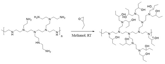
Figure 1.
Synthesis of EB-PEI from reaction of commercial PEI and epoxybutane in methanol @ RT.
2.1.1. Material and Instrumentation
Polyethyleneimine (PEI, Mw = 10 kDa) was purchased from Polysciences Inc (Warrington, PA, USA). 1,2-epoxybutane and synthesis-grade methanol were purchased from Sigma-Aldrich (St Louis, MO, USA) as received. All glassware was oven-dried prior to use. Unless otherwise stated, all starting materials and reagents were used without further purification. NMR spectra were recorded by using Bruker Avance Spectrometer (400 MHz, Bruker, Billerica, MA, USA) at room temperature (RT) in .
2.1.2. Synthesis of EB-PEI
Hyperbranched PEI (4 g, MW = 10 kDa) was dissolved in 15 mL of methanol. Afterwards, 1,2-epoxybutane (12.1 mL, equivalent to the nitrogen content of PEI) was added to the polymer solution under stirring at room temperature. After 24 h, the methanol and the unreacted epoxybutane were removed using a rotary evaporator. The product was dried in vacuum oven at 60 °C for 12 h and used for structural characterisation without further purification. Figure 2 shows the 1H-NMR (400 MHz) spectrum of EB-PEI in . 1H NMR (400 MHz, ): δ 3.54 (b, 1H), 3.44 (s, 2H), 2.70–2.53 (b, 12H), 1.39 (b, 2H), 0.93 (s, 3H). 13C NMR (150 MHz, ): 70.6, 68.9, 60.8, 53.0, 48.8, 47.1, 27.6, 10.0.
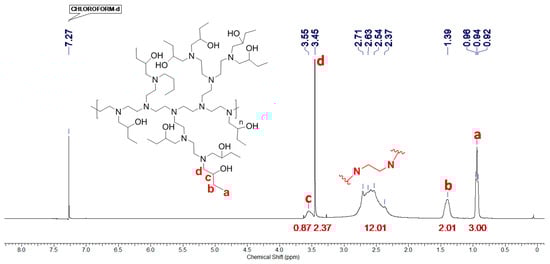
Figure 2.
1H-NMR (400 MHz) spectrum of EB-PEI in .
2.2. Microwave Resonator Design and Fabrication
The proposed microwave sensor consists of two microstrip interdigitated resonators made of 20 µm-thick copper with gold/nickel plating lines printed on a Kapton substrate, as presented in Figure 3a. The Kapton substrate is used due to its flexibility, which makes it suitable for wearable applications. One resonator is coated (sensitive channel) with the sensitive polymer layer, and the other is left bare (reference channel) in order to achieve a differential configuration. This configuration enables to minimise drifts and variations which are not induced by the sensitive materials.
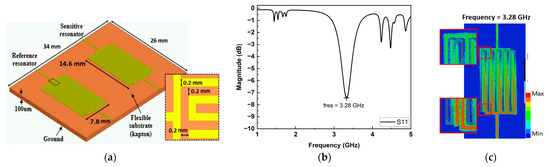
Figure 3.
Design of the microwave resonators: (a) microstrip resonators geometry, (b) simulation result of the S11 and S21 parameters of the bare resonator and (c) cartography of the electric field distribution at resonance frequency.
The sensor was designed and simulated using a 3D finite element method software (ANSYS HFSSTM) for electromagnetic circuit design. The bare resonators were designed to resonate (fres) at 3.28 GHz, as shown on Figure 3b, illustrating the reflexion (S11) scattering parameters. The resonators were optimised in order to have a maximum electric field density (cartography on Figure 3c) between the interdigitated electrodes, so as to obtain a maximum interaction of the electromagnetic wave with the sensitive material deposited [28].
The designed sensor was fabricated by BETALAYOUT [29]. Then, EB-PEI was deposited by spin coating on the sensitive channels of samples 1 and 2, as shown in Figure 4a and Figure S1a of the Supplementary Material (SM). Deposition was made on a control sample for morphological analysis. A total of 120 µm of EB-PEI was deposited on the fabricated samples, as shown on Figure 4b, illustrating the thickness measured using a numerical microscope KEYENCE VHX-500. The contact angle of the flexible Kapton substrate and EB-PEI is measured using a contact angle goniometer (Kruss, Germany), as shown in Figure S1b,c of the SM. The measured water contact angle for the Kapton substrate was found to be 34.8 ± 10.5° and that for the EB-PEI was 28.2 ± 5.3°. The hydrophilic nature of the polymer is recommended for humidity sensing, whereas that of the Kapton substrate might influence the humidity measurements. The summary of Kapton properties [30] stipulates that as RH increases the substrate dielectric constant and loss tangent increase. Moreover, the differential measurement will attenuate the effect of the variation of the substrate properties in the presence of RH.
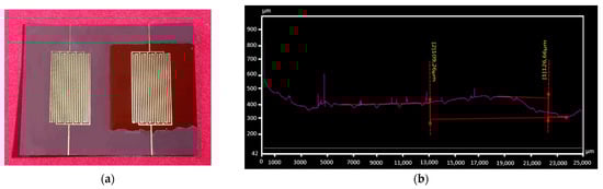
Figure 4.
(a) The fabricated sensor with EB-PEI-coated and bare resonators. (b) The measured EB-PEI thickness.
2.3. Sensing Principle
The sensing principle relies on the variation of the dielectric properties (permittivity and conductivity) of the EB-PEI in the presence of water molecules, which causes a change in the resonator scattering (S) parameters in terms of magnitude, frequency and phase. In our case, an increase in the microstrip effective permittivity due to water molecules adsorption will cause a decrease in resonance frequency as in Equation (1):
where fres is for the resonance frequency, λr is the wavelength and εeff is the effective permittivity of the microstrip line. The effective permittivity calculation of the multilayer microstrip composed of the Kapton substrate and the EB-PEI coating is given by Equation (2).
where εrsub and εrpei are the relative permittivity of the substrate and the EB-PEI, respectively. qsub and qpei are the filling factors described in [31], which are a function of the layer thickness and the microstrip line width.
On the other hand, a change in the line conductivity will lead to a change in impedance, which will cause a change in the reflection coefficient, as in Equation (3).
where Z0 is the characteristic impedance of the microstrip line. Sensing features such as magnitude (magn (dB)), frequency (freq (MHz)), phase (°) and frequency at a fixed phase (phasefreq (MHz)) are extracted from the raw S parameters spectra of the bare and coated resonators using the response extraction method described in SM, S2, Figure S2a,b.
2.4. Humidity and Temperature-Sensing Test Benches
Two test benches were used to characterise the samples under RH%, temperature and gases, as shown in Figure S3 in SM. The schematic of the experimental setup for the sensor characterisation under RH is shown in Figure 5a. It includes the sensor placed in a test cell consisting of four Sub-Miniature-A (SMA) connectors, a 4-port Vector Network Analyzer (VNA, Keysight, E5080a) controlled by Raspberry Pi 4 to measure the sensor S parameters and a commercial temperature and humidity sensor (SHT85) controlled by an Arduino Uno and a RH generator. A calibration gas generator (CALIBRAGE PUL110) is used to generate RH% in a range 0–30% at RT (20 °C), and a climatic chamber (CLIMAT) is used to generate higher RH% in a range of 30–90% at different temperatures (25–35 °C).
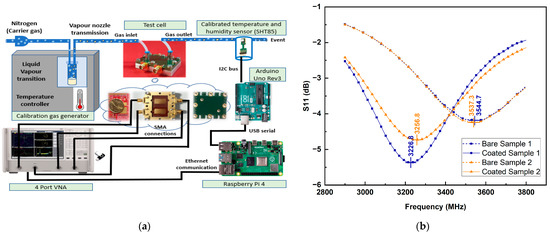
Figure 5.
(a) Schematic diagram of the experimental setup (b) Sample 1 and sample 2 experimental S11 parameters.
2.5. Performance Assessment in Environmental Conditions
In environmental conditions (e.g., outdoors), any sensor is exposed to a much larger number of varying conditions than in laboratory settings, such as ambient gas variation, rain and sun exposure. Some of these parameters may influence the sensor response, either by simply modifying the effective sensitivity of the sensor to its main target parameters, or even surpassing the nominal response. As a consequence, a wide number of studies have reported a significant lack of accuracy of environmental sensors as compared with datasheet claims [32]. To mitigate this issue, testing for all possible interfering factors in laboratory settings is feasible neither from a practical, nor from an economical perspective. A solution is to calibrate and evaluate the performances of sensors directly in environmental conditions.
This is the goal of the Sense-City (https://sense-city.ifsttar.fr/, accessed on 21 August 2021) large-scale facility. Dedicated to the full-scale validation of innovative solutions for smart cities, it incorporates all the major components of urban ecosystems (road, houses, underground networks, lightings, vegetation, etc.) which are monitored continuously with a mesh of environmental sensors. Sense-City urban scenarios are either run outdoor or within a large-scale 20 × 20 × 10 m climate chamber to test their behaviour under controlled climate conditions. To assess the sensor response in a real environment, one of the microwave sensors (sample 2) was deployed in the Sense-City facility in August 2021. The microwave sensor was connected using the setup shown in Figure S4 of SM. The sensor was placed outdoors in an alcove (to shelter it from the rain) on the side of the Sense-City climate chamber. To provide reference measurements, the environmental gas was sampled at the same location as the sensor with 1 min acquisition period, using the following analysers from Envea: AC32e for NO and NO2, O342e for N3 and CO12e for CO and CO2. The temperature and relative humidity were measured with a Vaisala WXT536 weather station located 10 m away from the sensor location.
3. Experimental Results and Discussion
3.1. Sensor Electrical Characterisation
The fabricated sensors (sample 1 and sample 2) were placed in a test cell for electrical characterisation with the VNA at ambient conditions. Figure 5b shows the S11 parameters for the bare and coated resonators of both sample 1 and sample 2. The bare and coated resonators show resonances near 3.5 GHz and 3.2 GHz, respectively. The difference with the simulated resonance frequency of 3.28 GHz for the bare sensor is mostly attributed to the test cell influence, which can be removed with appropriate de-embedding and is not expected to significantly impact the sensor’s response in terms of variations due to the target. More importantly, as seen in Figure 5b, the coated resonators show frequency shifts of −330 MHz and −300 MHz as compared with the bare resonators for samples 1 and 2, respectively. Indeed, the EB-PEI deposition causes an increase in the effective permittivity of the microstrip lines [33], thereby reducing the resonance frequency, as illustrated in Equation (1).
3.2. Sensing Performances in Lab Conditions
The sensing characteristics of the sensor to humidity were studied in laboratory conditions in a range of 0–90% RH at constant room temperature. The temperature sensitivity was also evaluated at constant RH. The sensor responses presented are given by the differential measurement between the coated resonator and the bare resonator. Frequency and phase–frequency responses being strongly correlated, only frequency responses are displayed. The sensing characteristics based on the magnitude response are given in the SM S4.
3.2.1. Humidity Response
Figure 6a displays the S11 curve of the EB-PEI-coated resonator and the influence of humidity in the range 0–90% RH. We observe a decrease in the resonance frequency and an increase in the reflection magnitude with an increase in RH. The frequency decrease with increasing RH is in agreement with an increase in the effective permittivity of the microstrip, since the water molecules are ab-/adsorbed by the sensitive polymer (Equations (1) and (2)).
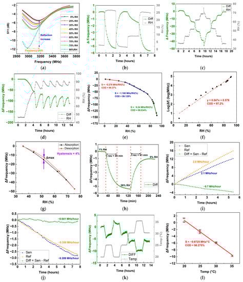
Figure 6.
Sample 1 RH and temperature-sensing performances: (a) coated resonator static frequency response when exposed to 0–90% RH, (b) dynamic differential frequency response under 0–30% RH, (c) dynamic differential frequency response under 35–75% RH, (d) dynamic differential frequency response under 80–90% RH, (e) sensor RH calibration curve of differential frequency response with its different sensitivities and CODs, (f) sensor log differential frequency response, (g) hysteresis curve of the differential frequency response in the range 35–75% RH, (h) sensor response/recovery times at 20 °C, (i) sensor desorption stabilisation when exposed to N2 at 20 °C, (j) sensor sorption drift when exposed to constant 45% RH, (k) sensor dynamic frequency response to temperature in the range 20–35 °C at 40% RH and (l) sensor temperature calibration curve with its sensitivity and COD at 40% RH.
Figure 6b–d investigate the dynamic differential frequency response of the microwave humidity sensor in the ranges 0–30% RH at RT (20 °C), 35–75% RH at 25 °C and 80–90% RH at 25 °C, respectively. In the range of 35–75% RH, a 30-min ramp was used, as shown on Figure 6c, to change the RH setpoints in order to avoid strong vibrations of the climatic chamber. The humidity level is superimposed, as monitored by the commercial sensor. We observed a clear immediate response to change in humidity, though the response time is longer. Response time is discussed in more detail in Section 3.2.2.
The calibration curve of the sensor frequency response to RH, in steady state, is represented in Figure 6e. We notice a nonlinear response to RH in the range 0–90%, the sensor being more sensitive at higher RH. The sensor exhibits the different sensitivities of −0.278 ± 0.022 MHz/%RH, −1.188 ± 0.055 MHz/%RH and −8.24 ±0.325 MHz/%RH in the ranges of 0–30% RH, 35–75% RH and 80–90% RH, respectively, as shown by the fitted lines with their corresponding coefficient of determinations (CODs) in Figure 6e. Over the whole range 0–90% RH, the frequency shift behaviour with RH can be modelled as an exponential variation: Δf = (as shown in Figure 6f). It is worth mentioning that since the Kapton substrate used in this study is slightly sensitive to RH (change in the bare resonator response, lower than the coated one—results not shown), the curve is based on the differential measurement between the EB-PEI-coated resonator and the bare resonator, in order to extract the sensor’s sensitivity due to the EB-PEI coating and not to the Kapton hydrophilicity. This reinforces the results regarding contact angle measurements reported in Section 2.2, showing that EB-PEI is more hydrophilic than the Kapton substrate.
Generally, hysteresis in RH sensor sensing is defined as the maximum difference in the response curve of the humidity sensor during humidification and dehumidification. Figure 6g shows the hysteresis characteristics and reversibility of the sensor when exposed to RH in a range 35–75%. The sensor showed a 4% hysteresis and a good reversibility.
3.2.2. Humidity Response and Recovery Times
The response time and recovery time of a sensor are defined as the time required for the sensor to reach 90% of the maximum response change in the case of the process of adsorption and desorption of the gaseous molecules, accordingly, as shown in Figure 6h. The RH variation from 1% to 26%, then down to 5%, was taken as an example, and the response/recovery times of the sensor were observed to be 45/41 min at 20 °C. The high response/recovery time observed may be partly due to the thickness of the EB-PEI coating. However, EB-PEI is not expected to be a porous polymer, and the sensing mechanism might be happening within a few top layers of the film, instead of deeply penetrating in it.
3.2.3. Sensor Long-Term Drift and Stability
Drift is an undesired feature that may be due to different factors, such as measuring instruments, sensor components, environmental factors, etc. Monotonous drift can be compensated using numerical correction methods [34], so it is not a critical challenge. Figure 6i,j, respectively, show the sensor frequency responses when exposed to a flow of dry N2 gas at 20 °C (RT) and to 45% RH at 20 °C for several hours. The former is attributed to humidity desorption stabilisation, while the latter corresponds to humidity sorption drift. Since the sensor was first under ambient conditions, the time origin on the curves is taken after waiting twice the sensor response time (90 min). The sensor shows linear curves in Figure 6i, with a 2.1 MHz/h slope for the coated resonator and 2.8 MHz/h for the bare resonator when exposed to N2 gas with a drying effect. This results in a differential response for long-term desorption of −0.7 MHz/h (which could induce an error in ambient humidity variation estimation of ~2.5 %RH/h). This long desorption stabilisation is mostly due to the hydrophilicity of the Kapton substrate itself and its low desorption time in the presence of dry N2 gas. More hydrophobic substrates should enable to reduce these effects and improve the sensor’s long-term stability. On the other hand, a linear sorption drift of −0.04 MHz/h (~0.03 %RH/h) when exposed to constant 45% RH was observed in Figure 6j, resulting from −0.39 MHz/h for the coated resonator and −0.36 MHz/h for the bare resonator. Based on these results, it appears that the differential measurement enables to reduce the nonspecific bulk effects of humidity desorption stabilisation and sorption by 66.67% and 90% for both dry N2 gas and 45% RH exposure, respectively.
3.2.4. Temperature Response and Effect on RH Sensing
RH and gas sensors should exhibit low-temperature sensitivity in order to be reliable for outdoor applications. The humidity sensor’s sensitivity to temperature is evaluated in a climatic chamber by varying temperature in the range from 20 °C to 35 °C and setting RH to 40%. Figure 6k shows the sensor dynamic differential frequency response to temperature steps. Changing the temperature setpoint causes an abrupt slight change in RH, which introduces a peak in the sensor response (~1 MHz) at each step transition. The sensor recorded a linear temperature sensitivity of −0.676 MHz/°C, as shown on the calibration curve in Figure 6l. Temperature causes a variation in the microstrip line impedance and electrical properties of the sensitive material, resulting in a shift in resonance frequency. The variation observed (decrease in resonance frequency with temperature) is compatible with an increase in permittivity of the EB-PEI and/or dilation of the polymer (increase in thickness) with temperature, leading to an increase in effective permittivity. Indeed, epoxy–hyperbranched PEIs are known to have three relaxations γ, β and α, attributed to motion of terminal end groups, motion of branches and existence of ionic charges within the PEI network, respectively. Out of these, α relaxation, associated with the glass transition of the material, appears between 0 to 60 °C, which is the similar temperature window observed in our case. So, it is possible that dilation could be one of the reasons for variation of effective permittivity within the given temperature range [35]. The effect of temperature on the sensor response to humidity is illustrated in Figure 7a. The response time is calculated after the end of the 30-min ramp (black dash dot line) used to change the RH setpoint. Increasing the temperature reduces the sensor response time quite linearly over this small temperature range, as shown by Figure 7b: tres(min) = (−2.51 ± 0.10) *T (°C) + 94.7 ± 2.7.
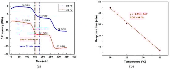
Figure 7.
Effect of temperature on the sensor RH response: (a) dynamic frequency variation with steps of RH at 25 and 35 °C; (b) response time vs. temperature.
3.2.5. Sensor Repeatability and Reproducibility
The sensor repeatability was evaluated by repeating the RH sensing experiments several times. A good repeatability with a standard deviation of 6 MHz was observed. To estimate the sensor reproducibility, the entire RH characterisation experiment was reproduced with sample 2. Figure 8a,b shows the dynamic frequency response and the RH calibration curve of sample 2 when exposed to RH in a range of 30–90% RH. Figure 8c highlights a good accordance between the RH sensitivity of sample 1 and sample 2. We observe that the sensors exhibit a good reproducibility, the frequency response of both samples varies exponentially, with RH following the laws in Figure 8c.
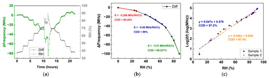
Figure 8.
Sample 2 RH characterisation: (a) dynamic frequency response in the range 35–75% RH, (b) RH calibration curve with its different sensitivities and CODs and (c) steady-state frequency response to RH and comparison with sample 1.
3.2.6. Comparison with the Literature
Table 1 synthesises microwave humidity sensors with different geometries based on various sensitive materials in terms of: sensitivity in frequency and magnitude, RH range, hysteresis, fabrication technic and operation frequency. The LOD was not reported as not specified in the articles. The sensor proposed in this work appears as a good compromise, offering advantages in terms of collective fabrication on flexible substrate and a good sensitivity in frequency and magnitude, especially for high humidity levels (RH > 80%), as compared with the working frequencies.

Table 1.
Comparison of microwave humidity sensors based on different sensitive materials.
3.3. Humidity-Sensing Performances in Environmental Conditions
3.3.1. Description of Sensor Response in Outdoor Conditions
In this section, we study how the sensor sensitivity to humidity as experimented under laboratory conditions transfers to a real environment. Figure 9 shows the six environmental parameters and Figure 10 the four differential outputs (Sen–Ref) obtained from the sensor (sample 2) measured from 26 August to 2 September 2021 at Sense-City. The data acquisition time was 40 s and is the reference for the time index.
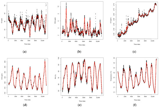
Figure 9.
Environmental parameters measured in Sense-City: (a) O3 (ppb), (b) NOx (ppb) (c) CO (ppm), (d) CO2 (ppm), (e) RH (%) and (f) Temperature (°C). The black and red lines show the raw and filtered data respectively.
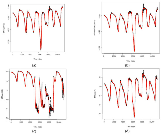
Figure 10.
Sensor differential outputs (a) ΔFreq, (b) ΔPhasefreq, (c) ΔMagn and (d) ΔPhase. The black and red lines show the raw and filtered data respectively.
The output entitled ∆Magn (Figure 10c) is particularly noisy between day 4 and 6, and was thus discarded from the rest of the analysis. A denoising procedure based on a noisy Gaussian process regression model was then applied to smooth the measured data, followed by a normalisation step to avoid scaling effects (subtraction of the mean value and division by the standard deviation) [42].
The daily cycles are obvious for O3, CO2, RH and Temperature, as well as the sensor’s parameters, but not for NOx (the sum of NO2 and NO mass concentrations) nor CO. As a first analysis, the linear correlation between the nine parameters (three outputs and six inputs) is displayed in Figure 11: the value 1 (resp. the value −1) shows a perfect positive (resp. negative) linear correlation between two parameters, while 0 indicates the absence of linear correlation.
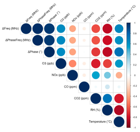
Figure 11.
Correlation analysis.
A strong correlation between the three sensors’ outputs can first be noticed, which is confirmed when applying a PCA (principal component analysis) on these three parameters: most of the signal’s energy (around 85%) appears to be carried by the first principal component, which is close to the average of the three signals, and the second component only brings 10% of the remaining energy. In the further analysis, considering the closeness between the three signals, only images regarding the “frequency” parameter are displayed (the illustrations associated with the two other outputs are displayed in SM S5).
The strongest correlation between sensor outputs and environmental parameters is found to be with relative humidity. Weaker correlations are found with temperature, O3, CO2 and NOx, and there is no correlation with CO. This is in agreement with a strong correlation between all the environmental parameters except CO and can be explained by the presence of ozone and NOX that is strongly related to sunshine, as are temperature and humidity. It, however, complicates the performance analysis of the sensors studied: if the sensor is sensitive to one of these environmental variables, it also becomes indirectly sensitive to all the intercorrelated ones.
To confirm the capability of the proposed sensor to serve as humidity sensor in the field conditions, we built a calibration model for humidity (Section 3.3.2), then used it to predict humidity (Section 3.3.3). We also studied the influence of the other environmental parameters on calibration and prediction.
3.3.2. Construction of the Calibration Model for Relative Humidity
Calibration models provide the relationship x → yi(x) between each of the three sensors outputs yi, 1 ≤ i ≤ 3 and the vector x of the input variables of interest. Based on the previous results, two sets of models were investigated, those including RH (x = RH) only and those including all the environment variables (x = (O3, NOx, CO, CO2, RH and Temp)). The models were approximated using Gaussian process regression (including an additive error model), as described in [42]. The training dataset was composed of day 2 and day 3.
Figure 12 shows the results: overall, the predictive capability of the model is good, with a coefficient of determination over the testing/prediction phase Q2 of 0.87 when considering the humidity alone and 0.88 with all the environment variables. Interestingly, accounting for additional variables in the model does not much improve the mean prediction performances (almost the same Q2 value). It reinforces the results of the previous section, where humidity is found to be the most determining factor to the sensor’s response.
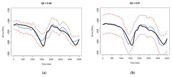
Figure 12.
Prediction of output ΔFreq using a calibration model accounting either for all the environment variables (a) or for RH only (b). Q2 is the coefficient of determination over the prediction phase. The thick black line is the sensor output, the thin blue solid line is the mean prediction of the sensor output using the calibration model learnt over the training phase and the red dotted lines are the upper and lower bounds of the 95% prediction intervals.
For both models, while the true value of the three outputs falls quasi-systematically within the 95% prediction interval, there are significant discrepancies around the extrema of the signals. The most likely explanation for the errors in peak values is the long response time of the sensors, which tends to dampen the sensor responses at the extrema of the environmental variables. The errors observed in peak values are not suppressed by accounting for the other environmental factors, but the prediction uncertainties seem to be slightly better fitted in that case.
3.3.3. Humidity Prediction
Using the calibration relationship discussed above, the value of humidity can then be predicted over the testing set (day 2 and day 3) with only the knowledge of the calibration relationship over the training set and the three outputs of the sensor. The result is shown in Figure 13a. The mean absolute error (MAE) is found to be as low as 4.2% for RH ranging from 50% to 95%, with Q² = 0.845. This shows undoubtedly the capability of the proposed sensor to measure humidity in a real environment, despite the presence of various interfering environmental factors.
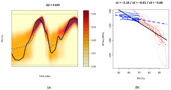
Figure 13.
(a) Prediction of RH using the sensor outputs only and the calibration relationship previously learnt. The black solid line is the measure of RH, and the blue dotted line indicates the mean prediction. The coloured areas indicate the most likely RH values: the closer to dark red, the more likely (according to the calibration relationship) the RH value is in these areas. (b) ΔFreq versus RH (%) over 7 days. The blue (resp. red) line corresponds to data below (resp. above) 70%. The blue (resp. red) dashed line shows the best linear regression fitting the data below (resp. above) 70% RH, with s2 (resp. s3) as the corresponding sensitivity (in MHz/%). The black line shows the regression for the full dataset (with s1 as the corresponding sensitivity).
Analysing the results further, the colour code in Figure 13a shows the probability distribution function (PDF) of RH values around their mean prediction marked by the blue dotted line. The PDF, however, indicates a large uncertainty for the prediction, especially for the low values of RH. This is attributed to the fact that the sensitivity to RH is higher (−3.68 MHz/%RH) at higher RH values (>70%) than at lower ones (−0.61 MHz/%RH), as confirmed in Figure 13b. Interestingly, these sensitivity values are close to lab results: −3.51 MHz/%RH above 70% RH and −0.95 MHz/%RH between 50% and 70% RH.
Finally, we carried out calibration with RH and each of the other additional environmental parameters (separately), then we predicted RH knowing the sensor outputs and the other additional environmental parameter. The goal was to determine whether there was any other environmental parameter influencing the sensor beside RH. Particularly, based on lab data, one expected an influence of temperature. Interestingly, we observed no improvement in the RH prediction when adding knowledge of any of the other environment variables. This means that the sensor does not suffer significant interferences in real conditions, which is an exceptional result.
4. Conclusions
In this paper, a microwave transducer associated with the EB-PEI polymer material evaluated under controlled and in real outdoor conditions for selective humidity detection was presented. The sensor evaluated under controlled laboratory conditions showed exponential sensitivity to RH between 0 and 100%. This is the first reported use of EB-PEI for humidity sensing, and performances, especially at high humidity level (RH > 80%), as compared with the transducer working frequencies, are better than the state of the art. The sensitivities obtained outdoors in the ranges of 50–70% and 70–100% RH were close to lab results. Furthermore, by using a performant calibration model, the overall results demonstrate the sensor’s ability to predict relative humidity under real outdoor conditions with very little interference from other environmental variables, including temperature. The limitation of outdoor measurements is the short duration of measurement, which leads to a strong correlation (seasonal/weather) between environmental variables, which complicates their decorrelation. In the future, a longer exposure to outdoor environmental conditions will be conducted in order to obtain more data, allowing the decorrelation of these climate-related parameters.
Supplementary Materials
The following supporting information can be downloaded at: https://www.mdpi.com/article/10.3390/chemosensors11010016/s1, Figure S1. Fabricated sensor and water contact angle measurements. Figure S2. Sensor response extraction algorithm. Figure S3. Laboratory experimental setups. Figure S4. Outdoor experimental setup. Figure S5. Sensor magnitude response to RH in range 0–90%. Figure S6. Sensor long-term stability and response and recovery time extracted from magnitude response. Figure S7. Sensor magnitude response to temperature. Figure S8. Variance-based sensitivity analysis in environmental conditions.
Author Contributions
B.B.N., H.H., B.L., G.P., C.D. and E.C. conceived the study and wrote the manuscript, and all authors revised the manuscript. J.G., with the supervision of S.B. and D.B., designed and performed the RF structure simulation and hyperfrequency measurements after fabrication. E.C. and S.S. synthesised the sensitive polymer material and provided the materials and structural analyses. B.B.N., H.H. and C.D. conducted the measurements under controlled environment and the results analysis. B.B.N., B.L. and G.P. realised the experiment in outdoor conditions and developed the corresponding algorithms for data exploitation. All authors have read and agreed to the published version of the manuscript.
Funding
This work was carried out with the financial support of the Agence Nationale de la Recherche (ANR) for projects CARDIF (ANR-19-CE04-0010) and CAMUS (ANR-13-BS03-0010), and of the French region Nouvelle-Aquitaine and ISORG (project CARGESE, 2017-1R10123).
Institutional Review Board Statement
Not applicable.
Informed Consent Statement
Not applicable.
Data Availability Statement
Data available upon request.
Acknowledgments
B.L et G.P. thank Stéphane Laporte and Yan Ulanowski for their support regarding the outdoor experiment in Sense-City.
Conflicts of Interest
The authors declare no conflict of interest. The funders had no role in the design of the study; in the collection, analyses, or interpretation of data; in the writing of the manuscript; or in the decision to publish the results.
References
- Sun, D.; Chen, J.; Fu, Y.; Ma, J. A real-time response relative humidity sensor based on a loop microfiber coated with polyvinyl alcohol film. Measurement 2022, 187, 110359. [Google Scholar] [CrossRef]
- Zhang, J.; Ma, S.; Wang, B.; Pei, S. Hydrothermal synthesis of SnO2-CuO composite nanoparticles as a fast-response ethanol gas sensor. J. Alloys Compd. 2021, 886, 161299. [Google Scholar] [CrossRef]
- He, Q.; Wang, Z.; Li, J. Application of the Deep Neural Network in Retrieving the Atmospheric Temperature and Humidity Profiles from the Microwave Humidity and Temperature Sounder Onboard the Feng-Yun-3 Satellite. Sensors 2021, 21, 4673. [Google Scholar] [CrossRef] [PubMed]
- Fauzi, F.; Rianjanu, A.; Santoso, I.; Triyana, K. Gas and humidity sensing with quartz crystal microbalance (QCM) coated with graphene-based materials—A mini review. Sens. Actuators A Phys. 2021, 330, 112837. [Google Scholar] [CrossRef]
- Wang, X.; Liang, J.-G.; Wu, J.-K.; Gu, X.-F.; Kim, N.-Y. Microwave detection with various sensitive materials for humidity sensing. Sens. Actuators B Chem. 2022, 351, 130935. [Google Scholar] [CrossRef]
- Owji, E.; Mokhtari, H.; Ostovari, F.; Darazereshki, B.; Shakiba, N. 2D materials coated on etched optical fibers as humidity sensor. Sci Rep 2021, 11, 1771. [Google Scholar] [CrossRef]
- Hallil, H.; Heidari, H. Smart Sensors for Environmental and Medical Applications; John Wiley & Sons: Hoboken, NJ, USA, 2020. [Google Scholar]
- Wang, Y.; Zhang, L.; Zhang, Z.; Sun, P.; Chen, H. High-Sensitivity Wearable and Flexible Humidity Sensor Based on Graphene Oxide/Non-Woven Fabric for Respiration Monitoring. Langmuir 2020, 36, 9443–9448. [Google Scholar] [CrossRef]
- Haick, H.; Tang, N. Artificial Intelligence in Medical Sensors for Clinical Decisions. ACS Nano 2021, 15, 3557–3567. [Google Scholar] [CrossRef]
- Wu, W.; Haick, H. Materials and Wearable Devices for Autonomous Monitoring of Physiological Markers. Adv. Mater. 2018, 30, e1705024. [Google Scholar] [CrossRef]
- Nikolaou, I.; Hallil, H.; Conedera, V.; Deligeorgis, G.; Dejous, C.; Rebiere, D. Inkjet-Printed Graphene Oxide Thin Layers on Love Wave Devices for Humidity and Vapor Detection. IEEE Sens. J. 2016, 16, 7620–7627. [Google Scholar] [CrossRef]
- Yu, H.; Wang, C.; Meng, F.; Xiao, J.; Liang, J.; Kim, H.; Bae, S.; Zou, D.; Kim, E.-S.; Kim, N.-Y.; et al. Microwave humidity sensor based on carbon dots-decorated MOF-derived porous Co3O4 for breath monitoring and finger moisture detection. Carbon 2021, 183, 578–589. [Google Scholar] [CrossRef]
- Yu, H.; Wang, C.; Meng, F.-Y.; Liang, J.-G.; Kashan, H.S.; Adhikari, K.K.; Wang, L.; Kim, E.-S.; Kim, N.-Y. Design and analysis of ultrafast and high-sensitivity microwave transduction humidity sensor based on belt-shaped MoO3 nanomaterial. Sens. Actuators B Chem. 2020, 304, 127138. [Google Scholar] [CrossRef]
- Hallil, H.; Ménini, P.; Aubert, H. Novel Microwave Gas Sensor using Dielectric Resonator With SnO2 Sensitive Layer. Procedia Chem. 2009, 1, 935–938. [Google Scholar] [CrossRef]
- Chethan, B.; Raj Prakash, H.G.; Ravikiran, Y.T.; Vijaya Kumari, S.C.; Manjunatha, S.; Thomas, S. Humidity sensing performance of hybrid nanorods of polyaniline-Yttrium oxide composite prepared by mechanical mixing method. Talanta 2020, 215, 120906. [Google Scholar] [CrossRef] [PubMed]
- Jang, C.; Park, J.K.; Yun, G.H.; Choi, H.H.; Lee, H.J.; Yook, J.G. Radio-Frequency/Microwave Gas Sensors Using Conducting Polymer. Materials 2020, 13, 2859. [Google Scholar] [CrossRef]
- Kang, T.-G.; Park, J.-K.; Yun, G.-H.; Choi, H.H.; Lee, H.-J.; Yook, J.-G. A real-time humidity sensor based on a microwave oscillator with conducting polymer PEDOT:PSS film. Sens. Actuators B Chem. 2019, 282, 145–151. [Google Scholar] [CrossRef]
- Bahoumina, P.; Hallil, H.; Lachaud, J.L.; Abdelghani, A.; Frigui, K.; Bila, S.; Baillargeat, D.; Ravichandran, A.; Coquet, P.; Paragua, C.; et al. Microwave flexible gas sensor based on polymer multi wall carbon nanotubes sensitive layer. Sens. Actuators B Chem. 2017, 249, 708–714. [Google Scholar] [CrossRef]
- Chen, D.; Yang, L.; Yu, W.; Wu, M.; Wang, W.; Wang, H. Micro-Electromechanical Acoustic Resonator Coated with Polyethyleneimine Nanofibers for the Detection of Formaldehyde Vapor. Micromachines 2018, 9, 62. [Google Scholar] [CrossRef]
- Cho, S.Y.; Cho, K.M.; Chong, S.; Park, K.; Kim, S.; Kang, H.; Kim, S.J.; Kwak, G.; Kim, J.; Jung, H.T. Rational Design of Aminopolymer for Selective Discrimination of Acidic Air Pollutants. ACS Sens. 2018, 3, 1329–1337. [Google Scholar] [CrossRef]
- Barauskas, D.; Pelenis, D.; Vanagas, G.; Viržonis, D.; Baltrušaitis, J. Methylated poly (Ethylene) imine modified capacitive micromachined ultrasonic transducer for measurements of CO2 and SO2 in their mixtures. Sensors 2019, 19, 3236. [Google Scholar] [CrossRef]
- Kumar, S.; Pavelyev, V.; Mishra, P.; Tripathi, N. Thin film chemiresistive gas sensor on single-walled carbon nanotubes-functionalized with polyethylenimine (PEI) for NO2 gas sensing. Bull. Mater. Sci. 2020, 43, 61. [Google Scholar] [CrossRef]
- Hallil, H.; Dejous, C.; Hage-Ali, S.; Elmazria, O.; Rossignol, J.; Stuerga, D.; Talbi, A.; Mazzamurro, A.; Joubert, P.-Y.; Lefeuvre, E. Passive Resonant Sensors: Trends and Future Prospects. IEEE Sens. J. 2021, 21, 12618–12632. [Google Scholar] [CrossRef]
- Gugliandolo, G.; Naishadham, K.; Neri, G.; Fernicola, V.C.; Donato, N. A Novel Sensor-Integrated Aperture Coupled Microwave Patch Resonator for Humidity Detection. IEEE Trans. Instrum. Meas. 2021, 70, 9506611. [Google Scholar] [CrossRef]
- Chen, W.T.; Mansour, R.R. RF Humidity Sensor Implemented with PEI-Coated Compact Microstrip Resonant Cell. In Proceedings of the 2017 IEEE MTT-S International Microwave Workshop Series on Advanced Materials and Processes for RF and THz Applications (IMWS-AMP), Pavia, Italy, 20–22 September 2017. [Google Scholar]
- Sense-City Plateform for Realtime Atmospheric Condition Simulation and Mesurement. Available online: https://sense-city.ifsttar.fr/ (accessed on 21 August 2021).
- Kim, C.; Choi, W.; Choi, M. SO2-Resistant Amine-Containing CO2 Adsorbent with a Surface Protection Layer. ACS Appl Mater Interfaces 2019, 11, 16586–16593. [Google Scholar] [CrossRef] [PubMed]
- Hallil, H.; Bahoumina, P.; Pieper, K.; Lachaud, J.L.; Rebière, D.; Abdelghani, A.; Frigui, K.; Bila, S.; Baillargeat, D.; Zhang, Q. Differential passive microwave planar resonator-based sensor for chemical particle detection in polluted environments. IEEE Sens. J. 2018, 19, 1346–1353. [Google Scholar] [CrossRef]
- PCB Manufacturer from Germany. Available online: https://eu.beta-layout.com/ (accessed on 11 June 2021).
- Summary of Kapton Properties. Available online: https://www.dupont.com/content/dam/dupont/amer/us/en/products/ei-transformation/documents/EI-10142_Kapton-Summary-of-Properties.pdf (accessed on 11 June 2021).
- Svacina, J. A simple quasi-static determination of basic parameters of multilayer microstrip and coplanar waveguide. IEEE Microw. Guid. Wave Lett. 1992, 2, 385–387. [Google Scholar] [CrossRef]
- Karagulian, F.; Barbiere, M.; Kotsev, A.; Spinelle, L.; Gerboles, M.; Lagler, F.; Redon, N.; Crunaire, S.; Borowiak, A. Review of the Performance of Low-Cost Sensors for Air Quality Monitoring. Atmosphere 2019, 10, 506. [Google Scholar] [CrossRef]
- Ramos, A.; Girbau, D.; Lazaro, A.; Villarino, R. Wireless Concrete Mixture Composition Sensor Based on Time-Coded UWB RFID. IEEE Microw. Wirel. Compon. Lett. 2015, 25, 681–683. [Google Scholar] [CrossRef]
- Di Carlo, S.; Falasconi, M. Drift Correction Methods for Gas Chemical Sensors in Artificial Olfaction Systems: Techniques and Challenges; INTECH Open Access Publisher: London, UK, 2012. [Google Scholar]
- Roman, F.; Colomer, P.; Calventus, Y.; Hutchinson, J.M. Study of Hyperbranched Poly(ethyleneimine) Polymers of Different Molecular Weight and Their Interaction with Epoxy Resin. Materials 2018, 11, 410. [Google Scholar] [CrossRef]
- Park, J.K.; Kang, T.G.; Kim, B.H.; Lee, H.J.; Choi, H.H.; Yook, J.G. Real-time Humidity Sensor Based on Microwave Resonator Coupled with PEDOT:PSS Conducting Polymer Film. Sci. Rep. 2018, 8, 439. [Google Scholar] [CrossRef]
- Kim, Y.-H.; Jang, K.; Yoon, Y.J.; Kim, Y.-J. A novel relative humidity sensor based on microwave resonators and a customized polymeric film. Sens. Actuators B Chem. 2006, 117, 315–322. [Google Scholar] [CrossRef]
- Chen, C.-M.; Xu, J.; Yao, Y. Fabrication of miniaturized CSRR-loaded HMSIW humidity sensors with high sensitivity and ultra-low humidity hysteresis. Sens. Actuators B: Chem. 2018, 256, 1100–1106. [Google Scholar] [CrossRef]
- Liu, Y.; Huang, H.; Wang, L.; Cai, D.; Liu, B.; Wang, D.; Li, Q.; Wang, T. Electrospun CeO 2 nanoparticles/PVP nanofibers based high-frequency surface acoustic wave humidity sensor. Sens. Actuators B Chem. 2016, 223, 730–737. [Google Scholar] [CrossRef]
- Li, R.-Z.; Ji, J.; Liu, L.; Wu, Z.; Ding, D.; Yin, X.; Yu, Y.; Yan, J. A high-sensitive microwave humidity sensor based on one-step laser direct writing of dielectric silver nanoplates. Sens. Actuators B Chem. 2022, 370, 132455. [Google Scholar] [CrossRef]
- Amin, E.M.; Karmakar, N.C.; Winther-Jensen, B. Polyvinyl-alcohol (PVA)-based RF humidity sensor in microwave frequency. Prog. Electromagn. Res. B 2013, 54, 149–166. [Google Scholar] [CrossRef]
- Santner, T.B.W.; Notz, W.; Williams, B. The Design and Analysis of Computer Experiments; Springer: Berlin/Heidelberg, Germany, 2003. [Google Scholar]


Disclaimer/Publisher’s Note: The statements, opinions and data contained in all publications are solely those of the individual author(s) and contributor(s) and not of MDPI and/or the editor(s). MDPI and/or the editor(s) disclaim responsibility for any injury to people or property resulting from any ideas, methods, instructions or products referred to in the content. |
© 2022 by the authors. Licensee MDPI, Basel, Switzerland. This article is an open access article distributed under the terms and conditions of the Creative Commons Attribution (CC BY) license (https://creativecommons.org/licenses/by/4.0/).