Monitoring of MSW Incinerator Leachate Using Electronic Nose Combined with Manifold Learning and Ensemble Methods

Abstract

Waste incineration is regarded as an ideal method for municipal solid waste disposal (MSW), with the advantages of waste-to-energy, lower secondary pollution, and greenhouse gas emission mitigation. For incineration leachate, the information from the headspace gas that varies at different processing processes and might be useful for chemical analysis, is ignored. The study applied a novel electronic nose (EN) to mine the information from leachate headspace gas. By combining manifold learnings (principal component analysis (PCA) and isometric feature mapping (ISOMAP), and uniform manifold approximation and projection (UMAP) and ensemble techniques (light gradient boosting machine (lightGBM) and extreme gradient boosting (XGBT)), EN based on the UMAP-XGBT model had the best classification performance with a 99.95% accuracy rate in the training set and a 95.83% accuracy rate in the testing set. The UMAP-XGBT model showed the best prediction ability for leachate chemical parameters (pH, chemical oxygen demand, biochemical oxygen demand, ammonia, and total phosphorus), with R² higher than 0.99 both in the training and testing sets. This is the first study of the EN application for leachate monitoring, offering an easier and quicker detection method than traditional instrumental measurements for the enforcement and implementation of effective monitoring programs.

1. Introduction

The world generates 2.01 billion tons of municipal solid waste (MSW) annually, and waste generated per person per day averages at 0.74 kg. When looking forward, global waste is expected to grow to 3.40 billion tons by 2050 [1]. Comprised of physicochemical and biological characteristics that are aggressive to the soil, water resources, fauna and flora, and MSW is difficult to handle for most countries and regions [2]. To date, the main disposal methods for MSW are landfill and incineration. MSW landfill causes some issues to the environment, including: (1) high greenhouse gas (GHG) emissions if landfill gas is not properly collected, (2) leachate produced damages the ecosystem, (3) a larger space is needed for the project set up [3]. Therefore, waste incineration is regarded as an ideal method for MSW disposal [4], with the advantages of waste-to-energy, lower secondary pollution, greenhouse gas emission mitigation, and so on.

However, for MSW incineration, a considerable number of challenges are still generated at different points, including but not limited to leachate processing. For incineration leachate, research has mainly focused on the characteristics of leachate concentrate [5], the organic matter molecular transformation in leachate [6], and the degradation of refractory organics [7]. All these direct or indirect studies relate to the leachate headspace gas, which hints that the information in the leachate headspace gas can be mined for leachate processing or monitoring. Until now, few in-depth studies have been conducted to fetch information from the vast amounts of original data about the varieties, concentrates, and changes of those materials.

The electronic nose (EN) appears to be a promising candidate for headspace gas detecting, mimicking the human nose, with a range of applications, including the food industry, disease diagnosis, and environment monitoring [8]. Different from instrumental methods, such as gas chromatography (GC) with a flame photometric detector (FID), photoionization (PID), or a mass spectrometer (MS), EN offers the whole information that is unique for each sample headspace gas instead of specific materials or their concentrations. EN has been predominately used for indoor air monitoring [9], soil contamination detection [10], and water quality monitoring [11]. However, studies on leachate detection based on EN technology are rare, according to our best knowledge.

Novel EN devices, based on machine learning algorithms capable of real-time detection of industrial and municipal pollutants, have been developed to monitor specific environmental-pollutant levels for enforcement and implementing effective pollution-abatement programs [12]. Manifold learning, such as isometric feature maps (ISOMAPs) and uniform manifold approximation and projection (UMAP), uncover a low-dimensional manifold embedded in a high-dimensional space while respecting the intrinsic geometry [13]. Manifold learning, as a novel data pre-processing technology, can improve the performance of EN detecting.

Ensemble methods are designed to overcome problems with weak predictors and meet the fast, high-performance requirement [14]. Combining manifold learning and ensemble methods techniques makes it possible to identify and differentiate between gases of different leachate samples based on EN and mine useful information for leachate monitoring. A novel EN based on manifold learning and ensemble methods was applied to monitor the changes in leachate headspace gas. The main objectives are: (1) to study the variation of leachate headspace gas based on EN with different processing procedures; (2) to investigate the manifold structure of EN original data based on principal component analysis, ISOMAP, and UMAP; and (3) to mine the relationship between leachate headspace gas and chemical parameter changes based on ensemble methods (extreme gradient boosting and light gradient boosting machines). The study provides insights into the relationship between leachate gas emission and chemical parameters based on EN combined with manifold learning and ensemble methods and offers an easier and quicker monitoring method than traditional instrumental measurements for the enforcement and implementation of effective monitoring programs.

2. Materials and Methods

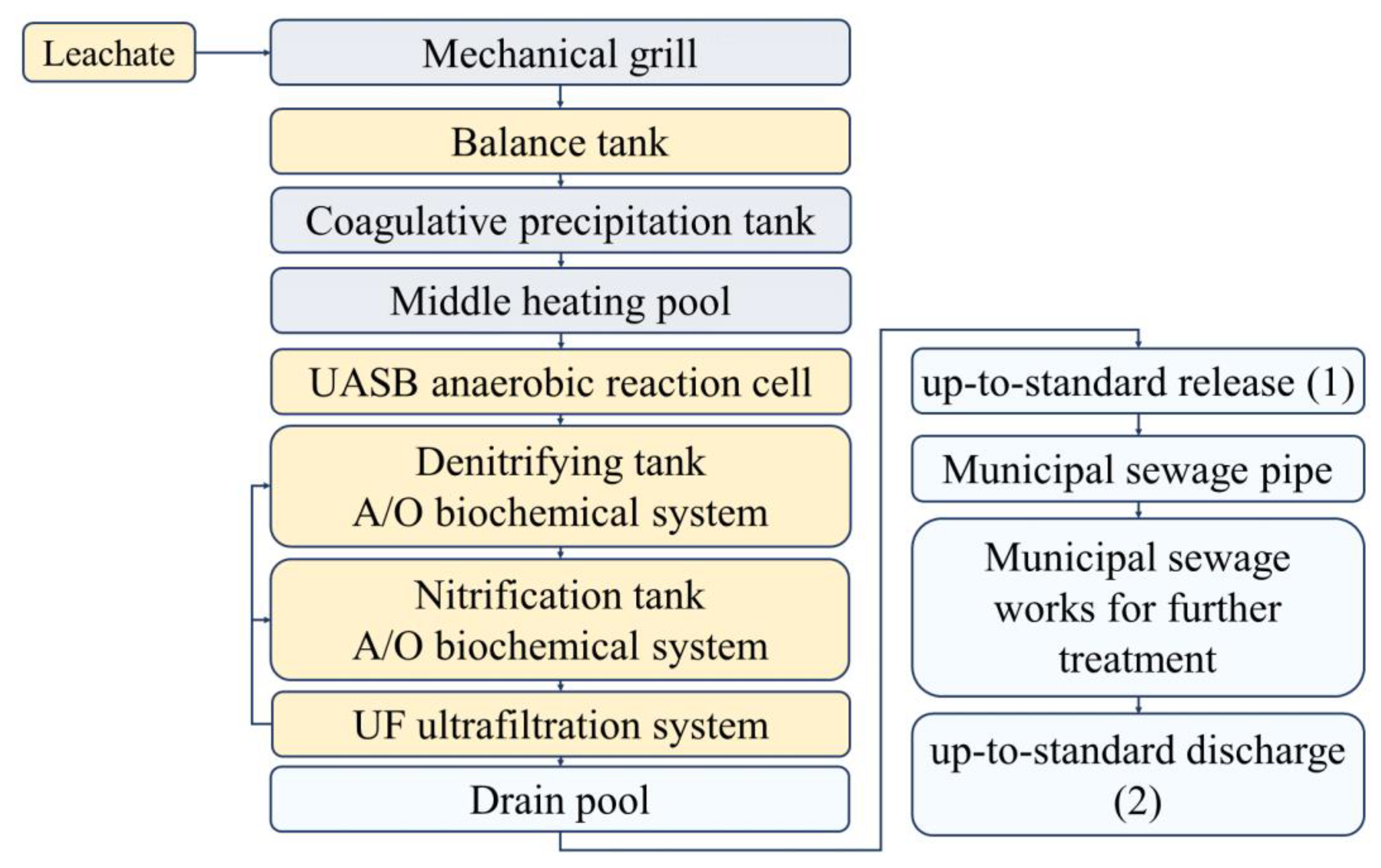
2.1. Sample Collection

The incineration leachate samples collected were from Wenling Green New Energy Co., Ltd. (Wenling, China), which was invested in by Zheneng Jinjiang Environment Holding Co., Ltd. (Hangzhou, China), who is a forerunner and leading waste-to-energy operator in China’s waste-to-energy (WTE) industry. The Wenling incineration power generation plant is located in the northern part of the Eastern New District of Wenling City, next to the East China Sea, with a total area of 7.3 × 10⁵ sqm. The leachate treatment scale of the incineration plant is 1600 tons/day in two phases, and for now, the treatment scale of the first phase is 800 tons/day (600 tons/day of domestic waste and 200 tons/day of dry sludge). The leachate treatment process of the incineration power plants is shown in Figure 1.

Leachate samples from six water outlets were collected on the 15 July 2022. In Figure 2, the samples from six water outlets were named leachate raw water (LRW), leachate effluent (LE), internal circulation reactor effluent, aerobic effluent (AeroE), anaerobic effluent (ANE), and MBR effluent (MBRE). The samples were preserved in a refrigerator at a temperature lower than 4 °C and were forwarded to the laboratory.

2.2. Chemical Parameters Detection for Incinerator Leachate

In general, incinerator leachate is tested by conventional parameters, including pH, chemical oxygen demand (COD), biochemical oxygen demand after 5 days (BOD₅), ammonia (NH4+-N), and total phosphorus (TP). The values of those conventional parameters exhibit considerable differences due to variations in composition and moisture content, as well as seasonal factors and incinerator location. The value of pH was tested by the electrode method [15]. For COD detection, the dichromate method is not suitable for the water samples in which the chloride ion concentration is higher than 1000 mg/L. The chlorine emendation method was applied to detect the contents of COD in the incinerator leachate samples [16]. The concentration of ammonia nitrogen was measured according to Nessler’s reagent spectrophotometry [17]. The alkaline potassium persulfate digestion UV spectrophotometric method [18] was used to detect total nitrogen content. The ammonium molybdate spectrophotometric method [19] was applied to detect the content of TP.

2.3. E-nose Detection

The EN mainly consists of two parts: the sensor array, which is applied to sense the information in the sample’s headspace, and the software part, which handles the information received from the sensors. According to the sensing materials, metal-oxide-semiconductor (MOS), quartz crystal microbalance, and surface acoustic wave sensors are most applied in the EN system [20]. MOS gas sensors are most sensitive to hydrogen and unsaturated hydrocarbons or solvent vapors containing hydrogen atoms [21]. The headspace gas from incinerator leachate contents is mainly composed of volatile organic compounds (VOCs), including hydrogen sulphide, methyl mercaptan, acetylene, propylene, and ethylene, and also varies according to source, season, the incinerator site, and so on [22].

A commercial PEN2 electronic nose (Airsense Analytics, GmBH, Schwerin, Germany) was applied to detect the headspace gas from incinerator leachate samples at different processing procedures. For PEN2, MOS sensors are the core part, and the details of MOS sensors are presented in

Table 1. Sensors used and their main applications in the EN.

No.	Sensor Name	General Description	Reference
S1	W1C	Aromatic compounds	Toluene, 0.1 g/kg
S2	W5S	Very sensitive with negative signal, broad range sensitivity, react on nitrogen oxides	NO2, 1 × 10−3 g/kg
S3	W3C	Very sensitive with aromatic compounds	Benzene, 1 × 10−2 g/kg
S4	W6S	Mainly hydrogen, selectively, (breath gases)	H2, 0.1 g/kg
S5	W5C	Alkanes, aromatic compounds, less polar compounds	Propane, 1 × 10−3 g/kg
S6	W1S	Sensitive to methane (environment). Broad range, similar to S8;	CH4, 0.1 g/kg
S7	W1W	Reacts on sulfur compounds, or sensitive to many terpenes and sulfur organic compounds;	H2S, 1 × 10−4 g/kg
S8	W2S	Detects alcohol’s, partially aromatic compounds, broad range	CO, 0.1 g/kg
S9	W2W	Aromatics compounds, sulfur organic compounds	H2S, 1 × 10−3 g/kg
S10	W3S	Reacts on high concentrations > 0.1 g/kg, sometime very selective (methane)	CH4, 0.1 g/kg

. The MOS sensors convert the information about gas types and concentrations into an electrochemical signal. The EN signal was expressed as G/G0, where G and G0 represent the resistance of a sensor in sample headspace gas and clean air. As the sensors are cross-sensitive to a class of gas compounds, EN does not give the specific information of one material but offers the headspace gas complementary information.

During the EN detection, incinerator leachate liquid with a 5 mL volume was placed into a 500 mL beaker. The beaker was sealed by plastic wrap and was kept still for 30 min to balance the headspace gas generated from the incinerator leachate. Two holes were made, one for EN detection and the other for a steady stream of gas while EN detecting. The EN detection time was set to 80 s, and then the gas path and sensor chamber were cleaned with clean air. The gas flow rate was 200 mL/min, and one signal per second was collected. Landfill leachate was collected from six water outlets with 24 samples; thus, 144 samples (24 samples × 6 procedures) were prepared. All the detection was accomplished on the sample collection day.

2.4. Data Reduction Based on Manifold Learning

2.4.1. Principal Component Analysis

As a multivariate technique, Principal Component Analysis (PCA) was applied to analyze a data set consisting of several inter-correlated quantitative dependent variables [23]. By calculating eigenvalue and eigenvector from the covariance matrix of the original data set, the new orthogonal variables will be derived and usually called principal components (PC). The cumulative contribution rate of PCs should reach more than 85% of the total variance, then the PCA will be considered to have extracted the main information of the original data.

2.4.2. Isometric Feature Mapping

As a nonlinear dimensionality reduction technique, Isometric Feature Mapping (ISOMAP) maintains the essential geometric structure of nonlinear data [24]. ISOMAP is multidimensional scaling combined with geodesic distance for reducing the dimensionality of data sampled from a smooth manifold. ISOMAP tries to solve the shortest path to obtain the geodesic distance that preserves the characteristics of high-dimensional data structures as much as possible. Multidimensional scaling is used to calculate the coordinates of each data point in the low-dimensional space, and the original data is embedded in the high-dimensional set.

2.4.3. Uniform Manifold Approximation and Projection

As a nonlinear dimensionality reduction technique, uniform manifold approximation and projection (UMAP) was developed for the analysis of any type of high-dimensional data [25]. From a theoretical framework based in Riemannian geometry and algebraic topology, UMAP learns the data representation between points in high-dimensional space and maps to low dimensions by calculating the joint probability density between high-dimensional sample points. Spectral clustering analysis is used to initialize the low-dimensional data and then project it into the low-dimensional space. Adjustable parameters are used in joint probability density to control the change of conditional probability and ensure the symmetry of the data. Low-dimensional data also provides two parameters to adjust the aggregation of mapped data so that low-dimensional data can better fit high-dimensional spatial data.

2.5. Classification and Prediction

2.5.1. Classification and Regression Tree

Classification and Regression Tree (CART) selects features based on the minimization of the Gini coefficient to generate a binary tree. By pre-pruning through empirical judgment, the useless attributes can be removed. After the construction is completed, the algorithm can resist overfitting and has better generalization ability by cutting off a part of the information with less proportion.

In addition, the shortcomings that CART cannot handle large amounts of data, underfitting, and overfitting, can be overcome by integrating multiple CART classifiers into a single ensemble model with the ideas of bagging and boosting. The study selects a boosting algorithm with relatively stable generalization performance. Boosting is a kind of optimization algorithm based on the greedy strategy of selecting the fixed loss function (optimization function and objective function) based on a greedy strategy for the optimization of the loss function, committed to obtaining the minimum loss optimization function, such as eXtreme Gradient Boosting (XGBT) and Light Gradient Boosting Machine (lightGBM).

2.5.2. eXtreme Gradient Boosting

eXtreme Gradient Boosting (XGBT) uses the first and second partial derivatives, and the second derivatives help the gradient descend faster and more accurately. Using Taylor expansion to obtain the function as the second derivative form of the independent variable, the leaf splitting optimization calculation can be carried out only by relying on the value of the input data without selecting the specific form of the loss function, essentially separating the selection of the loss function from the optimization of the model algorithm/parameter selection [26]. The algorithm goes:

1. Initialize model with a constant value:

$${\widehat{f}}_0\left(x\right)=\mathrm{argmin}{\displaystyle \sum }_i^{n}L\left(y_i,\theta \right)$$

For m = 1 to M:

a. Compute so-called pseudo-residuals:

$${\widehat{g}}_m\left(x\right)=-{\left[\frac{\partial L\left(y_i,f(x_i\right))}{\partial f\left(x_i\right)}\right]}_{f\left(x\right)={\widehat{f}}_{m-1}\left(x\right)}$$

$${\widehat{h}}_m\left(x\right)=-{\left[\frac{{\partial }^{2}L\left(y_i,f(x_i\right))}{\partial f{\left(x_i\right)}^2}\right]}_{f\left(x\right)={\widehat{f}}_{m-1}\left(x\right)}$$

b. Fit a base learner using the training set ${\displaystyle \{}{x}_i,{\frac{{\widehat{g}}_m\left(x_i\right)}{{\widehat{h}}_m\left(x_i\right)}{\displaystyle \}}}_{i=1}^n$ by solving the optimization problem below:

$${\widehat{\phi }}_m=argmin{\displaystyle \sum }_i^N\frac{1}{2}{\widehat{h}}_m\left(x_i\right){\left[-\frac{{\widehat{g}}_m\left(x_i\right)}{{\widehat{h}}_m\left(x_i\right)}-\phi \left(x_i\right)\right]}^2$$

$${\widehat{f}}_m\left(x\right)=\alpha {\widehat{\phi }}_m\left(x\right)$$

c. Update the model:

$${\widehat{f}}_m\left(x\right)={\widehat{f}}_{m-1}\left(x\right)+{\widehat{f}}_m\left(x\right)$$

2. output $F_M\left(x\right)$.

2.5.3. Light Gradient Boosting Machine

Light Gradient Boosting Machine (LightGBM) grows trees leaf-wise instead of level-wise, yielding the largest loss decrease. LightGBM implements a highly optimized histogram-based decision tree learning algorithm, which greatly improves efficiency and memory consumption [27]. The algorithm goes:

(1)

The sample points are sorted in descending order according to the absolute value of their gradient;

(2)

Select the first samples of the sorted results to generate a subset of large gradient sample points;

(3)

For 100% samples of the remaining sample set (1 − a), randomly select b (1 − a) × 100% sample points to generate a set of small gradient sample points;

(4)

Merge the large gradient samples with the sampled small gradient samples;

(5)

Multiply the small gradient samples by a weight coefficient;

(6)

Learn a new weak learner (CART) using the above-sampled samples;

(7)

Continuously repeat steps (1)~(6) until the specified number of iterations or convergence is reached.

2.6. The Evaluation of Data Processing

To evaluate the accuracy and precision of the established models, 100 samples were set as the training data, and the rest, 44 samples, were set as the testing data.

The receiver operative curve (ROC) was deployed as a performance indicator for the classification models. True positive and negative rates are the most commonly used to evaluate the performance of classification tests. The higher the probability value of these two indicators, represents the better the judgment effect in the model [28].

The coefficient R² and RMSE were selected as the evaluation parameters for prediction models. The higher the R² was and the lower the RMSE was, the more accurate the prediction ability of the model would be.

3. Results and Discussion

3.1. The Chemical Parameter Changes of Leachate

The composition of leachate is highly variable and heterogeneous. In general, incinerator leachate is tested using conventional parameters, including pH, COD, BOD₅, ammonia, and TP. The changes in the chemical parameters for leachate samples are shown in

Table 2. Average values of leachate chemical parameters.

	pH	COD (mg/L)	BOD5 (mg/L)	Ammonia (mg/L)	TN (mg/L)	TP (mg/L)
LRW	8b	4.23 × 103 f	1.10 × 103 c	1.92 × 103 d	2.18 × 103 c	15.4 b
RPE	8b	6.14 × 103 e	1.50 × 103 d	1.70 × 103 c	2.14 × 103 c	24.3 c
ICRE	8.1b	2.90 × 103 d	0.70 × 103 b	1.54 × 103 c	1.76 × 103 b	24.1 c
AnE	8.3b	2.00 × 103 c	0.52 × 103 b	0.71 × 103 b	1.32 × 103 a	15.2 b
AeroE	7.8b	1.5 × 103 b	0.10 × 103 a	0.12 × 103 a	1.20 × 103 a	10.3 a
MBRE	6a	0.33 × 103 a	0.09 × 103 a	0.04 × 103 a	1.13 × 103 a	4.61 a

The values are the average of the total score of the ten experts with respect to three replications of leachate samples. Mean in the same row followed by different inline letters (a, b, c, d, e, f) is statistically different as confirmed by Tukey’s HSD test (p < 0.05).

. There were statistically significant differences (Turkey HSD, p < 0.05) in the contents of COD, BOD₅, ammonia, TN, and TP. It was noteworthy that the values of COD decreased significantly at each process procedure. The changes were also noticeable for BOD, ammonia, TN, and TP. Different from the other five chemical parameters, the value of pH changes a lot at the last processing procedure. All the chemical parameters were all up to standard, when the processed leachate was discharged to the municipal pipe network.

3.2. The Result of EN Detection

The EN was used to analyze the headspace gas of the leachate samples at different process periods. A typical response of the EN sensors array during exposure to sample gas, which was randomly selected from the 144 samples, is depicted in Figure 3a. The procedure of extracting the sample gas from the beaker to the sensing chamber took 5 seconds, and then the sensors could react with the gas. The sensor signals changed significantly from 5 to 35 s, and then the signals achieved a dynamic equilibrium. The various signal values (maximum or minimum), the shifts, the response areas, and so on indicated that the sensors offered unique and abundant characteristics about the headspace gas of the leachate samples. To simplify data processing, sensor signals at 80th second were selected as the input data of the analysis models. To fully understand the sensor signals, the average values of 10 sensors were calculated and shown in Figure 3b. The overall signals (at the 80th second) varied a lot in the first three process periods (LRW, LE, and ICRE), and for ANE, AeroE, and MBRE samples, the signals changed not so remarkably. To further analyze the behaviors of those sensors, a radar fingerprint chart of EN signals is shown in Figure 3c: S2, the most sensitive sensor, showed the biggest variance, and S10 stayed almost still, and S10 stayed almost still. The impacts of leachate headspace gas on the responses of S8, S6, S9, and S5 were to different degrees, and those on S7 and S4 were not so obvious.

3.3. Data Reduction Based on Manifold Learning

Data reduction helps transfer an abundant and disordered original data set into a simplified and ordered form. PCA is a popular technology in dimensionality reduction and is flexible, fast, and easily interpretable. PCA does not perform well when there are nonlinear relationships within the data. For high-dimensional data, it is difficult to affirm whether the EN data is linear or not linear. ISOMAP and UMAP, as two kinds of manifold learning, were applied and compared with PCA.

The best description of differences in the original data can be found by calculating the eigen-decomposition of positive semi-definite matrices and the singular value decomposition of rectangular matrices. The PCs are ordered by ranking according to their contribution (eigenvalue). In Figure 4a, the contributions of PCs are displayed, and the first three PCs have extracted the most information from the original EN data at the 80th second (more than 85%). The sample distributions of 144 samples based on the first three PCs (PC1, PC2, and PC3) are shown in Figure 4b. LPW, LE, and ICRE can be easily classified, but ANE, AeroE, and MBRE are overlapped in a three-dimensional space. The result is similar to those shown in Figure 3b in some ways.

ISOMAP constructs the geodesic distance graph from the original EN data, and uses eigenvalue decomposition of MDS on the geodesic distance matrix to achieve low-dimensional embeddings. The ICs are ordered and displayed by ranking the contribution in Figure 5a. The first three ICs also extracted the most information of the original EN data at 80th second (more than 85%), which are very similar to that in Figure 4a. Because PCA and ISOMAP used eigen-decomposition and eigenvalue in this study, but there were minuscule differences in the data. The sample distributions based on the first three ICs are shown in Figure 5b. Similar as in Figure 4b, LPW, LE, and ICRE can be easily classified, but ANE, AeroE, MBRE overlapped.

UMAP preserves the local and global data structures and offers short run times based on Riemannian geometry and algebraic topology. Calculating the distance between embedding spaces is an approximate measure to determine how sensitive the canonical embedding space’s topology is, which is the feature importance. Figure 6a provides a careful look at the feature importance of 10 UCs, which is quite different from Figure 4a and Figure 5a. The first three UCs obviously did not extract more than 85% of the information from the original EN data, but not meaning that UMAP would do badly for later classification and prediction. In Figure 6b, most of the samples seem to be clustered narrowly. LPW, LE, and ICRE are classified clearly and can be easily distinguished in a three-dimensional space. ANE and AeroE are overlapped, along with two MERE samples. In general, in three-dimensional space, UMAP outperformed the PCA and ISOMAP in Figure 4b and Figure 5b.

3.4. Classification Based on EN Signals

3.4.1. Classification Result Based on LightGBM

ROC graphs are used to organize classifiers and visualize the results. As can be seen from the ROC curve of the lightGBM in Figure 7, the classification accuracy results of the original, PCA, ISOMAPa, and UMAP data are very different in the training set, respectively. In the view of the lightGBM models, the PCA better retains the majority of the information of the original data set according to the ROC curve, and the overall AUC area reaches 100%. From the ROC results, the performance of UMAP was better than that of ISOMAP, and only one category 6 classification showed partial errors. In the ISOMAP-lightGBM model, samples from classes 4 and 6 were misclassified.

To explore further the models based on different data sets, testing data sets were applied to verify the classification result. Moreover, to reduce the volatility attributable, each model was run 20 times, and the average results are displayed in

Table 3. The classification results in the training set and testing set based on lightGBM.

Model	Accurate Rate in the Training Set (%)	Accurate Rate in the Testing Set (%)
Original-lightGBM	100	96.25
PCA-lightGBM	100	94.44
ISOMAP-lightGBM	100	96.81
UMAP-lightGBM	99.95	97.36

. The best classification performance is the UMAP-XGBT model, with a 99.95% accuracy rate in the training set and a 97.36% accuracy rate in the testing set, indicating that UMAP-XGBT has the most stable robustness. For PCA-lightGBM, the classification results were worse than those of the original-lightGBM model in the testing set. ISOMAP-lightGBM has a 100% average accuracy rate in the training set and a 96.81 average accuracy rate in the testing set.

3.4.2. Classification Result Based on XGBT

According to the ROC results in Figure 8, the best performance of classification models is PCA-XGBT, with only two error classification cases. In the UMAP-XGBT model, samples of LE and AeroE were misclassified, but the overall performance was better than that of the original-XGBT. The ISOMAP-XGBT model, with the worst classification performance, has categories LE and AeroE misclassified. According to the training set, ISOMAP-XGBT has the worst performance.

For XGBT models, the data training took 20 times to decrease the instability, and the result is shown in

Table 4. The classification results in the training set and testing set based on XGBT.

Model	Accurate Rate in the Training Set (%)	Accurate Rate in the Testing Set (%)
Original-XGBT	100	94.72
PCA-XGBT	100	93.61
ISOMAP-XGBT	100	95.28
UMAP-XGBT	99.95	95.83

. The accuracy rates of XGBT models were lower than those of the lightGBM-based models. From Table 4, it can be concluded that the UMAP-XGBT model had the best classification performance, with a 99.95% accuracy rate in the training set and a 95.83% accuracy rate in the testing set.

From Table 3 and Table 4, models of original-XGBT, PCA-XGBT, and ISOMAP-XGBT always had a satisfying performance with a 100% accuracy rate in the training set in the 20 times it was run, while they fell short in the testing set. This might be because the models were overfit in the modeling, so the results in the testing set were not very good.

3.5. Chemical Parameter Prediction Based on EN Signals

3.5.1. Prediction Results Based on LightGBM

As an ensemble learning program, lightGBM aims to build a comprehensive model by parallelizing and serializing weak learners (CART). For lightGBM models, a histogram-based algorithm and tree leaf-wise growth strategy with a maximum depth limit are adopted to increase the training speed. For lightGBM, the max-features was set 4, and the tree leaf-wise was set 3 to simplify the lightGBM model in preliminary work. Then, the number of decision trees was the most important parameter in the later modeling. The number of CARTs was optimized, and the optimization procedure is carried out in Figure 9 (taking COD prediction as an example) according to the R²s and EMSEs in the training set and testing set. The lightGBM was 20 times for each number of CARTs to minimize the contingency. As shown in Figure 9, the results in the training set have stable precision with the increasing decision tree numbers. While the result precision in the testing set was not stable regardless of which data set was applied. All in all, the lightGBM model with the UMAP data set had a slight advantage (not so obvious) when compared to the other three data sets. When the number of CARTs was 25, the lightGBM model showed a satisfactory result. The best number of CARTs for the lightGBM model was decided.

EN signals offered the entirety of the information on leachate headspace gas, which mainly consisted of volatile organic compounds (VOCs), including hydrogen sulphide, methyl mercaptan, acetylene, and so on. The materials in the headspace gas were most closely correlated to the value of COD. The EN combined with the data mining method could predict the contents of COD in leachate samples.

Table 5. Comparison of the LightGBM prediction models based on different manifold learning methods.

Data Set		R2 (Training)	RMSE (Training)	R2 (Testing)	RMSE (Testing)	Data Set		R2 (Training)	RMSE (Training)	R2 (Testing)	RMSE (Testing)
Original data	pH	0.9721	0.2278	0.7217	0.6870	PCA	pH	0.9258	0.3716	0.8690	0.4521
	COD	0.9987	120.72	0.9779	492.01		COD	0.9968	189.74	0.9916	302.91
	BOD	0.9991	27.82	0.9843	110.01		BOD	0.9968	50.89	0.9893	94.20
	AN	0.9991	40.66	0.9753	208.42		AN	0.9974	68.20	0.9957	87.06
	TN	0.9953	52.35	0.9785	110.42		TN	0.9857	90.85	0.9694	132.52
	TP	0.9978	0.5781	0.9347	3.11		TP	0.9952	0.8652	0.9739	2.02
ISOMAP	pH	0.9211	0.3834	0.8793	0.4286	UMAP	pH	0.9806	0.1339	0.9803	0.1721
	COD	0.9968	189.29	0.9963	202.01		COD	0.9989	113.43	0.9881	356.88
	BOD	0.9967	51.98	0.9921	80.49		BOD	0.9991	27.82	0.9947	66.30
	AN	0.9973	68.55	0.9959	85.75		AN	0.9991	40.52	0.9938	105.89
	TN	0.9837	96.96	0.9701	130.60		TN	0.9952	52.45	0.9933	62.07
	TP	0.9953	0.8512	0.9844	1.51		TP	0.9982	0.5229	0.9895	0.5742

summarizes the prediction results based on different data reductions for five chemical parameters (pH, COD, BOD₅, AN, TN, and TP). According to the R²s and EMSEs in the training set and testing set, the PCA process had no effect on the lightGBM models compared to models based on original data. LightGBM models based on ISOMAP and UMAP showed satisfactory outcomes. The prediction of five chemical parameters based on the UMAP-lightGBM model showed the best performance with an R² higher than 0.98 in the training set and testing set (RMSEs are not comparable when it comes to different parameters and units).

3.5.2. Prediction Results Based on XGBT

As with lightGBM, the parameters of the XGBT models, including the number of trees, maximal depth, and minimum rows, were optimized. Finally, the max-features was set 4, max-depth was set 2, and min-split was set 2 to simplify the XGBT model. The number of decision trees (CART) was the most important parameter in the later modeling. The optimization procedure is carried out in Figure 10 (taking COD prediction as an example) according to the R²s and EMSEs in the training set and testing set, 20 times for each modeling step to minimize the contingency. As shown in Figure 10, the overall prediction performance of XGBT models was much better than lightGBM in Figure 10. XGBT models have very strong robustness and stability, particularly for the ISOMAP-XGBT models in Figure 10c. When the number of decision trees was 25, the XGBT models had a relatively satisfactory result, meanwhile the model was not so big, the same as the lightGBM models.

Table 6. Comparison of the XGBT prediction models based on different manifold learning methods.

Data Set		R2 (Training)	RMSE (Training)	R2 (Testing)	RMSE (Testing)	Data Set		R2 (Training)	RMSE (Training)	R2 (Testing)	RMSE (Testing)
Original data	pH	0.9721	0.2278	0.7217	0.6870	PCA	pH	0.9258	0.3716	0.8690	0.4521
	COD	0.9987	120.72	0.9779	492.01		COD	0.9968	189.74	0.9916	302.91
	BOD	0.9991	27.82	0.9843	110.01		BOD	0.9968	50.89	0.9893	94.20
	AN	0.9991	40.66	0.9753	208.42		AN	0.9974	68.20	0.9957	87.06
	TN	0.9953	52.35	0.9785	110.42		TN	0.9857	90.85	0.9694	132.52
	TP	0.9978	0.5781	0.9347	3.11		TP	0.9952	0.8652	0.9739	2.02
ISOMAP	pH	0.9861	0.1834	0.9803	0.1986	UMAP	pH	0.9806	0.1939	0.9833	0.1721
	COD	0.9968	189.29	0.9963	202.01		COD	0.9989	113.43	0.9901	156.88
	BOD	0.9967	51.98	0.9921	80.49		BOD	0.9991	27.82	0.9947	66.30
	AN	0.9973	68.55	0.9959	85.75		AN	0.9991	40.52	0.9938	105.89
	TN	0.9837	96.96	0.9701	130.60		TN	0.9952	52.45	0.9933	62.07
	TP	0.9953	0.8512	0.9844	1.51		TP	0.9982	0.5229	0.9975	0.5574

summarizes the prediction results based on different data reductions for five chemical parameters. All in all, prediction results based on XGBT have achieved better results compared to lightGBM models. Different from PCA-lightGBM models, PCA-XGBT models have a slight edge over the (original data)-XGBT models in the testing set. The prediction of five chemical parameters based on the UMAP-XGBT model showed the best performance with an R² higher than 0.99 in the training set and testing set.

For prediction models, the overall performances of XGBT models are better than those of lightGBM, and the data set based on UMAP reduction has a slight advantage both in the training set and the testing set when compared to other three data sets.

4. Conclusions

MSW incineration is regarded as an ideal method for MSW disposal, with many advantages. This study applied an EN detection method for monitoring MSW incinerator leachate combined with manifold learning and ensemble methods. Some conclusions can be drawn:

(1)

COD, BOD5, ammonia, TN, and TP of leachate were significantly changed during the processing procedure, especially for COD;

(2)

EN sensors offered unique and abundant characteristics of leachate samples in the headspace gas. The signals at the 80th second varied a lot in the first three process periods (LRW, LE, and ICRE), for ANE, AeroE, and MBRE samples, the signals changed not so remarkably;

(3)

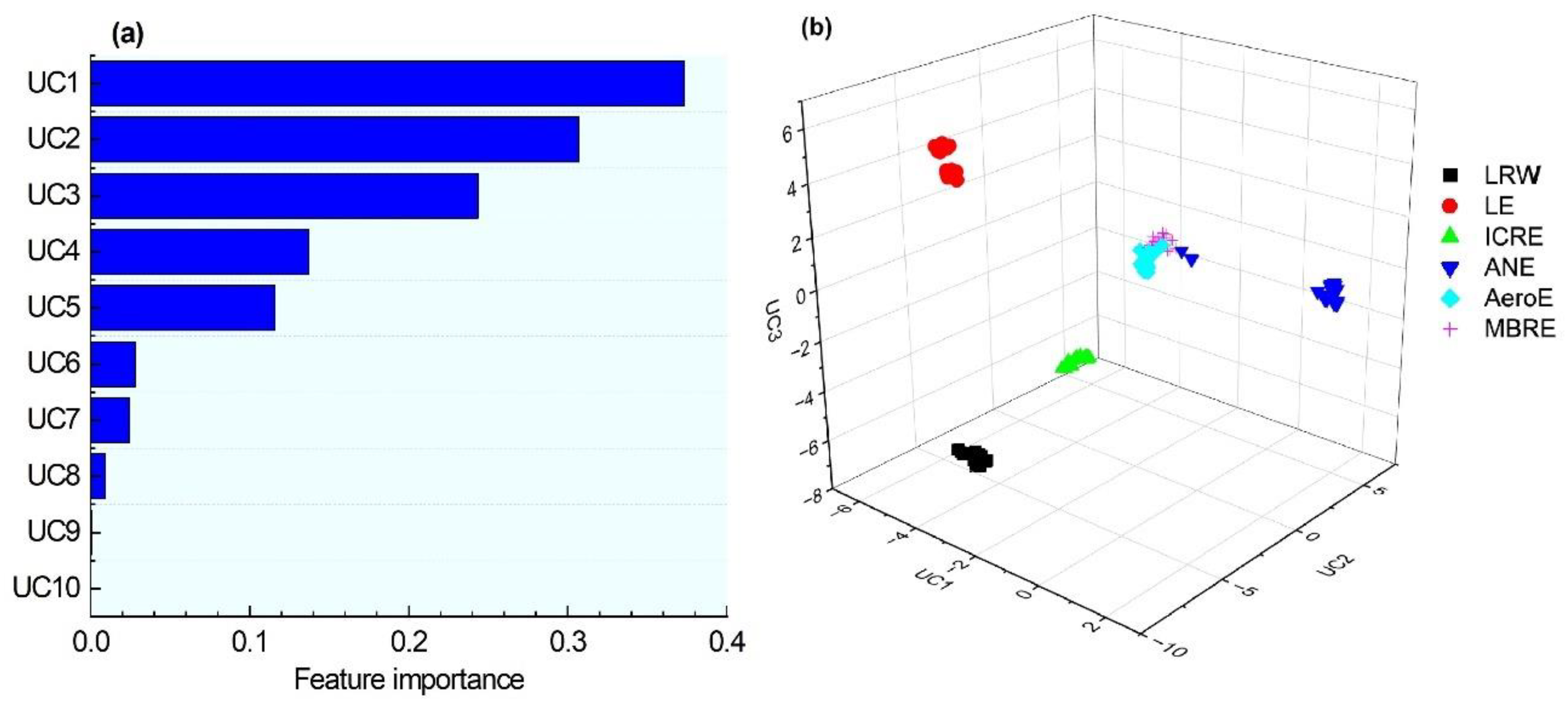
Manifold learnings (PCA, ISOMAP, and UMAP) were applied to extract the information hidden in the headspace gas of leachate detected by EN. The first three PCs and ICs have extracted the most information from the original data (>85%), and samples of LPW, LE, and ICRE could be easily classified according to the three-dimensional space, while others were not so satisfied. UMAP outperformed the performance of PCA and ISOMAP;

(4)

Ensemble methods (LightGBM and XGBT) were applied to mine the relationship between EN signals of leachate headspace gas and chemical parameter changes combined with PCA, ISOMAP, and UMAP. The UMAP-XGBT model had the best classification performance, with a 99.95% accuracy rate in the training set, and a 95.83% accuracy rate in the testing set. The UMAP-XGBT model showed the best prediction ability for the leachate chemical parameters R² higher than 0.99 in the training and testing sets.

Up until now, there have been few in-depth studies that have been conducted to fetch information from the headspace gas of leachate samples. This is the first study with an EN application for leachate monitoring based on manifold learning and ensemble methods, offering an easier and quicker monitoring method than traditional instrumental measurements. Future work will focus on the potential relationship between microorganisms and headspace gas in the leachate based on EN technology to fully understand the MSW incineration leachate chemical parameter changes, which is quite important for leachate disposal.

References

1. Kaza:, S.; Yao, L.C.; Bhada-Tata, P.; Van Woerden, F. What a Waste 2.0: A Global Snapshot of Solid Waste Management to 2050. Urban Development; World Bank: Washington, DC, USA, 2018; Available online: https://openknowledge.worldbank.org/handle/10986/30317 (accessed on 1 November 2022).
2. Lippi, M.; Ley, M.B.R.G.; Mendez, G.P.; Cardoso Junior, R.A.F. State of Art of Landfill Leachate Treatment: Literature Review and Critical Evaluation. Ciência Nat. 2018, 40, e78. [Google Scholar] [CrossRef] [Green Version]
3. Cudjoe, D.; Han, M.S. Economic feasibility and environmental impact analysis of landfill gas to energy technology in African urban areas. J. Clean. Prod. 2021, 284, 125437. [Google Scholar] [CrossRef]
4. Shah, A.V.; Srivastava, V.K.; Mohanty, S.S.; Varjani, S. Municipal solid waste as a sustainable resource for energy production: State-of-the-art review. J. Environ. Chem. Eng. 2021, 9, 105717. [Google Scholar] [CrossRef]
5. Ren, X.; Liu, D.; Chen, W.; Jiang, G.; Wu, Z.; Song, K. Investigation of the characteristics of concentrated leachate from six municipal solid waste incineration power plants in China. RSC Adv. 2018, 8, 13159–13166. [Google Scholar] [CrossRef] [Green Version]
6. Chen, W.; He, C.; Zhuo, X.; Wang, F.; Li, Q. Comprehensive evaluation of dissolved organic matter molecular transformation in municipal solid waste incineration leachate. Chem. Eng. J. 2020, 400, 126003. [Google Scholar] [CrossRef]
7. Jiang, F.; Qiu, B.; Sun, D. Degradation of refractory organics from biologically treated incineration leachate by VUV/O3. Chem. Eng. J. 2019, 370, 346–353. [Google Scholar] [CrossRef]
8. Hu, W.; Wan, L.; Jian, Y.; Ren, C.; Jin, K.; Su, X.; Bai, X.; Haick, H.; Yao, M.; Wu, W. Electronic Noses: From Advanced Materials to Sensors Aided with Data Processing. Adv. Mater. Technol. 2019, 4, 1800488. [Google Scholar] [CrossRef] [Green Version]
9. Eusebio, L.; Derudi, M.; Capelli, L.; Nano, G.; Sironi, S. Assessment of the Indoor Odour Impact in a Naturally Ventilated Room. Sensors 2017, 17, 778. [Google Scholar] [CrossRef] [Green Version]
10. Bieganowski, A.; Józefaciuk, G.; Bandura, L.; Guz, Ł.; Łagód, G.; Franus, W. Evaluation of Hydrocarbon Soil Pollution Using E-Nose. Sensors 2018, 18, 2463. [Google Scholar] [CrossRef] [Green Version]
11. Tonacci, A.; Sansone, F.; Conte, R.; Domenici, C. Use of Electronic Noses in Seawater Quality Monitoring: A Systematic Review. Biosensors 2018, 8, 115. [Google Scholar] [CrossRef]
12. Jońca, J.; Pawnuk, M.; Arsen, A.; Sówka, I. Electronic Noses and Their Applications for Sensory and Analytical Measurements in the Waste Management Plants—A Review. Sensors 2022, 22, 1510. [Google Scholar] [CrossRef] [PubMed]
13. Tasaki, H.; Lenz, R.; Chao, J. Dimension Estimation and Topological Manifold Learning. In Proceedings of the 2019 International Joint Conference on Neural Networks (IJCNN), Budapest, Hungary, 14–19 July 2019; pp. 1–7. [Google Scholar]
14. Zounemat-Kermani, M.; Stephan, D.; Barjenbruch, M.; Hinkelmann, R. Ensemble data mining modeling in corrosion of concrete sewer: A comparative study of network-based (MLPNN & RBFNN) and tree-based (RF, CHAID, & CART) models. Adv. Eng. Inform. 2020, 43, 101030. [Google Scholar]
15. HJ 1147-2020; Ministry of Ecology and Environment of the People's Republic of China. Water Qulity—Determination of pH—Electrode Method. Ministry of Ecology and Environment of the People's Republic of China. Available online: https://max.book118.com/html/2020/1129/8117023002003022.shtm (accessed on 1 November 2022).
16. HJ/T 70-2001; High-Chlorine Wastewater—Determination of Chemical Oxygen Demand—Chlorine Emendation Method. Ministry of Ecology and Environment of the People's Republic of China. Available online: https://www.doc88.com/p-9982565679330.html?r=1 (accessed on 1 November 2022).
17. HJ 535-2009; Water Quality―Determination of Ammonia Nitrogen―Nessler’s Reagent Spectrophotometry. Ministry of Ecology and Environment of the People's Republic of China. Available online: http://www.doc88.com/p-6836770291709.html (accessed on 1 November 2022).
18. HJ 636-2012; Water Quality—Determination of Total Nitrogen—Alkaline Potassium Persulfate Digestion UV Spectrophotometric Method. Ministry of Ecology and Environment of the People's Republic of China. Available online: http://www.doc88.com/p-7187319550717.html (accessed on 1 November 2022).
19. GB/T 11893-1989; Water Quality—Determination of Total Phosphorus—Ammonium Molybdate Spectrophotometric Method. Ministry of Ecology and Environment of the People's Republic of China. Available online: https://www.doc88.com/p-6764771874050.html?r=1 (accessed on 1 November 2022).
20. Wilson, A.D. Review of Electronic-nose Technologies and Algorithms to Detect Hazardous Chemicals in the Environment. Procedia Technol. 2012, 1, 453–463. [Google Scholar] [CrossRef] [Green Version]
21. Dey, A. Semiconductor metal oxide gas sensors: A review. Mater. Sci. Eng. B 2018, 229, 206–217. [Google Scholar] [CrossRef]
22. Nair, A.T.; Senthilnathan, J.; ShivaNagendra, S.M. Emerging perspectives on VOC emissions from landfill sites: Impact on tropospheric chemistry and local air quality. Process Saf. Environ. Prot. 2019, 121, 143–154. [Google Scholar] [CrossRef]
23. Abdi, H.; Williams, L.J. Principal component analysis. Wiley Interdiscip. Rev. Comput. Stat. 2010, 2, 433–459. [Google Scholar] [CrossRef]
24. Gao, S.; Zhang, S.; Zhang, Y.; Gao, Y. Operational reliability evaluation and prediction of rolling bearing based on isometric mapping and NoCuSa-LSSVM. Reliab. Eng. Syst. Saf. 2020, 201, 106968. [Google Scholar] [CrossRef]
25. Becht, E.; McInnes, L.; Healy, J.; Dutertre, C.-A.; Kwok, I.W.H.; Ng, L.G.; Ginhoux, F.; Newell, E.W. Dimensionality reduction for visualizing single-cell data using UMAP. Nat. Biotechnol. 2019, 37, 38–44. [Google Scholar] [CrossRef]
26. Kumari, P.; Toshniwal, D. Extreme gradient boosting and deep neural network based ensemble learning approach to forecast hourly solar irradiance. J. Clean. Prod. 2021, 279, 123285. [Google Scholar] [CrossRef]
27. Taha, A.A.; Malebary, S.J. An Intelligent Approach to Credit Card Fraud Detection Using an Optimized Light Gradient Boosting Machine. IEEE Access 2020, 8, 25579–25587. [Google Scholar] [CrossRef]
28. Chang, Y.-C.; Chang, K.-H.; Wu, G.-J. Application of eXtreme gradient boosting trees in the construction of credit risk assessment models for financial institutions. Appl. Soft Comput. 2018, 73, 914–920. [Google Scholar] [CrossRef]
Figure 1. Process flow diagram of incineration leachate treatment in the study.
Chemosensors 10 00506 g001
Figure 2. Leachate sample collection: (a) leachate raw water (LRW), (b) leachate effluent (LE), (c) internal circulation reactor effluent (ICRE), (d) aerobic effluent (AeroE), (e) Anaerobic effluent (ANE), and (f) MBR effluent (MBRE).
Chemosensors 10 00506 g002
Figure 3. A typical response of EN sensor array during exposure to sample gas: (a) a typical response of EN during leachate detection, (b) the average values of EN signals at the 80th second, and (c) a radar fingerprint chart of EN signals.
Chemosensors 10 00506 g003
Figure 4. EN data reduction based on PCA: (a) PCs ordered according the eigenvalues, (b) sample distributions based on the first three PCs.
Chemosensors 10 00506 g004
Figure 5. EN data reduction based on ISOMAP: (a) ICs ordered according the eigenvalues, (b) sample distributions based on the first three ICs.
Chemosensors 10 00506 g005
Figure 6. EN data reduction based on UMAP: (a) UCs ordered according the eigenvalues, (b) sample distributions based on the first three UCs.
Chemosensors 10 00506 g006
Figure 7. Overall receiver operating characteristics (ROC) curve of lightGBM showing the true positive and false-positive: (a) based on original data, (b) based on the PCA data, (c) based on the ISOMAP data, and (d) based on the UMAP data. Class S1 refers to LRW samples, class S2 refers to LE, class S3 refers to ICRE, class S4 refers to AeroE, class S5 refers to ANE, and class S6 refers to MBRE.
Chemosensors 10 00506 g007
Figure 8. Overall receiver operating characteristics (ROC) curve of XGBT showing the true positive and false-positive: (a) based on the original data, (b) based on the PCA data, (c) based on the ISOMAP data, and (d) based on the UMAP data. Class S1 refers to LRW samples, class S2 refers to LE, class S3 refers to ICRE, class S4 refers to AeroE, class S5 refers to ANE, and class S6 refers to MBRE.
Chemosensors 10 00506 g008
Figure 9. The performance of lightGBM according to the numbers of decision trees: (a) based on the original data set, (b) based on the PCA data set, (c) based on the ISOMAP data set, and (d) based on the UMAP data set.
Chemosensors 10 00506 g009
Figure 10. The performance of XGBT according to the numbers of decision trees: (a) based on the original data set, (b) based on the PCA data set, (c) based on the ISOMAP data set, (d) based on the UMAP data set.
Chemosensors 10 00506 g010