Article

Using Near-Infrared Spectroscopy and Stacked Regression for the Simultaneous Determination of Fresh Cattle and Poultry Manure Chemical Properties

by
Elizabeth Cobbinah
1,†,
Oliver Generalao
2,†,
Sathish Kumar Lageshetty
3,
Indra Adrianto
4,5,
Seema Singh
6 and
Gerard G. Dumancas
1,*
1
Department of Chemistry, Loyola Science Center, The University of Scranton, Scranton, PA 18510, USA
2
Center for Informatics, University of San Agustin, Gen. Luna St, Iloilo City 5000, Philippines
3
Research and Development Department, CHASM Advanced Materials, 2501 Technology Place, Norman, OK 73071, USA
4
Department of Public Health Sciences, Henry Ford Health, Detroit, MI 48202, USA
5
Department of Medicine, Michigan State University, East Lansing, MI 48824, USA
6
Sandia National Laboratories and Joint Bioenergy Institute, Livermore, CA 94550, USA
*
Author to whom correspondence should be addressed.
These authors contributed equally to this work.
Chemosensors 2022, 10(10), 410; https://doi.org/10.3390/chemosensors10100410
Submission received: 29 August 2022 / Revised: 30 September 2022 / Accepted: 8 October 2022 / Published: 11 October 2022
(This article belongs to the Collection Women Special Issue in Chemosensors and Analytical Chemistry)

Abstract

:
Excessive use of animal manure as fertilizers can lead to pollution through the introduction of nitrogen, phosphorus, and other mineral compounds to the environment. Wet chemical analytical methods are traditionally used to determine the precise chemical composition of manure to manage the application of animal waste to the soil. However, such methods require significant resources to carry out the processes. Affordable, rapid, and accurate methods of analyses of various chemical components present in animal manure, therefore, are valuable in managing soil and mitigating water pollution. In this study, a stacked regression ensemble approach using near-infrared spectroscopy was developed to simultaneously determine the amount of dry matter, total ammonium nitrogen, total nitrogen, phosphorus pentoxide, calcium oxide, magnesium oxide, and potassium oxide contents in both cattle and poultry manure collected from livestock production areas in France and Reunion Island. The performance of the stacked regression, an ensemble learning algorithm that is formed by collating the well-performing models for prediction was then compared with that of various other machine learning techniques, including support vector regression (linear, polynomial, and radial), least absolute shrinkage and selection operator, ridge regression, elastic net, partial least squares, random forests, recursive partitioning and regression trees, and boosted trees. Results show that stack regression performed optimally well in predicting the seven abovementioned chemical constituents in the testing set and may provide an alternative to the traditional partial least squares method for a more accurate and simultaneous method in determining the chemical properties of animal manure.

Graphical Abstract

1. Introduction

Animal manure has traditionally been used as a fertilizer to improve soil fertility and carbon sequestration, as well as support crop growth [1,2]. It contains essential nutrients including nitrogen (N), phosphorus (P), and potassium (K), which can improve soil quality and, thus, influence agronomic activities such as soil and crop management [3]. Most chemical nutrients existing in fertilizers are normally present in their oxide form; thus, P is present as phosphorus pentoxide (P2O5), K as potassium oxide (K2O), calcium (Ca) as calcium oxide (CaO), and magnesium (Mg) as magnesium oxide (MgO), among others.
The presence of the aforementioned chemical nutrients has profound effects in plants. Plant organic structure, physiological makeup, biomass synthesis, and distribution, for example, are affected by N and its deficiency hampers the structure and function of photosynthesis, which in turn lowers crop yield. Insufficient P has a similar effect, significantly reducing leaf area, impairing photosynthesis and carbon metabolism, and, thereby, restricting tillering, biomass buildup, and crop yield. On the other hand, K controls membrane protein transport, steady-state enzyme activation, charge balance, stomatal movement, and osmotic regulation [4]. Other nutrients such as carbon (C), magnesium (Mg), and sulfur (S) are also present in manure. Despite the importance of these chemical nutrients in the proper growth and functioning of plants, built-up and/or excess application of manure containing these nutrients can also be harmful to the environment and poses health risks [5]. For example, nearly 10% of all direct emissions of greenhouse gases, including methane, nitrous oxide, and carbon dioxide, from agricultural production are caused by direct application of manure to farmlands [6]. Manure application can also lead to soil/groundwater contamination by heavy metals such as zinc and copper. In the United States, approximately 1.4 billion tons of manure are generated by the 9.8 billion heads of poultry and livestock produced yearly [7], implying that there is a need for proper manure management processes. To reduce greenhouse gas emissions and effectively employ the nutrients in manure for soil improvement, processing systems need to be based on a thorough analysis of these nutrients [8].
Various spectroscopic methods have been utilized by researchers to examine manure chemical properties including using inductively coupled plasma-atomic emission spectroscopy (ICP-AES), atomic absorption spectroscopy (AAS) [9], ultraviolet-visible (UV-Vis) spectroscopy, fluorescence excitation-emission matrix spectroscopy, Fourier-transform infrared spectroscopy, pyrolysis-mass spectrometry, solid state 13C nuclear magnetic resonance (NMR) spectroscopy [10], solution NMR, X-ray absorption near-edge structure (XANES) spectroscopy [11], and near-infrared (NIR) spectroscopy [12]. However, each of these techniques has advantages and disadvantages. Solution 31P NMR, for instance, can provide relevant data on the organic P forms in animal manures but not on the inorganic P solid phases. Organic and mineral P fractions of manure have also been identified using XANES spectroscopy. Since no liquid extraction is required, this method has an advantage over solution NMR [11]. In comparison to AES, AAS is more specific for some elements, coupled with the relative ease of its use. As for the disadvantage, AAS is not appropriate for P analysis, and only one element can be studied during each run. ICP-AES, on the other hand, enables rapid multi-element analysis. For many elements, its detection limits are comparable to or lower than those of AAS; nevertheless, compared to AAS, the costs associated with its initial acquisition, use, and maintenance are higher [9]. In general, the use of the abovementioned methods for assessment of various chemical nutrients present in animal manure require significant time and other resources (e.g., training, finances, etc.) to carry out the analyses.
Present analytical laboratories typically employ traditional standard wet chemical analytical techniques such as distillation, Kjeldahl, colorimetry using an auto-analyzer, combustion, and microwave-assisted digestion for the analysis of chemical constituents present in animal manure [9]. However, such processes are relatively expensive and time-consuming, making them unsuitable for rapid analysis. Because animal manure is heterogeneous and certain chemical constituents in animal manure are volatile, a rapid, low-cost, and accurate analysis at the time of application is required. Physicochemical modeling and NIR spectroscopy have proven to be such rapid evaluation methods [13,14]. Animal manure contains two types of chemical constituents that can be accurately predicted using NIR spectroscopy. The first type is made up of chemical constituents that contain chemical bonds that contribute to NIR spectral absorption. Moisture, organic matter, dry matter, C, and N, for example, can be assigned directly to main NIR absorption bands such as N-H, C-H, and O-H. The NIR technique as applied to these constituents in animal manure has produced satisfactory predictions in most previous studies. The second type consists of chemical constituents that are not spectrally active but correlate well with the first type. Due to their correlations with dry matter content, P and Mg without spectral absorption bonds could be quantitatively analyzed using NIR spectroscopy [15]. Even though NIR spectroscopy has been demonstrated to be a reliable technique in manure nutrient analysis, sensing systems require periodic maintenance because of large variations in manure, which can be costly, time-consuming, and technically challenging. Furthermore, because the NIR analysis of manure compositions is based on the relationship between nutrient concentrations and spectral data, it is unknown whether the changes in the NIR spectral data are driven by direct variation in N concentration or indirect variation in other manure constituents [14]. As such, the development of a robust and reliable calibration model using chemometrics and various other machine learning techniques is necessary.
NIR spectroscopy and chemometrics have been established as reliable techniques for qualitative and quantitative investigations in a variety of industries, including agriculture, food, and oil, among others. NIR spectroscopy is efficient, affordable, and non-destructive, and has become popular because of advancements in computers and the development of new mathematical methods allowing data processing. However, deciphering NIR spectra can be challenging, and chemometrics is useful for extracting and aiding with the interpretation of the acquired data [16]. The most commonly used chemometric techniques include principal component analysis for qualitative analysis of NIR spectral data and partial least squares (PLS) regression for quantitative prediction of sample parameters of interest [17]. Least absolute shrinkage and selection operator (LASSO) regression, ridge regression (RIDGE), least angle regression, random forest (RF), and forward stagewise or stepwise regression are other rarely used regression techniques for processing spectral data [12]. In addition to these machine learning techniques, various signal preprocessing methods such as mean centering, multiplicative scatter correction, Savitzky–Golay smoothing with first and second derivation, and their combinations were also used in processing NIR spectra data prior to the implementation of the aforementioned machine learning techniques [14]. Other authors have also reported the use of other preprocessing techniques such as standard normal variable (SNV) and de-trending (DT), as well as SNV-DT ratio [18,19,20]
The majority of the existing literature investigated spectral data from various NIR systems to analyze only a single nutrient’s concentration in manure. For example, NIR-sensing systems with reflectance and transflectance modes coupled with PLS were employed in the prediction of N speciation in dairy cow manure using a spiking method [14]. In another study, Devianti et al. also applied principal component regression and NIR spectroscopy to exclusively determine N content as a quality parameter of organic fertilizer [19] and P content in organic fertilizer [20]. The metal nutrient contents of animal manure compost produced in China on fresh and dried weight basis, on the other hand, was previously investigated using PLS and NIR [18]. In another recent study, particle swarm optimization and two multiple stacked generalizations were used to assess the quantity of N and organic matter in manure using Vis-NIR spectroscopy [21].
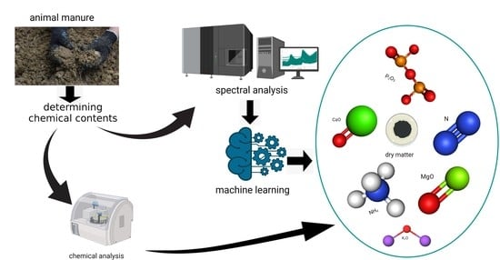
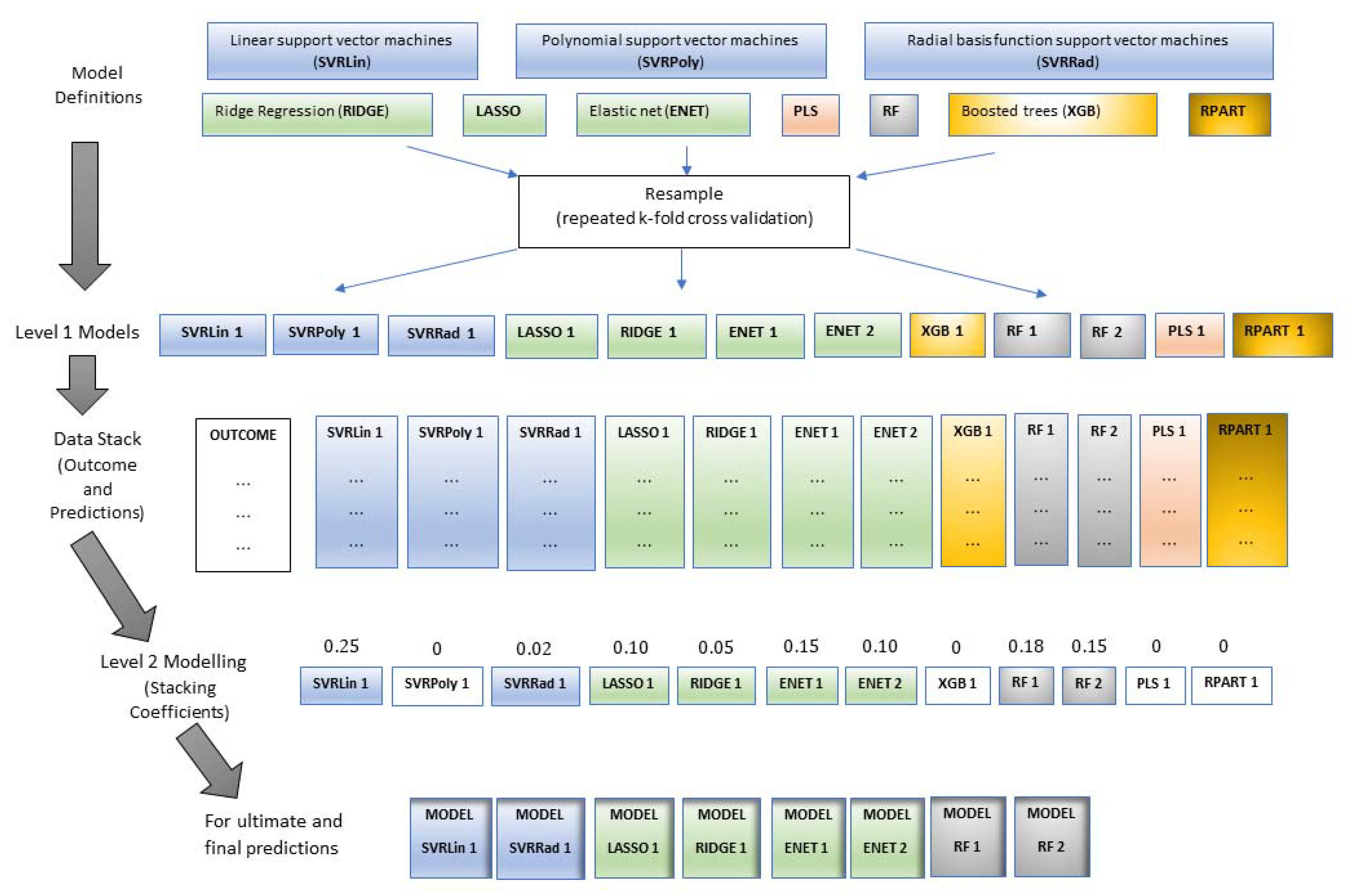
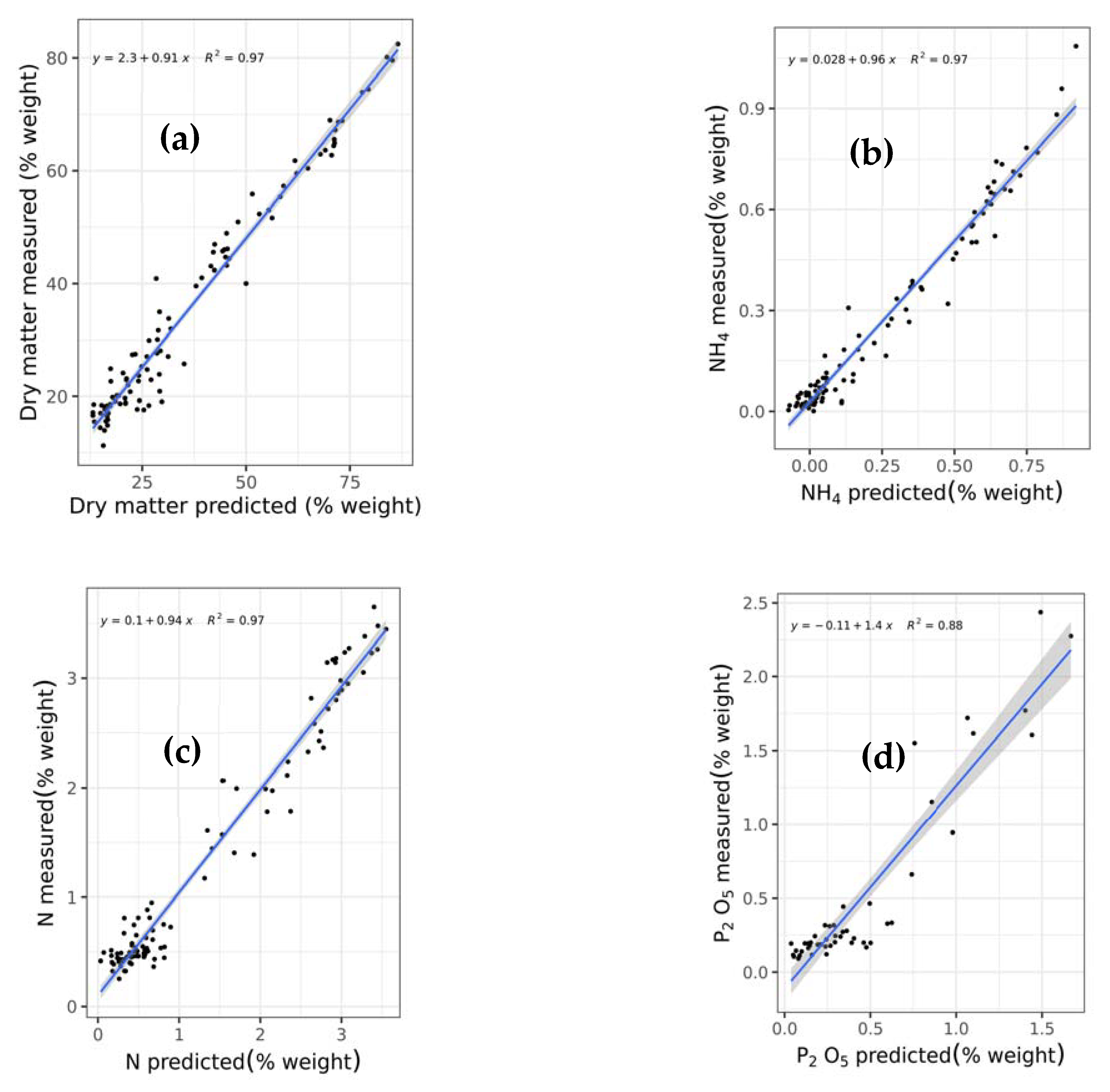
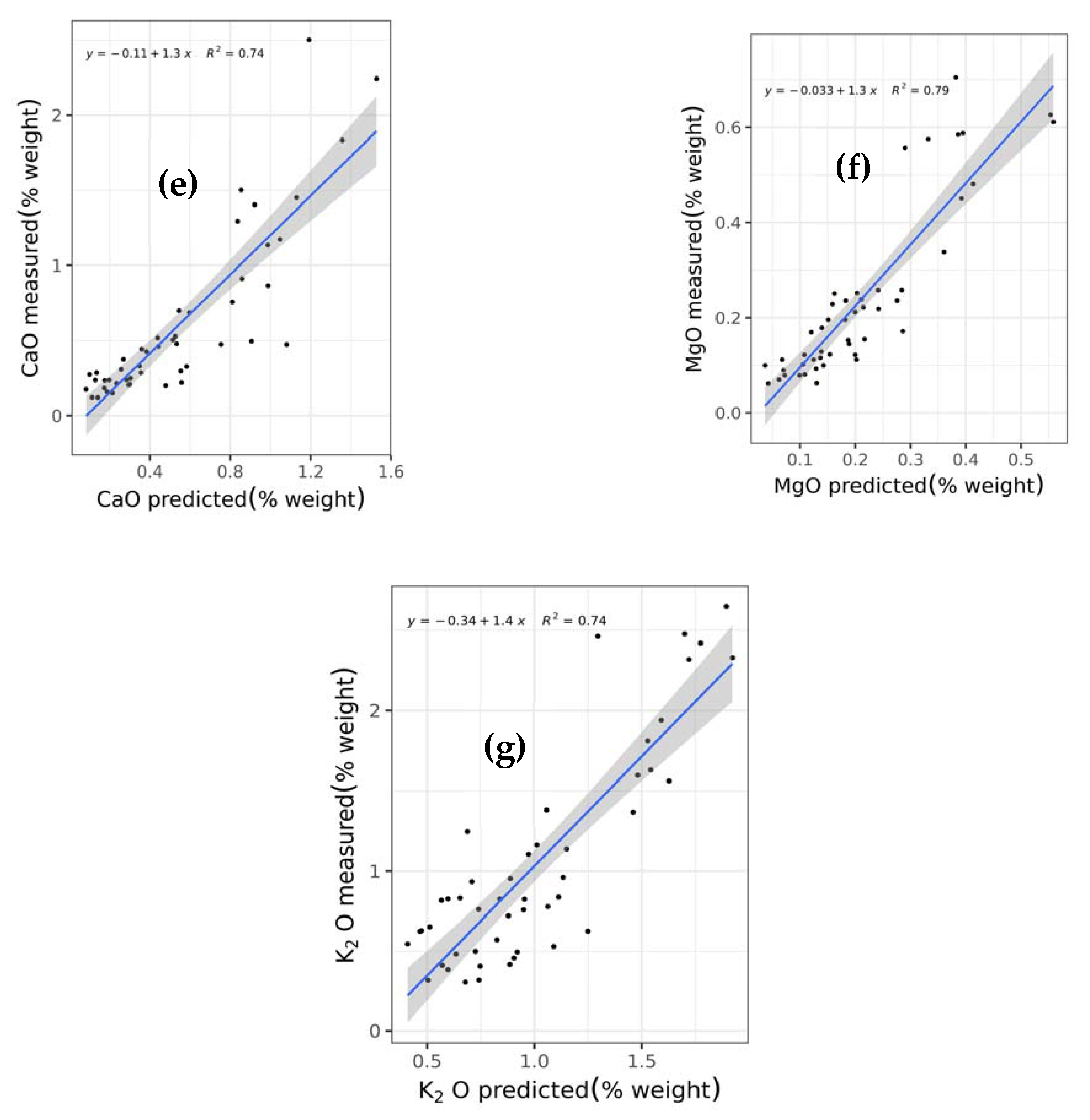
This study is the first to comprehensively compare and test a wide array of machine learning techniques including support vector regression with linear (SVRLin), polynomial (SVRPoly), and radial (SVRRad) basis kernels, LASSO, (RIDGE, elastic net regression (ENET), PLS, RF, recursive partitioning and regression trees (RPART), and boosted trees (XGB) using NIR spectral data, for the simultaneous prediction of seven chemical constituents present in animal manure. These components include dry matter (DM), total ammonium nitrogen (NH4) (designated as NH4 in this study), total N (designated as N in this study), P2O5, CaO, MgO, and K2O. In so doing, we determined the most suitable techniques for the simultaneous determination of the abovementioned chemical components. Results of this study show that stacked regression that collated the performance of the various abovementioned machine learning techniques appears to be a robust machine algorithm for the simultaneous quantification of the seven chemical components in fresh cattle and poultry manure.

2. Materials and Methods

2.1. Dataset

The dataset used in this study was obtained from Gogé et al. and is comprised of 196 cattle and 136 poultry manure samples (a total of 332 samples) collected from livestock production areas in France and Reunion Island. The samples were frozen immediately after collection to prevent any further microbiological activity that causes NH4 losses during storage and were homogenized in the laboratory by crushing them in their frozen state using a blender-cutter (Blixer Dito K45, Electrolux, Senlis, France) [22]. Further details about the materials and reagents, as well as equipment used are provided and explained explicitly in the manuscript by Gogé et al. [22]. A brief explanation of these is provided in the next sections.

2.2. Equipment and Sample Analyses

The NIR spectra were acquired and analyzed on fresh homogenized samples using three different instruments: two XDS Foss (FOSS, Silver Spring, MD, USA) and one NIRFlex Buchi (Flawil, Switzerland) using a rectangular quartz cell (250 mL) (800–2500 nm). The seven chemical properties analyzed include DM, NH4, N, P2O5, CaO, MgO, and K2O. DM, initially at 40 °C, was oven dried at 103 ± 2 °C until it reached a constant weight. Total NH4 and total N were measured by the Kjeldahl method of nitrogen analysis. P2O5, CaO, MgO, and K2O, on the other hand, were measured by ICP (Element XR Thermo Scientific, Waltham, MA, USA) of which only 158 out of 332 samples were analyzed. The descriptive statistics of the different chemical components are summarized in Table 1 [22].
Samples were scanned in triplicate using the abovementioned spectrometers. Each replicated measurement was obtained using the mean of 32 scans. The absorbance was recorded using the equation: absorbance = log(1/reflectance). The final spectrum used in the data analysis was generated using the mean of the triplicate measurements [22].

2.3. Data Preprocessing

The datasets, which are composed of NIR spectra and quantitative results (i.e., concentrations) from various chemical analyses, were split into 232 samples (for DM, NH4, and N) and 110 (for P2O5, CaO, MgO, and K2O) for the training set, and 100 (for DM, NH4, and N) and 48 (for P2O5, CaO, MgO, and K2O) for the test set in a stratified manner based on the type of manure (cattle and poultry manure) so that each of the sets would have the same distribution as the original dataset of cattle and poultry manure before splitting. The rsample package version 1.0.0 in R was used in data splitting [23].
Both the training and test sets were standardized (mean = 0 and standard deviation = 1) separately. The spectra in the training and test sets were further pretreated by Savitzky–Golay smoothing with a differentiation order of 1, polynomial order of 3, window size of 11, and sampling interval of 2 using the prospectr package version 0.2.4 in R [24].
Resampling methods were done on the training set to help understand the effectiveness of the models without touching the test set that we had set aside. Repeated v-fold (or k-fold) cross-validation was used in resampling the training set. The v-fold (or k-fold) cross-validation process worked by further splitting the training set into an analysis set, with each of the v sets containing 1—1/v of the training set (called the “folds”) and 1/v of the training set was set aside for the assessment set. The analysis set was used for modeling, while the assessment set was used to measure the performance of the model. The disadvantage of v-fold (or k-fold) cross-validation is its noisy or high-variability characteristic, and gathering more data helps reduce the noise, but because of the constraints and limitations of collecting more data, cross validation resolves this issue by averaging more than the v statistics. Thus, another fold generation technique is a repeated v-fold (or k-fold) cross-validation in which the v-fold generation process was done R times to create R collections of v partitions, and v × R statistics were used to find the average to estimate the performance of the model. Considering the present size of the training set, a 5-repeat of 10-fold cross-validation was used in this study. For instance, in this study, there were 232 observations (points) for DM, NH4, and N in our training set. The training set was then randomly divided into 10 folds (sometimes called groups) of approximately equal size. Each k-1 (i.e., 9) fold was used for an analysis set and the left out (i.e., 1) fold (i.e., 10% of 232) was used for the assessment (testing) set. With the use of five repeats, there were five groups of 10 or a total of 50 splits created.
Tuning is the process of determining the optimum values of the hyperparameters that cannot be directly determined from the training data and were specified ahead of time. In our study, we used the tuning parameters as shown on Table S1. The grid search method used in this study was just a simple space-filling regular grid of value 100.
Throughout the course of this study, Savitzky–Golay signal filtering was used prior to any data analysis. Savitzky–Golay is a popular smoothing technique based on local least squares fitting of the data by polynomials [25] and can be presented as:
x j = 1 N h = k k c h
where x j is the new value, N is a normalizing coefficient, k is the gap size on each side of j , and c h are pre-computed coefficients that depend on the chosen polynomial order and degree [26,27,28]. All data preprocessing was done on the training and test sets separately to avoid information leakage. No other signal pretreatment methods were used after applying the Savitzky–Golay signal preprocessing technique.

2.4. Individual Machine Learning and Stacked Regression Analyses

This study utilized 10 machine learning regression techniques, namely SVRLin, SVRPoly, SVRRad, LASSO, RIDGE, ENET, PLS, RF, RPART, and XGB. The results of the individual machine learning techniques were then collated using a stacked regression approach. Details about each individual machine learning technique are provided below.
(i)
SVR is a technique in which a model learns a variable’s importance for characterizing the relationship between the input and output. It formulates an optimization problem to learn a regression function that uses the input predictor variables and map these to the output responses. The optimization is represented by using support vectors (i.e., a small set of training data samples) where the optimization solution depends on the number of support vectors instead on the dimension of the input data [26]. Linear (SVRLin), polynomial (SVRPoly), and radial (SVRRad)-basis kernels were utilized in this study. SVR for linear, polynomial, and radial-basis kernels was performed using the ‘kernlab’ package version 0.9.30 in R [27,28].
(ii)
LASSO regression aims to identify the variables and the corresponding regression coefficients leading to a statistical model that minimizes the errors of prediction. This is achieved by imposing a constraint on the model parameters, thus, shrinking the regression coefficients toward zero [29].
(iii)
RIDGE is a popular regression method used to address the issue of collinearity frequently encountered in multiple linear regression techniques [30]. It utilizes a ridge estimator by maximizing the likelihood with a restriction, thus, improving the mean square error [31].
(iv)
ENET provides a bridge between LASSO and RIDGE, thereby improving the prediction accuracy by shrinking some of the regression coefficients to approximately zero as the strength of the penalty parameter increases [32,33]. LASSO, RIDGE, and ENET were conducted using the ‘glmnet’ package version 4.1.2 in R [34,35].
(v)
PLS is a data reduction technique that compresses a large number of measured collinear variables into a few orthogonal latent variables (i.e., principal components). The optimum number of latent variables to be used in the analysis is then determined by minimizing the root mean square error (RMSE) between the predicted and observed response variables [36]. PLS was fitted using the ‘mixOmics’ package version 6.17.26 in R [37]
(vi)
RF builds a predictor ensemble using a set of decision trees that grow in randomly selected subspaces of data [38]. The random sampling and ensemble strategies utilized in this method enable it to achieve predictions and better generalizations [39]. The ‘random forest’ package version 4.7.1.1 in R was used for RF analysis [40].
(vii)
RPART is a regression method often used for the prediction of binary outcomes that avoids the assumptions of linearity [41]. It builds classification or regression models of a very general structure using a two-step process; the resulting models can be represented as binary trees. RPART was performed using the ‘rpart’ package version 4.1.16 in R [42]. RPART was performed using the ‘rpart’ package in R [42].
(viii)
XGB is a highly effective and widely used machine learning technique that combines multiple decision trees to create a more powerful model [43,44]. It builds trees in a serial manner, where each tree tries to correct the mistake of the previous one. Each tree can provide good predictions and, in the process, more and more trees are added to iteratively improve the performance of the predictive model [44]. XGB was conducted using the ‘xgboost’ package version 1.5.1.1 in R [45].
The R packages of the different models listed above were accessed using the R package ‘parsnip’ version 1.0.0 [46] from the ‘tidymodels’ ecosystem [47].’Parsnip’ provides a simple interface to a different range of models in R, whether as core packages or external/separate packages. It provides harmonization on the naming convention of arguments across related models and decoupling of model configurations from the model implementation.
(ix)
Stacked regression is an ensemble learning technique that collates the performance of the abovementioned individual machine learning techniques to optimize model performance [48]. The R package ‘stacks’ version 0.2.3 is part of the tidymodels ecosystem and was used for stacked regression. Individual statistical models (e.g., support vector regression, linear regression (LASSO, RIDGE, and ENET), etc.) were first defined and formed as candidate members (SVRLin1, SVRPoly1, SVRRad1, etc.) of the ensemble (Level 1 models) with each having different parameter values or model configurations in which all of them share the same resampling and repeated k-fold cross-validation. The Level 1 models were then stacked together (data stack) in a tibble format where the first column was the true outcome in the training set and the rest of the columns were the predictions for each candidate member of the ensemble. A regularized model (elastic net) was then fitted on each of the candidate members’ predictions to figure out how they can be combined to predict the true outcome (Level 2 modeling). In this stage, the stacking coefficients were determined with non-zero values retained and became members of the model stack, which were then trained on the full training set. The final model stack was then used to make the final and ultimate predictions on the test set, which was set aside previously, and the performance metrics were then determined (Figure 1).

2.5. Comparative Analysis of the Individual Machine Learning Techniques and Stacked Regression

The performance of all machine learning techniques including that of the stacked regression were both assessed in each of the chemical components in the training and testing sets using the RMSE values, which can be calculated as [49]:
R M S E = i = 1 N ( y i y i ) 2 N
where y and y′ are the predicted and actual concentrations of the chemical constituents, respectively, and N is the number of samples. The root mean square error of cross validation (RMSECV) and the root mean square error of prediction (RMSEP) were both assessed for the training and testing datasets, respectively, using freely available R packages for the aforementioned individual regression techniques. We also assessed the coefficient of determination (R2) for each of the chemical constituents in the training and testing datasets for all machine learning techniques, as well as for that of the stacked regression. The F-test was also used to compare the RMSE values of each individual regression technique at a 95% level of significance. That is, to assess whether the two regression techniques are statistically significantly different, a method was adapted from the previous manuscript published by Payne and Wolfrum [50]. To do this, standard error (SE) values were first calculated between the two machine learning algorithms being compared (i.e., SE = RMSE2)—these are the variance measures. The ratio of these two SE values (i.e., ratio = SE2/SE1) was then determined ensuring a value greater than 1.0. We calculated the critical F-value using the correct number of degrees of freedom (e.g., 231 for DM, NH4, and N; 109 for P2O5, CaO, MgO, and K2O) with a probability confidence level of 0.05. The calculated ratio was then compared with the F-value obtained at a 95% critical level of significance and using the correct number of degrees of freedom, as mentioned. Critical F-value calculations were performed using Free Statistics Calculators version 4.0 [51]. If the obtained ratio is less than the critical F-value, RMSE values are not significantly different. Detailed calculations comparing the ratio of the standard errors of the two different machine learning techniques with that of the critical F-value are provided in Tables S4 and S5.
Another critical parameter used to assess the reliability of the developed statistical model in this study is the ratio of performance to deviation (RPD), which can be expressed as the ratio of the standard deviation to the standard error of prediction. RPD is a widely used statistical parameter that has been commonly used by NIR scientists working on agricultural products [52]. Model reliability was assessed using three different categories including excellent, fair, and non-reliable for RPD > 2, 1.4 < RPD < 2; and RPD < 1.4, respectively [53].

3. Results

3.1. Signal Pretreatment and Descriptive Statistics of the Chemical Components of Poultry and Cattle Manure

A total of 332 fresh homogenized samples were utilized in the study, comprising of 196 cattle manure and 136 poultry manure, as previously indicated. All 332 samples were tested for DM, NH4 and N, while 158 samples were tested for P2O5, CaO, MgO and K2O. The unprocessed NIR spectra of the training and testing set, which plotted absorbance versus wavelength (500–2500 nm) are shown in Figure 2. Savitzky-Golay smoothing was applied for preprocessing to reduce the frequency noise while maintaining relevant spectral information (Figure 3). Similar to the descriptive statistics for the training set (Table 2) and testing set samples (Table 3), the descriptive statistics for the chemical components of the manure samples in percent fresh-weight basis (Table 1) reveal a wide range of values for each chemical constituent.

3.2. Root Mean Square Error of Cross-Validation (RMSECV) and R2 Analyses of the Seven Chemical Components of Fresh Homogenized Samples in the Training Set

Various SVR kernels including linear, polynomial, and radial outperformed all other machine learning techniques in the training set for all chemical components (Table 4 and Table 5). SVRLin performed optimally in MgO and K2O components (RMSECVMgO = 0.074%, R2MgO = 0.786, RMSECVK2O = 0.252%, R2K2O = 0.820), most specifically using the RMSECV parameter. SVRPoly performed optimally well in DM (RMSECVDM = 4.543%, R2DM = 0.946). SVRRad, on the other hand, performed optimally in NH4, N, P2O5, and CaO (RMSECVNH4 = 0.066%, R2NH4 = 0.943, RMSECVN = 0.254%, R2N = 0.946, RMSECVP2O5 = 0.176%, R2P2O5 = 0.849, RMSECVCaO = 0.232%, R2CaO = 0.779) (Table 4 and Table 5). Overall, SVRPoly (RMSECVaverage = 0.817%, R2average = 0.851) and SVRRad (RMSECVaverage = 0.819%, R2average = 0.866) were the best-performing algorithms across all components in the training set. Overall, results of our study show that SVRPoly is not significantly different than that of the other variants of SVR (i.e., SVRLin and SVRRad), LASSO, as well as ENET by comparing the RMSECV values. SVRPoly is not, however, significantly different than that of RIDGE, PLS, RF, RPART, and XGB across all chemical components.
PLS, the traditionally used technique in the NIR analysis did not perform optimally well across all seven chemical components in the training set (RMSECVaverage = 1.182%, R2average = 0.771) (Table 4 and Table 5). RPART (RMSECVaverage = 1.614%, R2average = 0.656) and RIDGE (RMSECVaverage = 1.748%, R2average = 0.736) were the least performing techniques in the training set across all chemical components (Table 4 and Table 5). SVRPoly is not significantly different than that of SVRRad using the RMSECV values for the DM chemical constituent. However, it was found that SVRPoly is significantly different than that of SVRLin and the rest of the other machine learning algorithms in the same chemical component.
For NH4 and CaO, SVRRad is not significantly different than that of SVRPoly but is significantly different than that of SVRLin and all other machine learning techniques. For N, SVRRad is significantly different than that of all other algorithms.
As mentioned earlier, SVRRad is the most optimally performing algorithm for P2O5. The SVRRad for this chemical component was found to be not significantly different than that of SVRLin but is significantly different than that of the rest of the machine learning algorithms. SVRLin is the most optimally performing machine learning technique for MgO and was found to be not significantly different than that of SVRPoly and SVRRad but is significantly different than that of the other machine learning algorithms. Similar to MgO, SVRLin was found to have garnered the most optimally performing algorithm in the training set for K2O. This SVRLin for this chemical constituent is not significantly different than that of the SVRPoly, SVRRad, LASSO, and ENET. However, it is significantly different than that of RIDGE, PLS, RF, RPART, and XGB.

3.3. Root Mean Square Error of Prediction (RMSEP) and R2 Analyses of the Seven Chemical Components of Fresh Homogenized Samples in the Testing Set

To independently assess the performance of the training set, statistical analyses of the testing set data were performed. SVRRad performed optimally well as compared to the other algorithms for the MgO chemical constituent (RMSEPMgO = 0.078%, R2MgO = 0.837) (Table 6 and Table 7).
Stacked regression outperformed all other machine learning techniques in the DM, NH4, N, P2O5, CaO, and K2O chemical constituents (RMSEPDM = 4.088%, R2DM = 0.965, RMSEPNH4 = 0.055%, R2NH4 = 0.966, RMSEPN = 0.217%, R2N = 0.965, RMSEPP2O5 = 0.269%, R2P2O5 = 0.875, RMSEPCaO = 0.309%, R2CaO = 0.743, RMSEPK2O = 0.373%, R2K2O = 0.736) (Table 6 and Table 7). For DM and NH4, stacked regression is significantly different than that of all other machine learning algorithms using the RMSEP values of the aforementioned algorithms. For N, on the other hand, stacked regression was found to be not significantly different than that of SVRRad, but is significantly different than that of all the other machine learning approaches. For P2O5 and MgO, stacked regression was found to be not significantly different than that of SVR kernels, LASSO, ENET, and PLS, but is significantly different than that of RIDGE, RF, RPART, and XGB using their respective RMSEP values.
For CaO, on the other hand, stacked regression, which is the best-performing technique, was found to be not significantly different than that of SVRLin, SVRRad, LASSO, ENET, PLS, RF, and RPART, but is significantly different than that of SVRPoly, RIDGE, and XGB. Lastly, using K2O and across all chemical components, stacked regression was found to be not significantly different than that of all other machine learning algorithms. Using the developed calibration model from the stacked regression, the predicted vs. measured concentrations of the chemical constituents show good linearity in the test set (Figure 4a–g).
It can be observed that comparing the experimentally determined value of K2O in the testing set (i.e., 1.044 % wt) (Table 3) with that of RMSEPK2O by stacked regression (i.e., 0.373 % wt) (Table 6) generated ~36% fluctuations in the K2O. Disparities in the RMSEP values relative to the mean value of the experimentally determined K2O, may be primarily due to the skewed distribution of the K2O chemical measurement results (Figure S10e), as well as the small sample size in the testing set (n = 48). Such disparities in the results could be further improved by taking K2O chemical measurements spanning wide concentration values, as well as increasing the number of samples in the testing set analyses, particularly the poultry manure samples. It should also be noted that during the splitting of the data into training and testing sets, we took into serious consideration an equal distribution of cattle and poultry manure samples in the aforementioned datasets to avoid biases. Such random stratification may lead to a skewed distribution of the K2O chemical measurements leading to fluctuations in the RMSEP values relative to the mean value of the experimentally generated K2O chemical results. This is an inherent disadvantage of data splitting. That is, the predictive accuracy of the model is primarily determined by the function of the resulting sample size as a result of data splitting [54]. Fluctuations in the RMSEP values relative to the mean values of the experimentally determined chemical results for the other components (e.g., P2O5, CaO, and MgO) may probably be explained by the same aforementioned justification (Figure S10d,f,g). It is also worth further exploring and considering the possible limitations of an ICP for the analysis of P2O5, CaO, MgO, and K2O that might lead to the abovementioned disparities in the results. Common limitations of an ICP (i.e., ICP-OES in particular) may include sample drift, poor precision, non-ideal limit of detection, and inaccurate identification that may limit accurate and precise analysis of the analyte of interest [55,56,57,58]. ICP-MS, on the other hand, may suffer from severe matrix effects [59].
While a generally acceptable linearity (R2) can be observed between the stacked regression predicted vs. measured concentrations for most of the chemical constituents, a lower R2 value (i.e., 0.743) for the CaO component was obtained (Table 7). This may be attributed to several factors such as the skewed distribution of the CaO chemical measurement values (Figure S10d), as well as the small sample size in the testing set (n = 48). Thus, as mentioned earlier, this limitation can be improved by increasing the sample size of the testing set data and also expanding the concentration matrices to include a wide range of CaO measured values [54,55,56,57,58,59].

3.4. Ratio of Performance to Deviation (RPD) Analyses of the Testing Test

Based on the RPD analyses, stacked regression generated excellent models for DM, NH4, N, P2O5, and overall across all seven chemical constituents in the testing set (RPDDM = 4.745, RPDNH4 = 5.002, RPDN = 5.062, RPDP2O5 = 2.274, RPDaverage = 3.232) (Table 8). Fair models were obtained, on the other hand, for CaO and K2O using stacked regression (RPDCaO = 1.814, RPDK2O = 1.788). A fair model was also obtained for MgO using ENET (RPDMgO = 1.988). Overall, results using the RPD analyses show that the generated models in the testing set across all chemical components and machine learning techniques can be categorized as either excellent or fair with the stacked regression performing exceptionally robust across all chemical components (RPDaverage = 3.232) (Table 8).

4. Discussion

No studies have comprehensively investigated and compared the role of various machine learning techniques including stacked regression for the simultaneous quantification of DM, NH4, N, P2O5, CaO, MgO, and K2O contents in both cattle and poultry manure collected from livestock production. While previous studies have traditionally utilized a PLS approach for the analysis of the abovementioned chemical constituents using NIR systems [14,60,61], alternative machine learning algorithms may provide better and more accurate results.
Since the optimization of results for this study is highly dependent on the choice of the hyperparameters used, a rigorous and exhaustive grid search approach was used covering an extensive range of values (Table S1). Once hyperparameter values were optimized (Table S2), we then tested and compared the performance of various machine learning techniques.
As shown in this study, PLS, the traditionally used technique in NIR analysis, did not perform fairly well as compared to stacking various machine learning techniques (Table 6, Table 7 and Table 8). While PLS offers several advantages including the ability to handle missing data and intercorrelated predictors, as well as having a robust calibration model, it offers several disadvantages such as difficulty in interpreting loadings of independent variables, as well as that the learned projections are the results of linear combinations of all variables in the independent and dependent datasets, making it challenging to interpret the solutions [62,63,64].
In general, a large number of samples are required to develop a robust calibration model in PLS [65]. In one study, however, a sample size of 100 may be sufficient to achieve acceptable power for moderate effect sizes [66]. While PLS generated an excellent model reliability across all seven chemical constituents (RPDaverage = 2.073) (Table 8), its performance is less superior as compared to the stacked regression technique.
Models with different hyperparameters or configurations were ranked on the basis of their optimum R2 and RMSE values. That is, models (i.e., machine learning algorithms) with the lowest RMSE and highest R2 values were highly ranked (Figures S1–S7). As was evident, PLS was not the top-performing algorithm for each of the chemical components in the workflow rank. The top-performing models were not guaranteed to be included in the Level 2 modeling.
In the stacking procedure implemented in this study, all these models with their corresponding prediction values were stacked together, and a Level 2 model via elastic net was fitted on each of the Level 1 model that became the predictors; stacking coefficients or weights were then determined for each stack member where the only non-zero coefficients were retained to be used for final prediction on the test set (Table S3).
Stacked regression is a very powerful approach that has been successfully applied to a wide array of fields including anticancer drug response prediction, prediction of photosynthetic capacities, image quality assessment, and mortality forecasting, among others [67,68,69,70]. The aforementioned technique has also shown its superior performance in several agricultural applications such as in the estimation of the leaf area index, wild blueberry yield prediction, and crop yield prediction, among others [71,72,73]. However, its particular application in the simultaneous prediction of these seven important chemical components in fresh cattle and poultry manure has not been studied. This study has shown the robust performance of this approach as compared to PLS and other traditionally used machine learning techniques such as SVR (linear, polynomial, and radial), LASSO, RIDGE, ENET, RF, RPART, and XGB. Future studies may consider the effects of various signal preprocessing techniques, as well as wavelength selection strategies for each algorithm prior to stacked regression.

5. Conclusions

Machine learning techniques have proven to be reliable for qualitative and quantitative NIR analysis in a wide range of industries, including agriculture. However, PLS remains the most widely utilized for quantitative prediction of specific sample features. In addition, investigations into the composition of manure have been mostly exclusive to specific components. The results of the current study demonstrate the effectiveness of stacked regression for the simultaneous determination of seven manure chemical components. The technique’s prediction results based on the RPD, RMSEP, and R2 values were evaluated as excellent and outperformed several other machine learning techniques including PLS. Therefore, our study supports the use of stacked regression analysis as a stand-alone technique for analyzing poultry and cattle manure, exhibiting proof-of-principle and superior features amenable to machine learning.

Supplementary Materials

The following supporting information can be downloaded at https://www.mdpi.com/article/10.3390/chemosensors10100410/s1: Figure S1: Workflow rank of the machine learning technique used in the dry matter analysis for the stacked regression; Figure S2: Workflow rank of the machine learning technique used in the total ammonium nitrogen (NH4) analysis for the stacked regression; Figure S3: Workflow rank of the machine learning technique used in the total nitrogen (N) analysis for the stacked regression; Figure S4: Workflow rank of the machine learning technique used in the P2O5 analysis for the stacked regression; Figure S5: Workflow rank of the machine learning technique used in the CaO analysis for the stacked regression; Figure S6: Workflow rank of the machine learning technique used in the MgO analysis for the stacked regression; Figure S7: Workflow rank of the machine learning technique used in the K2O analysis for the stacked regression; Figure S8: Histograms for the 332 samples; Figure S9: Histograms for the 232 samples; Figure S10: Histograms for the 110 samples; Table S1: Ranges of hyperparameters used in tuning of best results for various machine learning techniques. A space-filling design with a grid number of 100 is used. There were 100 equally spaced values between (including) each hyperparameter’s minimum and maximum values that were used for tuning. For hyperparameters that are meaningful only when the values are integers, i.e., the latent variable (LV) in partial least squares (PLS), non-integer values are just skipped during tuning; Table S2: Optimized parameters obtained from different machine learning models; Table S3: The top 10 (or 7) highest weighted (stacking coefficient) members of a stacked ensemble of different models with non-zero coefficients for each of the chemical contents: dry matter (DM), total ammonium nitrogen (NH4), total nitrogen (N), phosphorus pentoxide (P2O5), calcium oxide (CaO), magnesium oxide (MgO), and potassium oxide (K2O); Table S4: Statistical significance table that compares the ratio of the standard errors between two algorithms with that of the critical F-value in the training set; Table S5: Statistical significance table that compares the ratio of the standard errors between two algorithms with that of the critical F-value in the testing set.

Author Contributions

Conceptualization, G.G.D.; methodology, G.G.D., I.A. and O.G.; formal analysis, O.G. and G.G.D.; data curation, O.G. and G.G.D.; writing—original draft preparation, E.C., O.G., I.A., G.G.D., S.K.L. and S.S.; writing—review and editing, I.A., E.C., G.G.D., O.G., S.K.L. and S.S.; visualization, O.G. and G.G.D.; supervision, I.A., G.G.D. and S.S.; project administration, G.G.D.; funding acquisition, G.G.D. All authors have read and agreed to the published version of the manuscript.

Funding

Efforts for this work were made possible through the 2022 US Department of Energy Visiting Professorship Program awarded to Dr. Gerard G. Dumancas. This study was partly funded by the Ministry of Food, Agriculture and Fisheries (CasDar project no. 9109) and ADEME (French Environment and Energy Management Agency). Collection of samples from Reunion Island was partly supported by CIRAD and the Réunion Region (convention no. 20090885) via the European Regional Development Fund. G. Moussard and L. Thuriès were partly supported on Reunion Island by the European Agricultural Fund for Rural Development (FEADER, Measure no. 111.34, Convention no. DEE/20141575); the Conseil Regional de La Réunion; the French Ministry of Agriculture, Food and Fisheries; and CIRAD within the framework of the project “Services et impacts des activités agricoles en milieu tropical” (Siaam).

Data Availability Statement

Data for this analysis was obtained from Gogé, et al. [22] under the CC0—“Public Domain Dedication.”.

Acknowledgments

This research was carried out in part using the Advanced Science and Technology Institute (ASTI) of the Philippine Department of Science and Technology’s (DOST) Computing and Archiving Research Environment (COARE). We would like to thank Thierry Morvan and Youssef Fouad for providing us guidance as we navigate and use their datasets.

Conflicts of Interest

The authors declare no conflict of interest.

References

  1. Farooqi, Z.U.R.; Sabir, M.; Zeeshan, N.; Naveed, K.; Hussain, M.M. Enhancing Carbon Sequestration Using Organic Amendments and Agricultural Practices; IntechOpen: London, UK, 2018; ISBN 978-1-78923-765-8. [Google Scholar]
  2. Rahman, F.; Rahman, M.M.; Rahman, G.K.M.M.; Saleque, M.A.; Hossain, A.T.M.S.; Miah, M.G. Effect of Organic and Inorganic Fertilizers and Rice Straw on Carbon Sequestration and Soil Fertility under a Rice–Rice Cropping Pattern. Carbon Manag. 2016, 7, 41–53. [Google Scholar] [CrossRef]
  3. Bhunia, S.; Bhowmik, A.; Mallick, R.; Mukherjee, J. Agronomic Efficiency of Animal-Derived Organic Fertilizers and Their Effects on Biology and Fertility of Soil: A Review. Agronomy 2021, 11, 823. [Google Scholar] [CrossRef]
  4. Jiaying, M.; Tingting, C.; Jie, L.; Weimeng, F.; Baohua, F.; Guangyan, L.; Hubo, L.; Juncai, L.; Zhihai, W.; Longxing, T.; et al. Functions of Nitrogen, Phosphorus and Potassium in Energy Status and Their Influences on Rice Growth and Development. Rice Sci. 2022, 29, 166–178. [Google Scholar] [CrossRef]
  5. MacDonald, J.M.; Ribaudo, M.; Livingston, M.; Beckman, J.; Huang, W. Manure Use for Fertilizer and for Energy: Report to Congress. Available online: http://www.ers.usda.gov/publications/pub-details/?pubid=42740 (accessed on 23 August 2022).
  6. Khoshnevisan, B.; Duan, N.; Tsapekos, P.; Awasthi, M.K.; Liu, Z.; Mohammadi, A.; Angelidaki, I.; Tsang, D.C.W.; Zhang, Z.; Pan, J.; et al. A Critical Review on Livestock Manure Biorefinery Technologies: Sustainability, Challenges, and Future Perspectives. Renew. Sustain. Energy Rev. 2021, 135, 110033. [Google Scholar] [CrossRef]
  7. Pagliari, P.; Wilson, M.; He, Z. Animal Manure Production and Utilization: Impact of Modern Concentrated Animal Feeding Operations. In ASA Special Publications; Waldrip, H.M., Pagliari, P.H., He, Z., Eds.; American Society of Agronomy, Crop Science Society of America, and Soil Science Society of America: Madison, WI, USA, 2020; pp. 1–14. ISBN 978-0-89118-371-6. [Google Scholar]
  8. Kacprzak, M.; Malińska, K.; Grosser, A.; Sobik-Szołtysek, J.; Wystalska, K.; Dróżdż, D.; Jasińska, A.; Meers, E. Cycles of Carbon, Nitrogen and Phosphorus in Poultry Manure Management Technologies—Environmental Aspects. Crit. Rev. Environ. Sci. Technol. 2022, 1–25. [Google Scholar] [CrossRef]
  9. Peters, J.; Combs, S.; Hoskins, B.; Jarman, J.; Kovar, J.; Watson, M.; Wolf, A.; Wolf, N. Recommended Methods of Manure Analysis; State of Wisconsin Department of Agriculture, Trade and Consumer Protection: Madison, WI, USA, 2003; p. 62.
  10. He, Z.; Pagliari, P.H.; Waldrip, H.M. Applied and Environmental Chemistry of Animal Manure: A Review. Pedosphere 2016, 26, 779–816. [Google Scholar] [CrossRef]
  11. Pagliari, P.H.; Laboski, C.A.M. Investigation of the Inorganic and Organic Phosphorus Forms in Animal Manure. J. Environ. Qual. 2012, 41, 901–910. [Google Scholar] [CrossRef] [PubMed]
  12. Horf, M.; Vogel, S.; Drücker, H.; Gebbers, R.; Olfs, H.-W. Optical Spectrometry to Determine Nutrient Concentrations and Other Physicochemical Parameters in Liquid Organic Manures: A Review. Agronomy 2022, 12, 514. [Google Scholar] [CrossRef]
  13. Horf, M.; Gebbers, R.; Vogel, S.; Ostermann, M.; Piepel, M.-F.; Olfs, H.-W. Determination of Nutrients in Liquid Manures and Biogas Digestates by Portable Energy-Dispersive X-Ray Fluorescence Spectrometry. Sensors 2021, 21, 3892. [Google Scholar] [CrossRef]
  14. Feng, X.; Larson, R.A.; Digman, M.F. Evaluation of Near-Infrared Reflectance and Transflectance Sensing System for Predicting Manure Nutrients. Remote Sens. 2022, 14, 963. [Google Scholar] [CrossRef]
  15. Chen, L.; Xing, L.; Han, L. Review of the Application of Near-Infrared Spectroscopy Technology to Determine the Chemical Composition of Animal Manure. J. Environ. Qual. 2013, 42, 1015–1028. [Google Scholar] [CrossRef]
  16. Roggo, Y.; Chalus, P.; Maurer, L.; Lema-Martinez, C.; Edmond, A.; Jent, N. A Review of near Infrared Spectroscopy and Chemometrics in Pharmaceutical Technologies. J. Pharm. Biomed. Anal. 2007, 44, 683–700. [Google Scholar] [CrossRef]
  17. Kumaravelu, C.; Gopal, A. A Review on the Applications of Near-Infrared Spectrometer and Chemometrics for the Agro-Food Processing Industries. In Proceedings of the 2015 IEEE Technological Innovation in ICT for Agriculture and Rural Development (TIAR), Chennai, India, 10–12 July 2015; pp. 8–12. [Google Scholar]
  18. Huang, G.; Han, L.; Yang, Z.; Wang, X. Evaluation of the Nutrient Metal Content in Chinese Animal Manure Compost Using near Infrared Spectroscopy (NIRS). Bioresour. Technol. 2008, 99, 8164–8169. [Google Scholar] [CrossRef]
  19. Devianti, D.; Sufardi, S.; Mustaqimah, M.; Munawar, A.A. Near Infrared Technology in Agricultural Sustainability: Rapid Prediction of Nitrogen Content from Organic Fertilizer. Transdiscipl. J. Eng. Sci. 2022, 13, 1–12. [Google Scholar] [CrossRef]
  20. Devianti, D.; Yusmanizar, Y.; Syakur, S.; Munawar, A.A.; Yunus, Y. Organic Fertilizer from Agricultural Waste: Determination of Phosphorus Content Using near Infrared Reflectance. OP Conf. Ser. Earth Environ. Sci. 2021, 644, 012002. [Google Scholar] [CrossRef]
  21. Guindo, M.L.; Kabir, M.H.; Chen, R.; Liu, F. Particle Swarm Optimization and Multiple Stacked Generalizations to Detect Nitrogen and Organic-Matter in Organic-Fertilizer Using Vis-NIR. Sensors 2021, 21, 4882. [Google Scholar] [CrossRef] [PubMed]
  22. Gogé, F.; Thuriès, L.; Fouad, Y.; Damay, N.; Davrieux, F.; Moussard, G.; Roux, C.L.; Trupin-Maudemain, S.; Valé, M.; Morvan, T. Dataset of Chemical and Near-Infrared Spectroscopy Measurements of Fresh and Dried Poultry and Cattle Manure. Data Brief 2021, 34, 106647. [Google Scholar] [CrossRef] [PubMed]
  23. Silge, J.; Chow, F.; Kuhn, M.; Wickham, H. Rsample: General Resampling Infrastructure. 2022. Available online: https://rsample.tidymodels.org/ (accessed on 1 August 2022).
  24. Stevens, A.; Ramirez-Lopez, L. An Introduction to the Prospectr Package. 2022. Available online: https://github.com/l-ramirez-lopez/prospectr (accessed on 1 August 2022).
  25. Schmid, M.; Rath, D.; Diebold, U. Why and How Savitzky–Golay Filters Should Be Replaced. ACS Meas. Sci. Au 2022, 2, 185–196. [Google Scholar] [CrossRef]
  26. Zhang, F.; O’Donnell, L.J. Support Vector Regression. In Machine Learning; Elsevier: Amsterdam, The Netherlands, 2020; pp. 123–140. ISBN 978-0-12-815739-8. [Google Scholar]
  27. Karatzoglou, A.; Smola, A.; Hornik, K.; Australia (NICTA), N.I.; Maniscalco, M.A.; Teo, C.H. Kernlab: Kernel-Based Machine Learning Lab. 2022. Available online: https://CRAN.R-project.org/package=kernlab (accessed on 1 August 2022).
  28. Karatzoglou, A.; Smola, A.; Hornik, K.; Zeileis, A. Kernlab-an S4 Package for Kernel Methods in R. J. Stat. Softw. 2004, 11, 1–20. [Google Scholar] [CrossRef] [Green Version]
  29. Ranstam, J.; Cook, J.A. LASSO Regression. Br. J. Surg. 2018, 105, 1348. [Google Scholar] [CrossRef]
  30. McDonald, G.C. Ridge Regression. WIREs Comput. Stat. 2009, 1, 93–100. [Google Scholar] [CrossRef]
  31. Arashi, M.; Saleh, A.K.M.E.; Kibria, B.M.G. Theory of Ridge Regression Estimation with Applications; John Wiley & Sons: Hoboken, NJ, USA, 2019; ISBN 978-1-118-64452-2. [Google Scholar]
  32. Jin, B.; Lorenz, D.A.; Schiffler, S. Elastic-Net Regularization: Error Estimates and Active Set Methods. Inverse Probl. 2009, 25, 115022. [Google Scholar] [CrossRef] [Green Version]
  33. Ciaburro, G. Regression Analysis with R: Design and Develop Statistical Nodes to Identify Unique Relationships within Data at Scale; Packt Publishing Ltd.: Birmingham, UK, 2018; ISBN 978-1-78862-270-7. [Google Scholar]
  34. Friedman, J.H.; Hastie, T.; Tibshirani, R. Regularization Paths for Generalized Linear Models via Coordinate Descent. J. Stat. Softw. 2010, 33, 1–22. [Google Scholar] [CrossRef] [Green Version]
  35. Simon, N.; Friedman, J.H.; Hastie, T.; Tibshirani, R. Regularization Paths for Cox’s Proportional Hazards Model via Coordinate Descent. J. Stat. Softw. 2011, 39, 1–13. [Google Scholar] [CrossRef] [PubMed]
  36. Kassambara, A. Machine Learning Essentials: Practical Guide in R; 2018; ISBN 978-1-986406-85-7. Available online: https://books.google.com.hk/books?hl=zh-TW&lr=&id=745QDwAAQBAJ&oi=fnd&pg=PP2&dq=Machine+Learning+Essentials:+Practical+Guide+in+R+-+Alboukadel+Kassambara+-+Google+Books&ots=5EOsxRV1Mu&sig=CndMacT8zaX4mFhoM25OsMP3eEY&redir_esc=y#v=onepage&q=Machine%20Learning%20Essentials%3A%20Practical%20Guide%20in%20R%20-%20Alboukadel%20Kassambara%20-%20Google%20Books&f=false (accessed on 28 August 2022).
  37. Rohart, F.; Gautier, B.; Singh, A.; Lê Cao, K.-A. MixOmics: An R Package for ‘omics Feature Selection and Multiple Data Integration. PLOS Comput. Biol. 2017, 13, e1005752. [Google Scholar] [CrossRef] [Green Version]
  38. Biau, G. Analysis of a Random Forests Model. J. Mach. Learn. Res. 2012, 13, 33. [Google Scholar]
  39. Qi, Y. Random Forest for Bioinformatics. In Ensemble Machine Learning: Methods and Applications; Zhang, C., Ma, Y., Eds.; Springer: Boston, MA, USA, 2012; pp. 307–323. ISBN 978-1-4419-9326-7. [Google Scholar]
  40. Liaw, A.; Wiener, M. Classification and Regression by RandomForest. Forest 2001, 2, 18–22. [Google Scholar]
  41. Newman, T.B.; Mcculloch, C.E. Statistical Interpretation of Data. In Goldman’s Cecil Medicine; Elsevier: Amsterdam, The Netherlands, 2012; pp. e1–e6. ISBN 978-1-4377-1604-7. [Google Scholar]
  42. Therneau, T.; Atkinson, B.; Port, B.R. (Producer of the initial R.; maintainer 1999–2017) Rpart: Recursive Partitioning and Regression Trees. 2022. Available online: https://cran.r-project.org/web/packages/rpart/ (accessed on 1 August 2022).
  43. Chen, T.; Guestrin, C. XGBoost: A Scalable Tree Boosting System. In Proceedings of the 22nd ACM SIGKDD International Conference on Knowledge Discovery and Data Mining; Association for Computing Machinery, New York, NY, USA, 13–17 August 2016; pp. 785–794. [Google Scholar]
  44. Müller, A.C.; Guido, S. Introduction to Machine Learning with Python: A Guide for Data Scientists; O’Reilly Media, Inc.: Sebastopol, CA, USA, 2016; ISBN 978-1-4493-6989-7. [Google Scholar]
  45. Chen, T.; He, T.; Benesty, M.; Khotilovich, V.; Tang, Y.; Cho, H.; Chen, K.; Mitchell, R.; Cano, I.; Zhou, T.; et al. Xgboost: Extreme Gradient Boosting. 2022. Available online: https://github.com/dmlc/xgboost (accessed on 1 August 2022).
  46. Kuhn, M.; Vaughan, D. Parsnip: A Common API to Modeling and Analysis Functions. 2022. Available online: https://parsnip.tidymodels.org/ (accessed on 1 August 2022).
  47. Kuhn, M.; Vaughan, D. Tidymodels. Available online: https://www.tidymodels.org/ (accessed on 1 August 2022).
  48. Couch, S.P.; Kuhn, M. Stacks: Stacked Ensemble Modeling with Tidy Data Principles. J. Open Source Softw. 2022, 7, 4471. [Google Scholar] [CrossRef]
  49. Faber, N.M. Estimating the Uncertainty in Estimates of Root Mean Square Error of Prediction: Application to Determining the Size of an Adequate Test Set in Multivariate Calibration. Chemom. Intell. Lab. Syst. 1999, 49, 79–89. [Google Scholar] [CrossRef]
  50. Payne, C.E.; Wolfrum, E.J. Rapid Analysis of Composition and Reactivity in Cellulosic Biomass Feedstocks with Near-Infrared Spectroscopy. Biotechnol. Biofuels 2015, 8, 43. [Google Scholar] [CrossRef] [Green Version]
  51. Free Critical F-Value Calculator—Free Statistics Calculators. Available online: https://www.danielsoper.com/statcalc/calculator.aspx?id=4 (accessed on 23 August 2022).
  52. Murphy, D.J.; O’Brien, B.; O’Donovan, M.; Condon, T.; Murphy, M.D. A near Infrared Spectroscopy Calibration for the Prediction of Fresh Grass Quality on Irish Pastures. Inf. Process. Agric. 2022, 9, 243–253. [Google Scholar] [CrossRef]
  53. Chang, C.-W.; Laird, D.A.; Mausbach, M.J.; Hurburgh, C.R., Jr. Near-Infrared Reflectance Spectroscopy–Principal Components Regression Analyses of Soil Properties. Soil Sci. Soc. Am. J. 2001, 65, 480–490. [Google Scholar] [CrossRef]
  54. Ette, E.I.; Williams, P.J. Pharmacometrics: The Science of Quantitative Pharmacology; John Wiley & Sons: Hoboken, NJ, USA, 2013; ISBN 978-1-118-67951-7. [Google Scholar]
  55. Levine, M. The Strengths and Limitations of ICP-OES Analysis. Available online: https://www.analyticalcannabis.com/articles/icp-oes-icp-chemistry-icp-oes-analysis-strengths-and-limitations-312835 (accessed on 28 August 2022).
  56. Nizio, K.D.; Harynuk, J.J. Analysis of Alkyl Phosphates in Petroleum Samples by Comprehensive Two-Dimensional Gas Chromatography with Nitrogen Phosphorus Detection and Post-Column Deans Switching. J. Chromatogr. A 2012, 1252, 171–176. [Google Scholar] [CrossRef] [PubMed]
  57. Merson, S.; Evans, P. A High Accuracy Reference Method for the Determination of Minor Elements in Steel by ICP-OES. J. Anal. At. Spectrom. 2003, 18, 372–375. [Google Scholar] [CrossRef]
  58. Jantzi, S.C.; Motto-Ros, V.; Trichard, F.; Markushin, Y.; Melikechi, N.; De Giacomo, A. Sample Treatment and Preparation for Laser-Induced Breakdown Spectroscopy. Spectrochim. Acta Part B At. Spectrosc. 2016, 115, 52–63. [Google Scholar] [CrossRef]
  59. Olesik, J. ICP-OES Capabilities, Developments, Limitations, and Any Potential Challengers? Spectroscopy 2020, 35, 18–21. [Google Scholar]
  60. Gogé, F.; Thuriès, L.; Fouad, Y.; Damay, N.; Davrieux, F.; Moussard, G.; Roux, C.L.; Trupin-Maudemain, S.; Valé, M.; Morvan, T. Performance of near Infrared Spectroscopy of a Solid Cattle and Poultry Manure Database Depends on the Sample Preparation and Regression Method Used. J. Near Infrared Spectrosc. 2021, 29, 226–235. [Google Scholar] [CrossRef]
  61. Xing, L.; Chen, L.J.; Han, L.J. Rapid Analysis of Layer Manure Using Near-Infrared Reflectance Spectroscopy. Poult. Sci. 2008, 87, 1281–1286. [Google Scholar] [CrossRef]
  62. Pirouz, D.M. An Overview of Partial Least Squares. SSRN Electron. J. 2006, 1–16. [Google Scholar] [CrossRef] [Green Version]
  63. Trygg, J.; Wold, S. O2-PLS, a Two-Block (X-Y) Latent Variable Regression (LVR) Method with an Integral OSC Filter. J. Chemom. 2003, 17, 53–64. [Google Scholar] [CrossRef]
  64. Xia, Y. Chapter Eleven—Correlation and Association Analyses in Microbiome Study Integrating Multiomics in Health and Disease. In Progress in Molecular Biology and Translational Science; Sun, J., Ed.; The Microbiome in Health and Disease; Academic Press: Cambridge, MA, USA, 2020; Volume 171, pp. 309–491. [Google Scholar]
  65. Solomon, K.R.; Brock, T.C.M.; Zwart, D.D.; Dyer, S.D.; Posthuma, L.; Richards, S.; Sanderson, H.; Sibley, P.; van den Brink, P.J. Extrapolation Practice for Ecotoxicological Effect Characterization of Chemicals; CRC Press: Boca Raton, FL, USA, 2008; ISBN 978-1-4200-7392-8. [Google Scholar]
  66. Willaby, H.W.; Costa, D.S.J.; Burns, B.D.; MacCann, C.; Roberts, R.D. Testing Complex Models with Small Sample Sizes: A Historical Overview and Empirical Demonstration of What Partial Least Squares (PLS) Can Offer Differential Psychology. Pers. Individ. Differ. 2015, 84, 73–78. [Google Scholar] [CrossRef]
  67. Su, R.; Liu, X.; Xiao, G.; Wei, L. Meta-GDBP: A High-Level Stacked Regression Model to Improve Anticancer Drug Response Prediction. Brief. Bioinform. 2020, 21, 996–1005. [Google Scholar] [CrossRef] [PubMed]
  68. Fu, P.; Meacham-Hensold, K.; Guan, K.; Bernacchi, C.J. Hyperspectral Leaf Reflectance as Proxy for Photosynthetic Capacities: An Ensemble Approach Based on Multiple Machine Learning Algorithms. Front. Plant Sci. 2019, 10, 730. [Google Scholar] [CrossRef]
  69. Zhang, K.; Zhu, D.; Li, J.; Gao, X.; Gao, F.; Lu, J. Learning Stacking Regression for No-Reference Super-Resolution Image Quality Assessment. Signal Process. 2021, 178, 107771. [Google Scholar] [CrossRef]
  70. Kessy, S.R.; Sherris, M.; Villegas, A.M.; Ziveyi, J. Mortality Forecasting Using Stacked Regression Ensembles. Scand. Actuar. J. 2021, 2022, 591–626. [Google Scholar] [CrossRef]
  71. Cheng, Q.; Xu, H.; Fei, S.; Li, Z.; Chen, Z. Estimation of Maize LAI Using Ensemble Learning and UAV Multispectral Imagery under Different Water and Fertilizer Treatments. Agriculture 2022, 12, 1267. [Google Scholar] [CrossRef]
  72. Seireg, H.R.; Omar, Y.M.K.; El-Samie, F.E.A.; El-Fishawy, A.S.; Elmahalawy, A. Ensemble Machine Learning Techniques Using Computer Simulation Data for Wild Blueberry Yield Prediction. IEEE Access 2022, 10, 64671–64687. [Google Scholar] [CrossRef]
  73. Anbananthen, K.S.M.; Subbiah, S.; Chelliah, D.; Sivakumar, P.; Somasundaram, V.; Velshankar, K.H.; Khan, M.K.A.A. An Intelligent Decision Support System for Crop Yield Prediction Using Hybrid Machine Learning Algorithms. F1000Research 2021, 10, 1143. [Google Scholar] [CrossRef]
Figure 1. The visual outline of the steps in stack regression. The models were first defined in which each Level 1 model has different parameter values. The models with different configurations were then stacked together and a regularized model was then fitted on each of the candidate members to determine which members have non-zero coefficients that are to be used for final and ultimate predictions (SVRLin = support vector regression with linear kernel; SVRPoly = support vector regression with polynomial kernel; SVRRad = support vector regression with radial kernel; LASSO = least absolute shrinkage and selection operator; RIDGE = ridge regression; ENET = elastic net regression; PLS = partial least squares; RF = random forests; RPART = recursive partitioning and regression trees; XGB = boosted trees) [48].
Chemosensors 10 00410 g001
Figure 2. Near-infrared spectra of fresh homogenized cattle and poultry manure samples as shown in different line colors.
Chemosensors 10 00410 g002
Figure 3. Near-infrared spectra after standardization (mean = 0, standard deviation = 1) and Savitzky-Golay smoothing of fresh homogenized cattle and poultry manure samples as shown in different line colors.
Chemosensors 10 00410 g003
Figure 4. Predicted vs. measured concentrations of chemical constituents expressed as % wet weight of the fresh cattle and poultry manure for (a) dry matter, (b) total ammonium nitrogen (NH4), (c) total nitrogen (N), (d) P2O5, (e) CaO, (f) MgO, and (g) K2O using the stacked regression ensemble approach.
Chemosensors 10 00410 g004aChemosensors 10 00410 g004b
Table 1. Descriptive statistics of the chemical components of poultry and cattle manure in fresh-weight basis (%) (n = number of samples, sd = standard deviation, min = minimum value, max = maximum value).
ChemicalsnMeanMediansdMinMax
DM33237.28527.88520.06311.25582.480
NH43320.2620.0950.2760.0011.086
N3321.3690.6721.0930.2554.152
P2O51580.4770.2240.5850.0913.020
CaO1580.5750.3300.5560.0943.108
MgO1580.2270.1560.1860.0621.054
K2O1581.0220.8260.6480.1873.845
Table 2. Descriptive statistics of the chemical components of poultry and cattle manure in fresh-weight basis (%) of the 232 (for dry matter (DM), total ammonium nitrogen (NH4), and total nitrogen (N)) and 110 (for P2O5, CaO, MgO, and K2O) samples for the training set. (n = number of samples, sd = standard deviation, min = minimum value, max = maximum value.)
ChemicalsnMeanMediansdMinMax
DM23238.03528.97220.34012.69081.990
NH42320.2620.0910.2770.0010.968
N2321.3840.6751.0920.3114.152
P2O51100.4680.2250.5750.0983.020
CaO1100.5630.3290.5560.0943.108
MgO1100.2220.1470.1900.0681.054
K2O1101.0130.8620.6420.1873.845
Table 3. Descriptive statistics of the chemical components of poultry and cattle manure in fresh-weight basis (%) of the 100 (for dry matter (DM), total ammonium nitrogen (NH4), and total nitrogen (N)) and 48 (for P2O5, Cao, MgO, and K2O) samples for the test set, which are then set aside for the final arbitration on the performance of the different models. (n = number of samples, sd = standard deviation, min = minimum value, max = maximum value.)
ChemicalsnMeanMediansdMinMax
DM10035.54627.24019.39611.25582.480
NH41000.2620.1050.2760.0011.086
N1001.3340.6631.0990.2553.650
P2O5480.4970.2110.6120.0912.437
CaO480.6020.4010.5610.1202.503
MgO480.2370.1760.1790.0620.705
K2O481.0440.8250.6680.3072.649
Table 4. Comparison of the root mean square error of cross validation (RMSECV) (% wet weight) among the seven chemical components (i.e., dry matter (DM), total ammonium nitrogen (NH4), total nitrogen (N), P2O5, CaO, MgO, and K2O) of the fresh homogenized samples using various machine learning techniques (SVRLin = support vector regression with linear kernel; SVRPoly = support vector regression with polynomial kernel; SVRRad = support vector regression with radial kernel; LASSO = least absolute shrinkage and selection operator; RIDGE = ridge regression; ENET = elastic net regression; PLS = partial least squares; RF = random forests; RPART = recursive partitioning and regression trees; XGB = boosted trees). Best results are indicated in bold.
AlgorithmDMNH4NP2O5CaOMgOK2OAverage
SVRLin5.4610.0770.2910.1980.3000.0740.2520.950
SVRPoly4.5430.0700.2960.2070.2640.0770.2580.817
SVRRad4.6560.0660.2540.1760.2320.0790.2690.819
LASSO5.9300.0870.3150.2180.3130.0900.2831.034
RIDGE10.1890.1280.5360.2890.3640.1080.6241.748
ENET5.9280.0870.3150.2180.3120.0890.2841.033
PLS6.7870.0930.3870.2560.3520.1060.2961.182
RF6.8800.0920.3800.2850.3170.0930.3481.199
RPART9.3380.1260.5400.3730.3650.1120.4461.614
XGB5.6830.0820.3460.2430.3030.0920.3261.011
Table 5. Comparison of R2 in the training set among the seven chemical components: dry matter (DM), total ammonium nitrogen (NH4), total nitrogen (N), P2O5, CaO, MgO, and K2O of the fresh homogenized samples using various machine learning techniques (SVRLin = support vector regression with linear kernel; SVRPoly = support vector regression with polynomial kernel; SVRRad = support vector regression with radial kernel; LASSO = least absolute shrinkage and selection operator; RIDGE = ridge regression; ENET = elastic net regression; PLS = partial least squares; RF = random forests; RPART = recursive partitioning and regression trees; XGB = boosted trees). Best results are indicated in bold.
AlgorithmDMNH4NP2O5CaOMgOK2OAverage
SVRLin0.9230.9220.9300.8180.6610.7860.8200.837
SVRPoly0.9460.9370.9280.8170.7130.8060.8100.851
SVRRad0.9450.9430.9460.8490.7790.8170.7830.866
LASSO0.9100.9000.9180.7960.6520.7430.7760.814
RIDGE0.7950.8130.8010.7480.5900.6840.7200.736
ENET0.9100.9010.9180.7970.6530.7480.7750.815
PLS0.8850.8910.8790.7330.5860.6750.7490.771
RF0.8750.8860.8800.7290.6480.7620.6950.782
RPART0.7750.7890.7570.5840.5290.6450.5090.656
XGB0.9170.9110.8990.7700.6720.7480.7210.805
Table 6. Comparison of the root mean square error of prediction (RMSEP) (% wet weight) among the seven chemical components: dry matter (DM), total ammonium nitrogen (NH4), total nitrogen (N), P2O5, CaO, MgO, and K2O of the fresh homogenized samples using various machine learning techniques (SVRLin = support vector regression with linear kernel; SVRPoly = support vector regression with polynomial kernel; SVRRad = support vector regression with radial kernel; LASSO = least absolute shrinkage and selection operator; RIDGE = ridge regression; ENET = elastic net regression; PLS = partial least squares; RF = random forests; RPART = recursive partitioning and regression trees; XGB = boosted trees). Best results are indicated in bold.
AlgorithmDMNH4NP2O5CaOMgOK2OAverage
SVRLin6.9090.0750.3430.3060.3220.0960.3991.207
SVRPoly5.1580.0780.3460.3070.4100.0910.3980.970
SVRRad5.0050.0910.2520.2750.3730.0780.3740.921
LASSO7.1540.0820.3680.3170.3350.0910.4121.251
RIDGE9.3070.1020.5050.3900.3940.1070.4721.611
ENET7.1030.0830.3700.3170.3350.0900.4121.244
PLS8.6470.0970.4490.3200.3490.0920.4411.485
RF5.9870.0910.3390.4490.3800.1210.4711.120
RPART11.2840.1300.5660.5070.3770.1450.4661.925
XGB5.6420.0820.2790.4580.4070.1330.4141.059
Stack Reg4.0880.0550.2170.2690.3090.0920.3730.772
Table 7. Comparison of the R2 in the testing set among the seven chemical components: dry matter (DM), total ammonium nitrogen (NH4), total nitrogen (N), P2O5, CaO, MgO, and K2O of the fresh homogenized samples using various machine learning techniques (SVRLin = support vector regression with linear kernel; SVRPoly = support vector regression with polynomial kernel; SVRRad = support vector regression with radial kernel; LASSO = least absolute shrinkage and selection operator; RIDGE = ridge regression; ENET = elastic net regression; PLS = partial least squares; RF = random forests; RPART = recursive partitioning and regression trees; XGB = boosted trees). Best results are indicated in bold.
AlgorithmDMNH4NP2O5CaOMgOK2OAverage
SVRLin0.9190.9440.9280.7700.6730.7160.6560.801
SVRPoly0.9480.9460.9240.7720.4700.7660.6580.783
SVRRad0.9500.8960.9510.8520.5640.8370.6890.820
LASSO0.8920.9240.9000.7810.6490.7610.6240.790
RIDGE0.8120.8680.8080.6600.5270.6780.5170.696
ENET0.8940.9230.8990.7810.6480.7710.6240.792
PLS0.8390.8940.8510.7420.6110.7480.5570.749
RF0.9150.8970.9130.5680.6760.7090.6770.765
RPART0.6830.7870.7520.3510.5940.4330.5390.591
XGB0.9240.9160.9370.6580.5520.6120.7290.761
Stack Reg0.9650.9660.9650.8750.7430.7920.7360.863
Table 8. Comparison of the ratio of performance to deviation (RPD) in the testing set among the seven chemical components: dry matter (DM), total ammonium nitrogen (NH4), total nitrogen (N), P2O5, CaO, MgO and K2O of the fresh homogenized samples using various machine learning techniques (SVRLin = support vector regression with linear kernel; SVRPoly = support vector regression with polynomial kernel; SVRRad = support vector regression with radial kernel; LASSO = least absolute shrinkage and selection operator; RIDGE = ridge regression; ENET = elastic net regression; PLS = partial least squares; RF = random forests; RPART = recursive partitioning and regression trees; XGB = boosted trees). Best results are indicated in bold.
AlgorithmDMNH4NP2O5CaOMgOK2OAverage
SVRLin2.8073.5453.2022.0001.7451.8551.6742.404
SVRPoly3.7613.5453.1751.9931.3701.9651.6762.498
SVRRad3.8753.0424.3552.2231.5032.2931.7832.725
LASSO2.7113.3572.9851.9311.6771.9621.6212.321
RIDGE2.0842.7042.1751.5701.4231.6641.4151.862
ENET2.7313.3482.9731.9301.6751.9881.6202.324
PLS2.2432.8412.4501.9131.6091.9381.5142.073
RF3.2403.0543.2411.3631.4751.4781.4172.181
RPART1.7192.1241.9421.2081.4871.2361.4321.593
XGB3.4383.3573.9431.3361.3801.3471.6122.345
Stack Reg4.7455.0025.0622.2741.8141.9381.7883.232
Publisher’s Note: MDPI stays neutral with regard to jurisdictional claims in published maps and institutional affiliations.

