Prediction of Type 2 Diabetes Risk and Its Effect Evaluation Based on the XGBoost Model


Abstract
1. Introduction
2. Materials and Methods
2.1. Experimental Data
2.2. Feature Vectors Representation
2.3. EXtreme Gradient Boosting Algorithm
- 1.
- Before starting to iterate the new tree, calculate the first and second derivative matrices of the loss function corresponding to each sample.
- 2.
- Each iteration adds a new tree, and each tree fits the residual of the previous tree.
- 3.
- Count the split gain value of the objective function to select the best split point, and employ the greedy algorithm to determine the best structure of the tree.
- 4.
- Add a new tree to the model and multiply it by a factor to prevent overfitting. When fitting residuals, step size or learning rate are usually used to control optimization, so as to reserve more optimization space for subsequent learning.
- 5.
- After training, a model of multiple trees is obtained, in which each tree has multiple leaf nodes.
- 6.
- In each tree, the sample falls on several leaf nodes according to the eigenvalues. The final predicted value is the score of the leaf node corresponding to each tree multiplied by the weight of the tree.
2.4. Baseline Algorithms
2.5. Parameters Adjustment
2.6. Statistical Analysis
3. Results
3.1. Statistics Results
3.2. Training and Testing Sets Distribution
3.3. Models Comparison
3.3.1. XGBoost Model Results
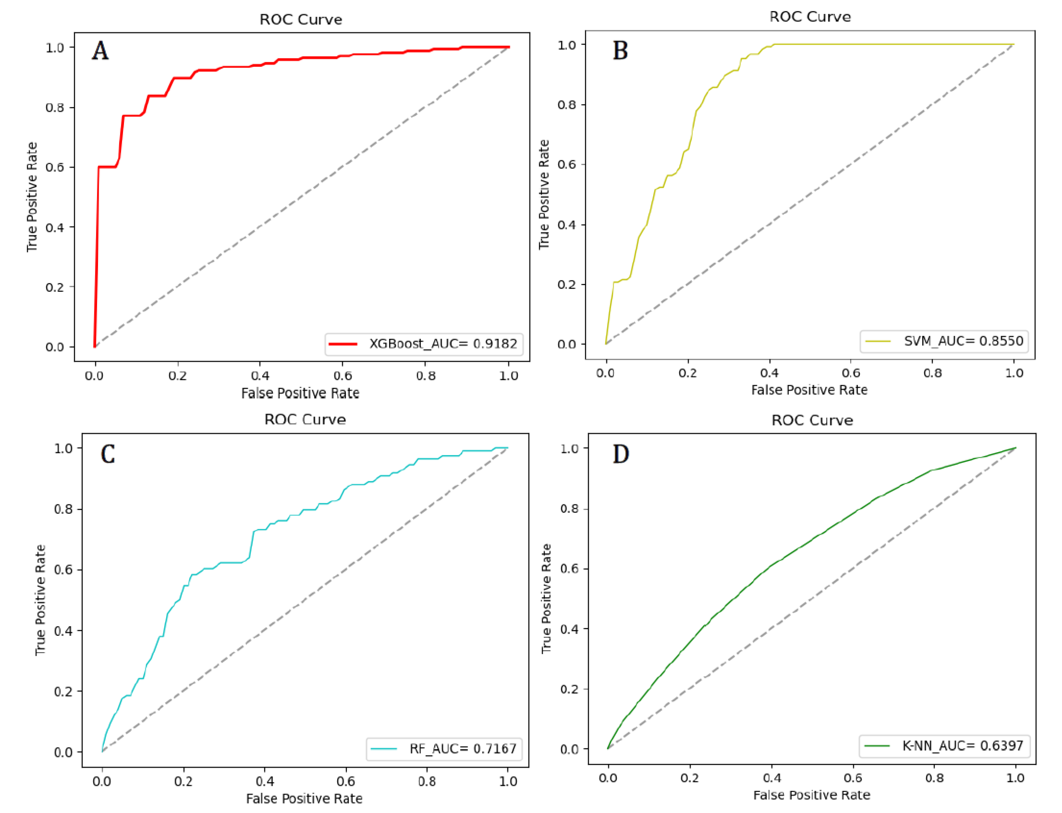
3.3.2. Comparison with Baseline
3.4. Diabetes Risk Prediction
4. Discussion
5. Conclusions
Author Contributions
Funding
Conflicts of Interest
References
- Ahola, A.J.; Groop, P.-H. Barriers to self-management of diabetes. Diabet. Med. 2013, 30, 413–420. [Google Scholar] [CrossRef] [PubMed]
- Wang, Q.; Zhang, X.; Fang, L.; Guan, Q.; Guan, L.; Li, Q. Prevalence, awareness, treatment and control of diabetes mellitus among middle-aged and elderly people in a rural Chinese population: A cross-sectional study. PLoS ONE 2018, 13, e0198343. [Google Scholar] [CrossRef] [PubMed]
- Jen, C.-H.; Wang, C.-C.; Jiang, B.C.; Chu, Y.-H.; Chen, M.-S. Application of classification techniques on development an early-warning system for chronic illnesses. Expert Syst. Appl. 2012, 39, 8852–8858. [Google Scholar] [CrossRef]
- Farwell, W.R.; Gaziano, J.M.; Norkus, E.P.; Sesso, H.D. The Relationship between Total Plasma Carotenoids and Risk Factors for Chronic Disease among Middle-Aged and Older Men. Br. J. Nutr. 2008, 100, 883–889. [Google Scholar] [CrossRef] [PubMed]
- Finkelstein, J.; Jeong, I.C. Machine learning approaches to personalize early prediction of asthma exacerbations. Ann. N. Y. Acad. Sci. 2017, 1387, 153–165. [Google Scholar] [CrossRef] [PubMed]
- Park, J.; Edington, D.W. A sequential neural network model for diabetes prediction. Artif. Intell. Med. 2001, 23, 277–293. [Google Scholar] [CrossRef]
- Zhu, C.-S.; Idemudia, C.U.; Feng, W. Improved logistic regression model for diabetes prediction by integrating PCA and K-means techniques. Inform. Med. Unlocked 2019, 17. [Google Scholar] [CrossRef]
- Sudharsan, B.; Peeples, M.; Shomali, M. Hypoglycemia Prediction Using Machine Learning Models for Patients with Type 2 Diabetes. J. Diabetes Sci. Technol. 2014, 9, 86–90. [Google Scholar] [CrossRef] [PubMed]
- Zhang, D.; Qian, L.; Mao, B.; Huang, C.; Huang, B.; Si, Y. A Data-Driven Design for Fault Detection of Wind Turbines Using Random Forests and XGBoost. IEEE Access 2018, 6, 21020–21031. [Google Scholar] [CrossRef]
- Li, C.; Zheng, X.; Yang, Z.; Kuang, L. Predicting Short-Term Electricity Demand by Combining the Advantages of ARMA and XGBoost in Fog Computing Environment. Wirel. Commun. Mob. Comput. 2018, 2018, 5018053. [Google Scholar] [CrossRef]
- Dhaliwal, S.; Nahid, A.A.; Abbas, R. Effective Intrusion Detection System Using XGBoost. Information 2018, 9, 149. [Google Scholar] [CrossRef]
- Dong, H.; Xu, X.; Wang, L.; Pu, F. Gaofen-3 PolSAR Image Classification via XGBoost and Polarimetric Spatial Information. Sensors 2018, 18, 611. [Google Scholar] [CrossRef] [PubMed]
- Abdullah, N.; Murad, N.A.; Hanif, E.A.M.; Syafruddin, S.E.; Attia, J.; Oldmeadow, C.; Kamaruddin, M.; Jalal, N.A.; Ismail, N.; Ishak, M.; et al. Predicting type 2 diabetes using genetic and environmental risk factors in a multi-ethnic Malaysian cohort. Public Health 2017, 149, 31–38. [Google Scholar] [CrossRef] [PubMed]
- Murugan, A.; Nair, S.A.H.; Kumar, K.P.S. Detection of Skin Cancer Using SVM, Random Forest and kNN Classifiers. J. Med. Syst. 2019, 43, 269. [Google Scholar] [CrossRef] [PubMed]
- Ang, J.C.; Haron, H.; Hamed, H.N.A. Semi-supervised SVM-based Feature Selection for Cancer Classification using Microarray Gene Expression Data. In Current Approaches in Applied Artificial Intelligence; Springer: Cham, Switzerland, 2005; Volume 9101, pp. 468–477. [Google Scholar]
- Zhao, C.; Zhang, H.; Zhang, X.; Liu, M.; Hu, Z.; Fan, B. Application of Support Vector Machine (SVM) for Prediction Toxic Activity of Different Data Sets. Toxicology 2006, 217, 105–119. [Google Scholar] [CrossRef] [PubMed]
- Xiong, X.-L.; Zhang, R.-X.; Bi, Y.; Zhou, W.-H.; Yu, Y.; Zhu, D. Machine Learning Models in Type 2 Diabetes Risk Prediction: Results from a Cross-sectional Retrospective Study in Chinese Adults. Curr. Med Sci. 2019, 39, 582–588. [Google Scholar] [CrossRef] [PubMed]
- López, B.; Torrent-Fontbona, F.; Viñas, R.; Fernandez-Real, J.-M. Single Nucleotide Polymorphism relevance learning with Random Forests for Type 2 diabetes risk prediction. Artif. Intell. Med. 2018, 85, 43–49. [Google Scholar] [CrossRef] [PubMed]
- Nai-Arun, N.; Moungmai, R. Comparison of Classifiers for the Risk of Diabetes Prediction. Procedia Comput. Sci. 2015, 69, 132–142. [Google Scholar] [CrossRef]
- Zhong, J.; Sun, Y.; Peng, W.; Xie, M.; Yang, J.; Tang, X. XGBFEMF: An XGBoost-based Framework for Essential Protein Prediction. IEEE Trans. NanoBiosci. 2018, 17, 243–250. [Google Scholar] [CrossRef] [PubMed]


| Parameter Name | Value |
|---|---|
| gamma | 0.1 |
| max_depth | 0.5 |
| lambda | 3.0 |
| subsample | 0.7 |
| silent | 1.0 |
| eta | 0.1 |
| seed | 1000.0 |
| Parameter Name | Value |
|---|---|
| C | 1.0 |
| degree | 3.0 |
| epsilon | 0.2 |
| gamma | auto |
| tol | 0.001 |
| Parameter Name | Value |
|---|---|
| n_estimators | 60 |
| max_depth | 13 |
| max_features | 9 |
| Random_state | 20 |
| oob_score | True |
| Parameter Name | Value |
|---|---|
| n_neighbors | 5 |
| n_jobs | 1 |
| Type of Information | Classification | Number of People (Individual) | Proportion (%) | |
|---|---|---|---|---|
| Personal Information | Education Level | High Educational Background | 237 | 64.40 |
| High School Degree or Even Lower | 131 | 35.60 | ||
| Marriage | Married | 304 | 82.61 | |
| Unmarried | 64 | 17.39 | ||
| Eating Habits | Rice | Three Times a Day or Even More | 324 | 88.04 |
| Twice a Day | 20 | 5.43 | ||
| Once a Day or Even Not | 24 | 6.52 | ||
| Buns | Three Times a Day or Even More | 312 | 84.78 | |
| Twice a Day | 32 | 8.70 | ||
| Once a Day or Even Not | 24 | 6.52 | ||
| Noodles | Three Times a Day or Even More | 38 | 10.33 | |
| Twice a Day | 67 | 18.21 | ||
| Once a Day or Even Not | 263 | 71.47 | ||
| Pork | Three Times a Day or Even More | 156 | 42.39 | |
| Twice a Day | 127 | 34.51 | ||
| Once a Day or Even Not | 85 | 23.10 | ||
| Beef | Three Times a Day or Even More | 120 | 32.61 | |
| Twice a Day | 93 | 25.27 | ||
| Once a Day or Even Not | 155 | 42.12 | ||
| Fish | Three Times a Day or Even More | 145 | 39.40 | |
| Twice a Day | 129 | 35.05 | ||
| Once a Day or Even Not | 94 | 25.54 | ||
| Seafood | Three Times a Day or Even More | 31 | 8.42 | |
| Twice a Day | 54 | 14.67 | ||
| Once a Day or Even Not | 283 | 76.90 | ||
| Dairy Products | Three Times a Day or Even More | 62 | 16.85 | |
| Twice a Day | 88 | 23.91 | ||
| Once a Day or Even Not | 218 | 59.24 | ||
| Fruits | Three Times a Day or Even More | 89 | 24.18 | |
| Twice a Day | 172 | 46.74 | ||
| Once a Day or Even Not | 107 | 29.08 | ||
| Vegetables | Three Times a Day or Even More | 217 | 58.97 | |
| Twice a Day | 102 | 27.72 | ||
| Once a Day or Even Not | 49 | 13.32 | ||
| Exercise Situation | Leisure Sports | Twice a Day or Even More | 102 | 27.72 |
| Once a Day | 132 | 35.87 | ||
| 4 To 6 Times a Week or Even Less | 134 | 36.41 | ||
| Vigorous Sports | Twice a Day or Even More | 22 | 5.98 | |
| Once a Day | 43 | 11.68 | ||
| 4 To 6 Times a Week or Even Less | 303 | 82.34 | ||
| Family Medical History | Have | 101 | 27.45 | |
| Don’t Have | 267 | 72.55 | ||
| Machine Learning Model | Evaluation Indicators | |||||
|---|---|---|---|---|---|---|
| Acc | Sens | Spec | Prec | MCC | AUC | |
| XGBoost | 0.8909 ± 0.0177 | 0.9388 ± 0.0251 | 0.7571 ± 0.0405 | 0.7944 ± 0.0296 | 0.6589 ± 0.0537 | 0.9182 ± 0.0130 |
| SVM | 0.8158 ± 0.0112 | 0.8889 ± 0.0255 | 0.6364 ± 0.0239 | 0.8571 ± 0.0227 | 0.5410 ± 0.0650 | 0.8550 ± 0.0479 |
| RF | 0.7895 ± 0.0308 | 0.9259 ± 0.0219 | 0.4545 ± 0.0328 | 0.8065 ± 0.0365 | 0.4451 ± 0.0921 | 0.7167 ± 0.0356 |
| K-NN | 0.7368 ± 0.0225 | 0.9630 ± 0.0199 | 0.1818 ± 0.0240 | 0.7429 ± 0.0294 | 0.2548 ± 0.0554 | 0.6397 ± 0.0295 |
© 2020 by the authors. Licensee MDPI, Basel, Switzerland. This article is an open access article distributed under the terms and conditions of the Creative Commons Attribution (CC BY) license (http://creativecommons.org/licenses/by/4.0/).
Share and Cite
Wang, L.; Wang, X.; Chen, A.; Jin, X.; Che, H. Prediction of Type 2 Diabetes Risk and Its Effect Evaluation Based on the XGBoost Model. Healthcare 2020, 8, 247. https://doi.org/10.3390/healthcare8030247
Wang L, Wang X, Chen A, Jin X, Che H. Prediction of Type 2 Diabetes Risk and Its Effect Evaluation Based on the XGBoost Model. Healthcare. 2020; 8(3):247. https://doi.org/10.3390/healthcare8030247
Chicago/Turabian StyleWang, Liyang, Xiaoya Wang, Angxuan Chen, Xian Jin, and Huilian Che. 2020. "Prediction of Type 2 Diabetes Risk and Its Effect Evaluation Based on the XGBoost Model" Healthcare 8, no. 3: 247. https://doi.org/10.3390/healthcare8030247
APA StyleWang, L., Wang, X., Chen, A., Jin, X., & Che, H. (2020). Prediction of Type 2 Diabetes Risk and Its Effect Evaluation Based on the XGBoost Model. Healthcare, 8(3), 247. https://doi.org/10.3390/healthcare8030247