Abstract
Length of stay (LoS) prediction is deemed important for a medical institution’s operational and logistical efficiency. Sound estimates of a patient’s stay increase clinical preparedness and reduce aberrations. Various statistical methods and techniques are used to quantify and predict the LoS of a patient based on pre-operative clinical features. This study evaluates and compares the results of Bayesian (simple Bayesian regression and hierarchical Bayesian regression) models and machine learning (ML) regression models against multiple evaluation metrics for the problem of LoS prediction of cardiac patients admitted to Tabba Heart Institute, Karachi, Pakistan (THI) between 2015 and 2020. In addition, the study also presents the use of hierarchical Bayesian regression to account for data variability and skewness without homogenizing the data (by removing outliers). LoS estimates from the hierarchical Bayesian regression model resulted in a root mean squared error (RMSE) and mean absolute error (MAE) of 1.49 and 1.16, respectively. Simple Bayesian regression (without hierarchy) achieved an RMSE and MAE of 3.36 and 2.05, respectively. The average RMSE and MAE of ML models remained at 3.36 and 1.98, respectively.
1. Introduction
Length of stay (LoS) is essential for analyzing a patient’s severity, clinicians’ prognosis, institutional resources, and personnel allocation [1]. Efficient monitoring and estimation of this indicator lead to better financial and medical decisions for the staff and the patient. Given the global shortage of medical resources, health service providers rely heavily on LoS estimates to monitor patient influx and optimize waiting times. This is especially true for medical institutions in developing countries with high demand and scarce resources [2]. These factors are the driving force behind an increased interest in this area.
In the case of Pakistan, the problem of LoS prediction is even more significant for cardiac patients due to the high incidence of cardiovascular diseases and associated risks. According to [3], the estimated age-standardized cardiovascular disease incidence in Pakistan was 918.18 per 100,000 (global 684.33) in 2019. The age-standardized death rate was 357.88 per 100,000 (global 239.85). Given the worsening living conditions, this incidence is expected to increase further going forward. On top of it, specialized resources and professionals are scarce in Pakistan, which makes the problem of LoS prediction for cardiac patients even more paramount for resource optimization and personnel allocation.
Various methods, including subjective point estimates, machine learning algorithms, and regression analysis, have been used to forecast LoS. However, the healthcare data are generally high-dimensional, which warrants using more sophisticated methods instead of subjective estimates. Usually, robust statistical methods or machine learning algorithms are used to identify patterns and interactions among variables. When applied to healthcare data, these methods result in valuable insights and precise forecasts that facilitate decision-making [4]. Recently, deep learning methodologies are also being increasingly used in the healthcare industry. For example, refs. [5,6] have used artificial neural networks along with other machine learning techniques to identify morbidity and mortality associated with cardiac patients. However, the application of Bayesian inference methods has been limited, especially for LoS prediction in a cohort of cardiac patients from a developing country.
The distribution of data is difficult to approximate when the target variable is highly skewed and takes on values across a large domain. This variability in the target variable is often not captured by the predictive models and results in biased estimates and inefficient inference. Moreover, high variability often implies that the data contain outliers (extreme values), which adversely affect the performance of the models. Usually, the outliers are removed or constrained to a maximum value to smooth the variables. However, this results in losing valuable information about the causal interactions between the predictors and the target variable. Especially in the case of LoS, predictions on the data without outliers would hinder a clinician’s ability to identify the effect of variables that result in an extremely high or exceptionally low LoS. Another way to rectify the issue of high variability is to increase the sample size, with the assumption that some regularity will be induced in the target variable with an increased number of observations. However, it is not always feasible to collect more data, especially in the healthcare domain, where data security and sensitivity are paramount.
The target variable in this study (LoS) exhibits high variability (mean: 8.3, sd: 3.7, min: 1, max: 65), which makes it difficult to model the relationship between the response and the predictors. This type of (skewed) target distribution (similar to this study) is extensive in the literature [7,8,9]. Considering the nature of the dataset, Bayesian regression models are used and evaluated against various machine learning models to assess the regression accuracy and parameter interpretability. The aim is to facilitate and aid the healthcare community in exploring the Bayesian paradigm for modeling patient LoS. The study also evaluates key differences between a simple Bayesian regression model and a hierarchical model by creating ‘soft divisions’ of the dataset. The results show that by reframing the problem in a hierarchical paradigm, a better explanation of the changing effects of the predictors on the target variable can be obtained. Furthermore, the results show that the hierarchical approach successfully captures the variability of the target variable by approximating a posterior that is close to the actual distribution, which leads to better predictions and sound causal analysis.
This retrospective cross-sectional study evaluates the use of Bayesian regression models (simple and hierarchical) for LoS prediction for cardiac patients (based on their pre-operative clinical features only) who had undergone cardiac bypass surgery (CABG) at Tabba Heart Institute, Karachi, Pakistan, between 2015 and 2020. An empirical comparison is drawn between the results of Bayesian and frequentist models such as support vector regression (SVR), multiple linear regression (MLR), Huber regression (HR), lasso regression (LR), ridge regression (RR), random forest regression (RF), extreme gradient boosting regression (XGBR), and stochastic gradient descent regression (SGRR). The best-performing model is then used for the interpretability of the parameter estimates along with their causality. The study uses the target variable of LoS and tries to model the response in terms of its predictors to present an application of Bayesian regression models that could handle outliers without removing them or adding more data.
2. Related Work
With the introduction of electronic health record (EHR) systems in healthcare institutions, a new research paradigm of statistical, machine, and deep learning methodologies has emerged. Many researchers have used the clinical data of patients for disease inference, clinical deterioration, decision support systems, optimization, and outcome prediction [10,11]. One of the most prevalent research areas is length of stay prediction. Due to its vast implications and the absence of a universal benchmark framework, clinicians, health professionals, and even the machine and deep learning communities have shown increasing interest in the domain.
For example, Colella et al. use a machine learning classifier to evaluate the delaying effects of lower limb fractures on LoS [12]. Instead of using regression models, the authors divided the target variable into two distinct bins of continuous values. A machine learning classifier then predicted the LoS class for each inpatient. Similarly, another study by Colella et al. evaluated the accuracy of multiple machine learning models for LoS prediction for pediatric patients [13]. The researchers used random forest, naïve Bayes, support vector machines, and logistic regression to classify the patients into their LoS categories. Reimagining the problem (of LoS prediction) as a regression problem (instead of a classification one), a team of researchers from San Giovanni di Dio e Ruggi d’Aragona’ University Hospital (Italy) used multiple regression models to predict LoS for the patients undergoing femur fracture surgery [14]. Another team of researchers used machine learning algorithms to predict patients’ duration of surgery (DoS) and LoS [15]. They used the data of patients undergoing total knee arthroplasty queried from the American College of Surgeons (ACS) National Surgical Quality Improvement (NSQIP) database. The results of the study showed improved predictive performance with Pytorch multi-layer perceptrons (MLPs) on testing and validation datasets. A study by Barsasella et al. evaluated the applications of machine learning algorithms in predicting LoS and mortality for patients with type 2 diabetes mellitus and hypertension. They used insurance claim data from the Dr. Soekardjo Regional Public Hospital, Indonesia. The results of the study showed superior performance of MLPs and linear regression for the problems of mortality and LoS prediction, respectively [16]. Another team of researchers from Tianjin Medical University General Hospital, China, analyzed the applications of machine learning models to the LoS of patients with femoral neck fractures. The study used artificial natural networks with one hidden layer along with SVR and a principal component regression (PCR) model for estimations. The study reports superior estimates with the PCR model, with a mean absolute error of 1.525 [17].
A group of researchers at the Academic and Educational Hospital of Rajaei Cardiovascular Medical & Research Center in Tehran [18] evaluated the importance of LoS prediction in high-risk cardiac patients in Iran and used decision trees, support vector machines (SVMs), and artificial neural networks (ANNs) for the classification of patients into their predicted LoS class. Working in the same paradigm, Wright et al. used statistical methods to evaluate factors that resulted in prolonged LoS in heart failure patients admitted to Auckland Hospital (New Zealand) [19]. A team of researchers from St. James Hospital (Ireland) devised a deep learning framework using pre- and post-operative variables to stratify LoS in cardiac patients with high morbidity and readmission risk [20]. In another study, Jack et al. used neural networks to predict LoS for cardiac patients admitted to the ICU of St. Michael’s Hospital, Toronto, Canada [21]. Morton et al. used multiple machine learning methods (SVM, decision trees, and multiple linear regression) to predict long- and short-term LoS in diabetic patients [22]. A similar study by Chuang et al. assessed the post-surgical, prolonged LoS of ICU patients at a teaching hospital in Taiwan using various supervised learning algorithms (decision trees, support vector machines, and random forests) [23].
Omachonu et al. conducted a study on patients at a teaching hospital in the USA, where they estimated the LoS of the inpatients using regression methods [24]. In a similar study, Khosravizadeh et al. evaluated the factors affecting LoS in patients of a teaching hospital in Iran [25]. According to the researchers, age, employment, marital status, history of previous admission, patient condition at discharge, methods of payment, and type of treatment influenced the LoS. Mekhaldi et al. used random forests and gradient-boosting models to predict LoS [26]. A real-time predictive framework capable of predicting mortality, readmission, and LoS was devised by [27]. They used the electronic medical records (EMR/EHR) of the patients admitted to Sydney Metropolitan Hospital (from 2008 to 2013) to fine-tune their models in real time with the addition of the new data. This online predictive model proved more accurate than offline models due to continuous retraining and evaluation. A study by Li et al. on a Chinese cohort identified days before the operation, wound grade, operation approach, charge type, and the number of admissions as key factors in predicting LoS [28]. The researchers used a neural network algorithm with backpropagation to achieve an accuracy of 80%. Unlike most studies on LoS predictions (using frequentist methods), Saez-Castillo et al. evaluated Bayesian techniques to evaluate the factors leading to nosocomial infections and the resulting prolonged LoS in patients at a Spanish hospital [29]. Another study by Angus et al. evaluated the factors affecting prolonged LoS in hospitals. The authors used hierarchical mixture regression to model the maximum likelihood for the heterogeneously distributed LoS of inpatients [30]. Another study by Tang et al. used MCMC methods for a LoS classification model [31]. To account for the variability in the target variable, the researchers used the Coxian-Phase type regression method.
The literature on LoS prediction is laden with machine and deep learning methodologies, but there are a few studies evaluating Bayesian inference methods. Research studies by Saez, Angus, and Tang et al. explored the Bayesian paradigm in sufficient detail for LoS prediction. The authors employed various methods to account for variance in the target variable. Saez-Castillo et al. used Bayesian networks to learn the latent relationships between the predictors. These hidden relationships among the variables are useful to account for variance in the data. However, there is still a need for a comparative analysis of Bayesian and ML regression models for LoS prediction on highly skewed target variables. Additionally, identifying causality among predictors and the target variable of LoS, along with their varying effects subject to the hierarchy, often remains unstudied. This study examines Bayesian models (especially the hierarchical regression model) against various ML models to draw predictive comparisons, which are then used as the basis for causal analysis to identify key factors that lead to higher or lower LoS (and, in turn, morbidity) in cardiac patients.
3. Methods
The data of adult male and female patients undergoing CABG at Tabba Heart Institute (THI) between 2015 and 2020 were queried from the in-house cardiothoracic surgery registry (curated following the model of the Society of Cardio-Thoracic Surgery (STS) database) maintained at the hospital. The data is extracted starting in 2015, after the STS database was fully implemented at THI with little missing data. The inclusion criteria are based on individuals (male and female) admitted at THI between 2015 and 2020 for either elective, urgent, emergent, or emergent salvage CABG procedures. Only pre-operative features collected by medical staff before surgery are used for the study due to the relative importance of the early prediction of LoS. The pre-operative, static variables were used as exogenous variables, with LoS as the target variable. The dataset contains 5363 observations and 68 variables, including the target variable of LoS.
The Figure 1 shows the overview of the methodology used in this study. The data is first extracted from the THI database and then is explored and audited to understand the patterns, trends, and inconsistencies. The data imputation is performed to cater to the missing values and prepare the data for the feature selection process using the permutation feature importance (PFI) method. The reduced dataset is then used to split the data into training sets (80%) and testing sets (20%). The training data are then scaled to a range of 0–1 using min–max scaling to minimize the model bias due to the relative magnitudes of the features. The scaler used to fit the training data is used to transform the testing set to ensure no data leakage. The training set is divided again into the same ratio of 80–20 to train a base model (random forest regressor) on the 80% training set. The remaining 20% of the training set is then used to recursively remove a feature and test its importance. Later, Bayesian and ML models are trained and tested on the reduced feature space. The results are then evaluated against multiple metrics (root mean squared error, mean absolute error, mean, standard deviation, minimum, maximum, coefficient of variance, and adjusted R-squared) to find the best estimator.
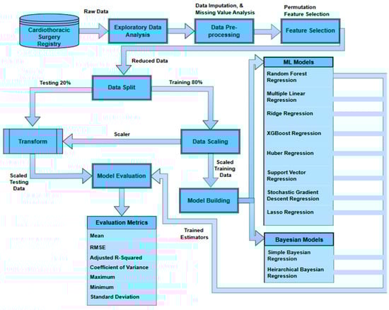
Figure 1.
Overview of the methodology.
3.1. Data Characteristics
Table 1a,b shows an overview of a few dataset variables along with their percentage of missing values (Appendix A: Table A1 contains a complete list of dataset variables, their descriptions, their characteristics, and the percentage of missing values). Among the 68 variables, 12 are continuous with varying distributions (Figure 2), while 52 are categorical variables. The remaining variables are datetime (3) and an identifier (1) for each distinct patient.

Table 1.
(a) Dataset (continuous variables). (b) Dataset (categorical variables).
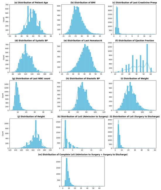
Figure 2.
Distribution of continuous variables.
The dataset contains two variables that impart information about patients’ stay at THI before and after CABG: admission_to_surgey (number of days it takes per patient to go into CABG surgery once admitted) and LOS_surgery_to_discharge (number of days it takes per patient to be discharged after the surgery—recovery period). The overall LoS of a cardiac patient at THI is then the sum of these two variables. The distribution of the overall LoS of patients at THI is shown in Figure 2m. As seen from the graph, the distribution of the LoS is skewed, with the highest frequency at 6 (days) and an average LoS of around 8 (days). The distribution of LoS shows high variability (sd—3.6), with some large values of LoS (>20 days) present at the extreme.
The variable of age is divided into equal ranges (of 10 years) to analyze the trend of patient admissions with age. Figure 3a shows a sharp drop in patients after 70 years, which signifies a low proportion of patients being admitted for CABG procedures with an age greater than or equal to 70 years. This phenomenon can be attributed to multiple factors. Firstly, the incidence of mortality due to cardiovascular diseases is higher in elderly patients as compared to non-elderly patients [32,33]. This should ideally result in a higher influx of patients with an age greater than 70 being admitted for a treatment procedure. However, treating elderly patients for the adverse effects of cardiovascular diseases poses perioperative complications, due to which healthcare professionals treat the symptoms rather than the disease’s cause.
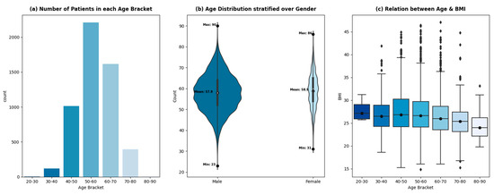
Figure 3.
Relationship between age, gender, and BMI.
With the advent of new, sophisticated procedures, the overall incidence of complications in elderly patients has steadily declined [34]. However, it will take time for it to reflect in the data due to the slow relative adoption in developing countries. The other factor contributing to the low population of elderly patients admitted at THI for CABG is the low life expectancy in Pakistan (65 years) [35].
The ages of the patients being admitted for CABG procedures at THI from 2015–2020 are distributed normally, with an average age of 58 years. The age distribution of the patients stratified by gender is shown in Figure 3b. The female age distribution shows regular spikes at 50, 55, and 60 years, whereas the age distribution of male patients shows a smoother trend. The average age of male and female patients remains comparable (57.9 and 58.9, respectively). The relative width of the plots shows the gender disparity within the dataset. Around 18% of the patients admitted for CABG are female, while 82% are male. A total of 63% of the patients are classified as overweight with a BMI greater than 25 kg/m2, which increases the risk of cardiovascular diseases, according to [36,37]. The prevalence of being overweight exists across all age brackets, however, with different proportions—Figure 3c.
Further analysis of the cohort uncovered a few insights shown in the graphs in Figure 4.
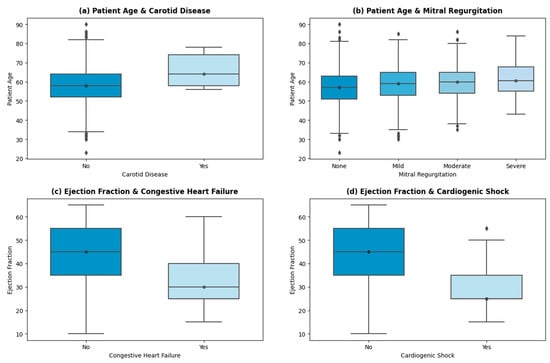
Figure 4.
Important insights.
A linear trend is shown (in Figure 4a) between the patient’s age and the incidence of carotid artery disease (CD). The average age of patients suffering from CD is 66 years, while the average age of patients with no indication of CD is 58 years. Advancing age results in arterial stiffness, structural deformation, and other age-inducing functional alterations, which correlate with a higher risk of carotid disease [38,39,40]. Similar trends are persistent in other high-risk factors, such as arrhythmia and cardiogenic shock. THI uses echocardiography as the primary test for mitral insufficiency/regurgitation. The stratification of the patients into None, Mild, Moderate, and Severe categories is then based on American Society of Echo (ASE) guidelines [41]. Severe mitral regurgitation (MR) is seen in patients with higher ages (with an average age of 61 years). The age of patients with mild to moderate levels of MR is 59 years on average, while patients with no signs of MR have an average age of 56 years. Other valvular regurgitation diseases (aortic and tricuspid) also showed a positive linear trend with age, which is endorsed by ref. [42].
The incidence of congestive heart failure (HF) is higher in patients with a mean left valve ejection fraction (EF) of 32%. A total of 329 patients showed HF with reduced EF (less than 40%), 75 showed HF with mid-range EF (between 40% and 49%), and 52 encountered HF with preserved EF (levels greater than 50%). The patient stratification of HF at THI concerning EF levels is based on US guidelines [43,44]. As per Figure 4d, patients with cardiogenic shock presentation on admission have a mean EF of 29.6%. Cardiogenic shock is caused by decreased contractility or decreased filling of the heart, mostly the former. The low contractility causes low cardiac output and depressed ventricular systolic function, which is persistent in patients with reduced HF [45].
3.1.1. Data Cleaning and Imputation
The analysis and audit of the data showed a very minimal amount of missing data (≈2.53% cumulative). The variable BPsystolic shows the highest missing rate of 0.48%, followed by diastolic, pulmonary_artery_done, last_wbc_count, BMI, and pulmonary_insufficiency with identical missing rates of 0.41%.
The variables were imputed with other variables as a reference. For example, the data for BMI was filled with calculated BMI using weight and height parameters. Similarly, the variable BPsystolic was imputed by the dichotomous variable of hypertension. The values of BPsystolic were averaged against patients whose hypertension label was ‘Yes’ (mean—124 mmHg). Similarly, for patients with hypertension labeled ‘No’, a different mean of BPsystolic was acquired (mean—117 mmHg). These two mean values were then used to fill in the missing values of the variable BPsystolic, with hypertension as a reference. A similar strategy was used to impute values for the diastolic variable as well. The observations with missing values for pulmonary_artey_done, last_wbc_count, and pulmonary_insufficiency attributes account for 1.3% of all the missing values. The cumulative missing rate for these variables is less than the benchmark of 5% and hence can be safely removed [46] without any adverse effects on the model predictions.
3.1.2. Data Preparation
The variable TempSNO is removed from the model-building process as it is an identifier for a patient and does not contribute to the estimation. Similarly, all datetime variables (date_of_discharge, date_of_admission, and date_of_surgery) were also removed from the dataset as the information imparted from these variables is already encoded in the variables Admission_to_surgery (days) and LOS_Surgery_to_discharge (days). The variables weight and height were subsequently removed after calculating and filling in the BMI variable.
To estimate the overall LoS of a cardiac patient at THI, the variables Admission_to_surgery and LOS_Surgery_to_discharge are added together to create a new target variable, LOS. Consequently, these variables are removed from the dataset after creating the new target variable. The resulting dataset has 61 features (including the newly created target variable LoS).
All the categorical variables are label encoded (starting with 0), and the continuous variables are scaled between 0 and 1 (Min–Max scaling). Min–Max scaling retains the natural order (distance) between the data points while reducing the effect of their magnitude on the target variable. Without this normalization, variables with large values can result in biased estimates. The normalization step is performed after splitting the dataset into training and testing sets. The scaler is fitted to the training data and then used to transform both the training and testing datasets to minimize data leakage. The scaling parameters learned on the training set are used to transform the testing set as well, because scaling parameters for testing data are not known in real life. Hence, using the scaling parameters of the testing set for the scaling of testing data would make the model aware of the distribution of the testing set, introducing leakage and overestimated accuracy.
3.2. Permutation Feature Importance (PFI)
PFI evaluates the increase in the models’ score when a feature effect is removed. The change in model accuracy before and after the removal of the variable gives an insight into the relative importance of a feature [47]. PFI is used due to its robustness against overfitting. If the dataset contains uncorrelated variables, then a feature selection method can increase the effect of a feature that is not predictive of the outcome [48]. The PFI method solves this issue by testing the variable’s importance in terms of model accuracy. It ensures that only those features are included in the sample space that contribute positively to the accuracy of the model. In addition to gauging the variable’s importance, PFI helps to gauge the feature interactions and their contribution to the loss as well. It perturbs the feature of interest, effectively removing its interaction with other variables. The relative change in the model performance is then indicative of main and interaction feature effects. Impurity-based feature selection methods (decision trees and random forests) show a bias towards high cardinal and numerical variables as they show greater affinity towards the scale of measurement of a variable [49]. The dataset of this study contains numerical variables with different magnitudes and categorical variables with high cardinality, which results in under- or overestimated variable influence using impurity-based feature selection methods. Greedy algorithms for feature selection, such as recursive feature elimination (RFE) and sequential feature selection (SFS), are good at removing redundant variables from a dataset, resulting in an optimum number of features defined a priori. These methods recursively add or remove a feature from the dataset, retrain the model, and gauge the changes in model performance, which makes them undesirable for datasets with a large number of variables due to increased runtimes. Furthermore, defining a suitable number of reduced parameter spaces a priori is suboptimal for the overall performance of the model. Defining a low number of features would result in an underperforming model, and a large number would result in high time complexity. This study aims to predict the LoS for cardiac patients where a tradeoff on accuracy is not desirable. Hence, PFI is used as a feature selection method to ensure the presence of only those variables that positively contribute to the accuracy of the model.
PFI requires a trained model (on all features) with known accuracy. The variables are then removed recursively to assess the change in accuracy. This research uses a random forest regressor (trained on 60 independent variables) as the base model to assess feature importance.
To assess the effect of a variable on the model’s overall performance, the effect of column must be removed and replaced by a vector of the same dimension. This new vector, or augmented feature vector, is sampled from the same distribution as the feature of interest. This ensures a break between the target and the feature, hence simulating the effect of the absence of the feature. The model is tested on augmented data (with the permutated feature), and the new score is determined. The change in the score translates into the importance of the said feature.
Let be a feature of the dataset D such that each belongs to the feature set , where . If the output of the model trained on dataset D is , then the output of the model on augmented dataset (dataset with permutated column) is the average accuracy over permutations of feature , given as . The change in accuracy or permutation feature importance of is then given by:
The training dataset is divided into two further sets of training and testing samples. A total of 80% of the training data are used to train a Random Forest regressor with the complete feature set (60 variables). The remaining 20% of the training data are then used to recursively test the model’s performance when a feature effect is removed. One way to remove the feature effect is to remove that feature from the feature set entirely. However, as the baseline model is trained on all independent variables (60 variables), the model expects 60 variables for testing as well. Hence, removing a feature would result in an error while testing the model’s performance. That is why a vector of the same dimension (as the feature to be removed) is sampled from the same distribution as that of the variable of interest. For instance, to measure the importance of last_cretenine_preop in predicting the LoS, the variable is replaced with the randomized version of the same feature in the test set. This randomization removes any information or effect that last_cretenine_preop may have on the target variable. The model is then tested on the validation set, and the resultant RMSE is compared to the RMSE with all the features. Any increase or decrease in the resultant RMSE will dictate the effect of last_cretenine_preop on the LoS.
Table 2 shows the features selected by the permutation feature selection method with a decreasing order of change to the accuracy of the model.
Table 2.
List of features from the permutation feature importance method.
3.3. Models
3.3.1. Simple Bayesian Regression Model (SBM)
To model the problem of LoS prediction in the Bayesian paradigm, it is imperative that an empirical relationship be identified that links the target variable with its parameters. Consider the following relationship:
The above equation is similar to an accelerated failure time (AFT) model proposed by ref. [50], which is used to predict the occurrence of an event in time T. If the event in the AFT model is taken as the influx of patients, then the time T can be thought of as the expected length of stay for a patient. Rewriting the above equation tailored to the LoS problem gives:
Β′ is a vector of coefficients of dimension n, where n = 44 is the number of features determined by the permutation feature selection method. Each β is sampled from a prior distribution. A prior distribution is knowledge about the dataset’s variables before any evidence is considered. It can be any probability distribution based on domain knowledge and variable characteristics. X′ is the training data of dimensions m × n, where n is the reduced feature space, m is the number of training samples (80% of the data), and β0 is the intercept.
Given the target variable’s continuous and numerically positive nature, posterior sampling must be conducted from an always positive continuous probability distribution. A truncated normal distribution is used as the likelihood for SBM. The truncation is performed to keep the values continuous and positive. The priors for the model can be initiated with weakly informative priors [51]. The model specifications for SBM are then:
where , , , and are the hyperpriors and are sampled from normal and half-normal distributions, respectively.
For a simple Bayesian regression model (SBM), the equation for likelihood is:
The Markov Chain Monte Carlo (MCMC) simulation method [52] is used to estimate the posterior resulting from the above priors and the likelihood function. The MCMC method iteratively samples values from the posterior until convergence or equilibrium is reached (the transition probability reaches the stationary probability distribution). The parameters that result in the said convergence are the estimated parameters of the model. The sampling process is governed by a sampling algorithm such as the Metropolis algorithm [53], Gibbs sampler [54], and No-U-Turn Sampler (NUTS) [55].
To approximate the posterior distribution resulting from the above-mentioned model specification, the study uses the implementation of a No-U-Turn Sampler (NUTS) from the PyMC package [56].
3.3.2. Hierarchical Bayesian Regression Model
This study evaluates hierarchical Bayesian regression in addition to simple Bayesian regression, as it is more robust to the variability of the data. Most of the values of LoS are concentrated between the ranges of 0–10, with some values spread far apart. Building a non-hierarchical Bayesian regression model would then result in a bias towards values with a high frequency and would not be able to predict tail values. One way to improve model performance is to divide the dataset into smaller parts such that each subset is locally similar with low variability. Smaller models are trained on each subset of the data. The combination of these smaller models is known as an un-pooled model and can result in better accuracy. However, this kind of model is prone to overfitting due to small subsets of the data. All the models are independent of each other, with no knowledge transfer in between. Latent information is lost and results in deficient performance on test sets. On the contrary, multilevel, hierarchical, or partially pooled models allow knowledge sharing between sub-models, which helps them capture the variability of the target variable.
To use the method of hierarchical Bayesian regression, the target variable of LoS is divided into four distinct ranges of values (Figure 5).

Figure 5.
Levels of LoS.
The four LoS levels do not mean that the dataset is divided into subsets (as in an un-pooled model); instead, it is indexed to let the model know that it must learn different posterior distributions for these levels of LoS yet maintain the optimum flow of knowledge between the distributions to capture the variability in the best possible way.
The records of patients with an LoS between 0–10 are indexed with 0, the LoS between 10–20 are indexed with 1, the LoS between 20–30 are indexed with 2, and the LoS greater than 30 are indexed with 3. This indexing of the dataset based on the LoS ranges acts as ‘levels’ for Bayesian regression. The priors are initialized differently for each ‘level’ in the dataset. Instead of sampling 44 priors for β′, 1 for β0, and 1 for (in a typical Bayesian regression model), the hierarchical model will sample 44 × 4 priors for β′, 4 for β0, and 1 for , corresponding to each level in the dataset. Hence, modify the regression equation as follows:
where level is a hierarchical variable guiding the sampling of the Bayesian model. This variable is not used in the training or testing of the model. It is used to tell the Bayesian sampler to change the sampling space as the level is changed.
The Bayesian model would then sample different priors with different distribution parameters to learn the posterior for each level. The sampler would run until the model could estimate the best distribution for each level of the LoS, hence capturing the heterogeneity of the target variable. The model specification for HBM is almost similar to that for SBM, with an added sampling layer for each level. Since the estimation equation has an index, ‘level’, for sampling different distributions for each hierarchy, the likelihood form for HBM is adopted to incorporate this effect:
The coefficients and errors are sampled from normal distributions.
where , , , and are the hyperpriors and are sampled from normal and half-normal distributions, respectively.
The learning process is similar to that of SBM. The PyMC package is used to create and train the model with NUTS as a sampler algorithm.
3.3.3. ML Models
The following Table 3 shows the ML models used in this study for LoS prediction.
Table 3.
ML models.
The implementation of the ML models used in the study is performed using the sklearn library [63] of the Python programming language.
The code used in the study for the creation and testing of the models is available at Github [64].
4. Results
The hierarchical Bayesian inference with MCMC on features selected by permutation feature selection resulted in the lowest root mean square error (RMSE) and mean absolute error (MAE) of 1.49 and 1.16, respectively, which is a considerable improvement over the values achieved by ML methods. Table 4 shows the results of the models on testing data benchmarked against various evaluation metrics.
Table 4.
Statistical summary of the target variable—actual and estimated.
The table shows that all models except SVR were able to estimate the mean of the testing sample with acceptable precision. However, significant differences arise when other statistical measures are analyzed. Only HBM managed to capture the spread of the actual testing data (as seen from the standard deviation values). All the other models failed to capture the variability of the data accurately. The prevalence of extreme values in the data made it difficult for ML models to accurately predict large or exceedingly small values. By analyzing the standard deviations of the predicted values, it is evident that almost no variability in the actual data was estimated by the ML models. ML models under-predicted the standard deviation of the testing sample, which means they could only identify the most frequent values and could not estimate seldom occurring extreme values. A similar phenomenon can be seen by observing each model’s minimum and maximum predicted values (rounded to the nearest whole number).
The coefficient of variance (CV) is a statistical measure of the dispersion of values around the mean. The LoS variable has a CV of 0.43, meaning that most of the values are packed around the mean, with some extreme values in between. If the variable LoS had been completely homogenous, then the coefficient of variance would have been less than 0.20 [65]. The CV for all models is relatively small (smaller than 0.21), which shows that almost all the predicted values (from all ML models along with simple Bayesian regression as well) are present around the mean of the sample while ignoring the presence of extreme values.
Furthermore, the adjusted R-squared for HBM is drastically better than the other models. The exceptionally low adjusted R-squared value for all ML models translates into their inability to capture the variance of the target variable. Lasso shows a negative adjusted R-squared, which means the model could not predict the mean value for most of the testing samples, showing a poor fit.
One interesting trend can be observed by analyzing the RMSE values for the models. All the ML models (except LR) had comparable RMSE (3.2–3.3). Even with hyperparameter tuning, the RMSE did not change, which shows that all these models were ‘stuck’ at the local minima. No performance gains were observed beyond the RMSE of 3.23. Given that most of the values of the target variable lay in the range of 5–8, all the models ended up generating biased predictions around this range. Even Bayesian inference did not show any improvement in the RMSE until the model was changed into a hierarchical regression model (RMSE—1.49).
Figure 6 shows the Taylor diagram [66] comparing ML and Bayesian model performances with the testing data. The HBM model showed better results in all three statistics (correlation—0.913, given by the azimuth angle; standard deviation—3.2, given by blue dotted contours; and centered root mean square—1.49, given by green contours). All other models showed relatively lower and similar performance in simulating the observed testing data. These models ended up capturing only the mode of the actual data distribution while underperforming on extreme data points. This adversely affected the ML and SBM model estimates, resulting in their lower performance across all evaluation metrics.
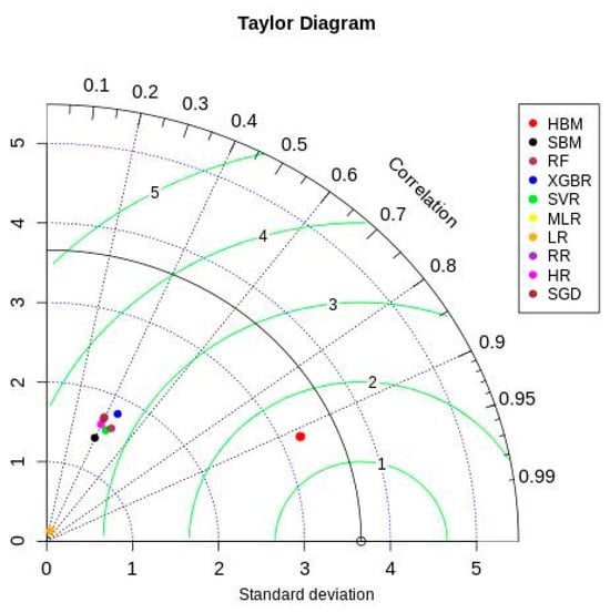
Figure 6.
Taylor diagram.
Bayesian inference uses a sampler to sample values from specified priors and likelihood to estimate the posterior distribution of the model. The sampling process is crucial for Bayesian models to approximate the parameters. To check the adequacy of the sampling process, a trace plot of the posteriors of the variables is used. Figure 7 and Figure 8 show trace plots of SBM and HBM, respectively.

Figure 7.
SBM trace plot showing the sampling of (Markov) chains using a NUTS sampler.
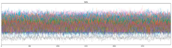
Figure 8.
HBM trace plot showing the sampling of (Markov) chains using a NUTS sampler.
The sampling process (using a NUTS sampler) uses 4 chains, each with 3000 samples and 1000 tuning steps. Each colored line in Figure 7 and Figure 8 represents the sampling path of a chain. At each step, the NUTS sampler chooses a value for each parameter from their respective priors and accepts or rejects the sampled values based on acceptance probabilities (implemented natively by the NUTS sampler). Consequent sampling of values at each step, along with their acceptance or rejection, creates a sampling path. Figure 8 shows the random snake-like movement of the chains, which underlines effective exploration of the parameter space defined by the model priors and hyper-priors. It is important that the chains wander around the parameter space in an ergodic manner to ensure convergence. The significant overlap and mixing of the chains in Figure 8 (hairy caterpillar structure) [67] reflects good convergence, which translates into a proper model configuration. Furthermore, the absence of strong trends or jumps in the trace plot of HBM suggests that the MCMC algorithm is efficiently traversing the parameter space, ensuring a more thorough and unbiased exploration.
However, as seen from the trace plot of SBM, the (Markov) chains show irregular sampling with persistent divergences, signifying that the posterior of the parameters varies significantly. In other words, the sampling process did not manage to converge on the correct posteriors for the model parameters, resulting in varying estimations across the chain. The sampling chains in the SBM plot show considerably less mixing and overlap (as compared to the HBM trace plot), along with a few chains showing large jumps with no exploration of the parameter space. This can be attributed to the high variability and skewness of the data. The divergence of the sampling chains warrants model improvements and usually vanishes when a more comprehensive model is specified. This can be seen from the trace plot of HBM having no divergences, signifying the correct model specification.
Another convergence diagnostic is the Gelman Rubin () score [68] (for each parameter), which assesses the variation in the sampled values at the start of the sampling process against the sampled values at the end. The closer the values are to 1, the better the model’s convergence. The score for parameters estimated using SBM showed deviations from the optimum value, signifying that the sampling process did not converge to a stationary distribution, unlike the score for parameters estimated using HBM (given in Appendix B).
5. Discussion
The results of this study’s experiments showed that the HBM model outperformed its simpler variant along with other ML models for LoS prediction of cardiac patients undergoing CABG surgery based on their pre-operative variables. Hence, the subsequent part of the discussion explains the estimated coefficients of HBM only (parameter coefficients for other models are given in Appendix C (Table A8, Table A9, Table A10, Table A11, Table A12, Table A13 and Table A14)).
Bayesian estimates of the parameters identified the critical biomarkers affecting the LoS. According to the magnitude and the sign associated with each coefficient value, varying degrees of effects on the target variable can be identified. The HBM estimated four sets of coefficient posteriors for each level of the target variable. Bayesian models output learned distributions of the parameters of the model instead of point estimates. This is useful when greater interpretability of the model is required in terms of causality and uncertainty. The Bayesian models quantify the model’s uncertainty in terms of the deviation/spread of the values in the posterior distributions of the parameters. Table 5a–d shows interval mean values of the estimated parameters.
Table 5.
(a) Estimated parameter coefficient value (level 0). (b) Estimated parameter coefficient value (level 1). (c) Estimated parameter coefficient value (level 2). (d) Estimated parameter coefficient value (level 3).
The four different sets of coefficient values corresponding to different ranges of the LoS variable are useful to identify the varying effects a similar predictor might have on the LoS of a patient. The results of the HBM show that when the LoS of a patient changes from one level to another, the factors contributing to their LoS also change. These changes can be tracked in terms of parameter importance, quantified as the mean of the posterior. These parameter changes conditioned on LoS levels can enable a clinician to assess which factors play a crucial role in determining the lower or higher LoS of a patient, hence offering better explainability than a typical regression model.
Table 5a shows high linearity between a patient’s age and level 0 LoS (between 0–10 days), as cardiac complications are more prevalent in older patients. As age increases, the LoS of a patient also increases. In addition to patient age, arrhythmia, usage of nitrates IV, and pre-operative creatinine levels are the most impactful predictors for level 1 LoS (between 0–10 days) [69]. By analyzing Table 5b of level 1 LoS (between 10–20 days), it is evident that age is still a prominent factor in increasing LoS in cardiac patients. However, the effect of age is not profound, which tells a clinician that there are other factors apart from age that might cause the LoS to increase. MI_timing (time between myocardial infraction and CABG procedure), use of ace inhibitors, family history of cardiovascular disease, diastolic BP, pulmonary artery hypertension, NYHA_class, and PCI_timing (time between incidence of angioplasty and current time) are more prominent factors explaining the LoS between 10–20 days. A total of 44% of patients with LoS between 10–20 days underwent CABG procedures within 1–7 days of the incidence of myocardial infraction, signifying a greater need for patient stabilization before invasive procedures, as compared to only 24% of patients with LoS level 0 (between 0–10) needing additional prep and stabilization times. Similarly, 47% of the patients with LoS level 1 had a higher NYHA risk category as compared to only 29.5% of patients with LoS level 0. In other words, the effect of critical features is more profound at higher LoS levels as compared to lower levels [19].
LoS levels 1 and 2 share quite a few parameters; however, they differ in their magnitudes. The difference in magnitudes suggests that the variable itself takes on larger values and results in a higher contribution towards increasing LoS beyond 20 days. Arrhythmia is a prominent factor in determining the LoS between 0 and 20 days (level 0 and level 1), as seen in Table 5a,b. However, as LoS increases beyond level 1, there are other ‘derived’ factors that become more important; irregular diastolic pressure due to arrhythmia becomes more prevalent in patients with LoS between 20 and 30 days, or abnormal breathing signifies a higher New York Heart Association class of heart failure resulting in level 3 LoS. Additionally, the days required to stabilize and prep the patient before CABG are significantly increased due to the high-risk nature of the patient, coupled with any cardiac complications at the time of admission, resulting in a prolonged LoS (level 3) [70].
Parameter estimation with HBM showed an interesting insight involving the inverse relation between high-risk variables and the LoS. Levels 0 and 1 LoS tend to decrease in the presence of cardiogenic shock. The relationship seems counterintuitive given the high-risk nature of the parameter. However, a deeper analysis of the population showed that patients with a history of cardiogenic shock (or experiencing one just after admission) tend to pass away due to complications, resulting in a shorter stay. Hence, it is clinically relevant. These inverse relationships of high-risk variables with the LoS impart significant information about the mortality risk associated with an inpatient. With these relationships, a new high-risk stratification method can be developed. Clinically relevant variables with a high linear or inverse relationship with LoS can be used to classify the morbidity of cardiac patients, where high-risk patients could be subjected to more extreme medical protocols at an early stage, which can help increase survival chances.
The study compares and evaluates the predictive efficacy of various frequentist and Bayesian regression models to aid and encourage healthcare professionals and researchers to explore the Bayesian paradigm of modeling, especially for LoS, which is highly heterogonous and positively skewed. Most of the literature on LoS prediction uses machine learning models and caters to the variability in the target variable by either removing the outliers or capping the values at a maximum [17]. Another method employed by the researchers is to convert the continuous variable LoS to a dichotomous (early/prolonged) or a categorical variable with multiple bins and ranges (Table 6). This methodology transforms the nature of the problem from a regression to a classification. However, this study treats the LoS as a continuous variable without removing extreme tail values to homogenize the data. The hierarchical Bayesian model of this study outperforms other models from the literature that use ML regression models, with the exception of ref. [15], which reports a low MSE of 0.68 with artificial neural networks. However, the range of the target variable used in the study is short and homogenous: 1–8 days. Whereas, the LoS used in this study ranges from 1 to 65 with high variability.
Table 6.
Comparing studies from the literature where the objective is LoS prediction and at least a single learning model and its findings are reported.
This study uses only pre-operative clinical features to model the LoS of cardiac patients undergoing CABG. Early identification of LoS is more valuable for healthcare institutions than later predictions. Multiple studies explore LoS prediction based on early indicators with varying degrees of accuracy. However, this study shows the best performance among all others when HBM is used for predictions on the skewed distribution of the target variable.
Very few studies in the literature model the LoS in the Bayesian paradigm. Most notable among these are the studies by Suez-Castillo et al. [29] and Ng et al. [30]. Suez-Castillo et al. propose an asymmetric link function to stratify the incidence of nosomial infection in patients (at North Area Hospital, Jaen, Spain) and its effect on the patient’s length of stay. The researchers compared Bayesian and frequentist estimation of symmetric and asymmetric logistic link function parameters and report an improvement in AUC score with Bayesian estimation of symmetric (AUC—0.96) and asymmetric (AUC—0.99) logit models. The authors extended the study to model the LoS of patients using the Poisson-Gamma model in Bayesian and frequentist paradigms. The authors used non-informative normal priors (similar to this study) for the covariates with the additional novel parameter to model the randomness (increase or decrease in LoS) resulting from the incidence of nosomial infection after admission. The study used the MCMC method for parameter estimation (similar to this study) and reported sound convergence of the sampling chains. Ng et al. modeled LoS using linear mixture models to accommodate for random effects introduced by the heterogeneity of the target variable and the cohort. The authors used the data of neonates from 23 hospitals across Western Australia from 1998–1999 and modeled the short- and long-term LoS to identify the risk factors. The study used the expectation maximization strategy instead of the MCMC method for the estimation of coefficients and reported impressively lower standard errors. The authors show that prolonged LoS is primarily due to derived factors originating from the sudden complications and severity of the other covariates, which is concordant to the results of this study. Major differences exist in the objective of the study as well as the cohort. This study uses only pre-operative variables for the LoS prediction of cardiac patients; however, both the studies described above used pre- and intra-operative variables as well. Furthermore, the objective of these studies is to model the LoS in terms of its covariates to assess and identify the high-risk factors. Both studies managed to model the data-generating process and report coefficient estimates that closely resembled the original data. However, these studies did not provide out-of-sample predictions of LoS using the learned model coefficients. Furthermore, among all studies, only Suez-Castillo et al. provided a comparative analysis of the results of Bayesian and frequentist models; however, the frequentist methods used are limited and non-trivial (Poisson-Gamma regression model), with no comparison of predictive prowess.
Local studies that predict LoS include Siddiqa et al. [71] and Bajwa et al. [72]. Among these, ref. [72] is a more specialized study carried out in a tertiary care burn center in Lahore, Pakistan. The authors categorized the target variable of LoS into classes and used logistic regression for prediction with an AUC of 0.96. The study uses pre-operative variables for prediction, similar to this study; however, the experiments are limited to ML and other survival models only. Siddiqa et al. used MLR, lasso, ridge, DT, XGB, and RF regression models for LoS prediction on pre- and intra-operative data of patients from the healthdata.gov database. The study reports the RF regression model as the best performing one, with an RMSE of 2.23 (MSE—5) as compared to the RMSE of 1.49 achieved in this study using only pre-operative variables modeled using hierarchical Bayesian regression.
6. Limitations
The study aims to model the LoS of cardiac patients undergoing CABG surgery while evaluating frequentist and Bayesian regression models to aid and facilitate the healthcare community in exploring the Bayesian paradigm for the LoS problem. The study is carried out on a dataset of one healthcare institution. The study is limited in terms of its cohort. It might be useful to consider the data from multiple health care centers to gauge the changes in predictive accuracy of Bayesian and frequentist methods in the presence of increased data size. Bayesian models generalize better to the target population; however, they have high complexity in terms of their design and execution times. The training time increases with the addition of more data; hence, a tradeoff between runtime and accuracy is usually needed.
Moreover, the study uses only pre-operative variables for early LoS prediction, which is more desirable as earlier estimates of a patient’s stay help institutes with timely resource and personnel allocation. However, this limits the accuracy of the model predictions as more definitive and critical factors are mostly available peri- or post-operatively. This tradeoff between earlier versus accurate predictions can be solved by using a dynamic model, which can update its predictions with the advent of new data. This would lead to better visibility of the patient’s hospital stay through various stages of hospitalization. Hierarchical Bayesian regression offers interpretability in terms of changing coefficient values across different levels/hierarchies. By analyzing the changes in magnitude and direction (sign) of a variable across various hierarchies, useful insights can be obtained.
Future work can be conducted to explore the use of the Shapley Additive Explanations (SHAP) paradigm of interpretation in Bayesian models. SHAP is not directly applicable to Bayesian models (especially hierarchical models) because they produce posterior distributions for the coefficients instead of point estimates. Hence, calculating SHAP values for each sample in the posterior distribution would be computationally expensive. However, research in the area of integrating open source Bayesian modeling libraries (PyMC and Stan) to support SHAP natively is an interesting and profound area of interest, with applications extending to the healthcare domain.
7. Conclusions
Hierarchical variants of Bayesian inference with MCMC methods have proven to be useful for predicting LoS in cardiac patients based on their pre-operative variables. The accuracy shown by the hierarchical Bayesian regression model is better (RMSE—1.49, MAE—1.16) than that of ML models when data variability is high with extreme values, with the added advantage of greater interpretability. From the results of this study, it is evident that a simple Bayesian regression model without hierarchy is insufficient to explain the variability of the data.
Furthermore, many ML models also fell short of capturing the real variance of the dataset, especially when the data are highly volatile. The HBM is especially useful when the target variable has different value ranges. ‘Soft’ division of the dataset into groups or levels (by indexing) can be used to create a hierarchy of heterogeneous, continuous variables. A separate set of parameter values for each level in the LoS variable helps assess the effect of clinical variables as LoS increases in a patient. Analyzing the varying effects of the same variable across different LoS ranges will help the clinician plan the appropriate intervention.
By using Bayesian inference quantification (with hierarchical changes) of the parameter, medical staff can create a mechanism of risk stratification where the high-risk features affecting the LoS the most (linearly or inversely) can be known beforehand. This will enable clinicians and administrative staff to look for these factors in an in-patient, classify them as high-risk, and release resources accordingly. Bayesian inference methods (especially hierarchical Bayesian models) are computationally extensive but result in good estimates with better clinical explainability.
Author Contributions
Conceptualization, T.M., I.A. (Ibrahim Abdurrab), S.A. and S.S.; Methodology, I.A. (Ibrahim Abdurrab), T.M. and A.B.A.; Software, I.A. (Ibrahim Abdurrab); Formal Analysis, T.M., S.S., G.P. and S.A.; Data Curation, M.K. and I.A. (Imran Ali); Validation, A.P., A.M., S.S., S.A., G.P. and M.K.; Writing—Original Draft, I.A. (Ibrahim Abdurrab) and T.M.; Writing—Review and Editing, I.A. (Ibrahim Abdurrab), T.M., M.S.S. and A.B.A.; Supervision, T.M. and M.S.S. All authors have read and agreed to the published version of the manuscript.
Funding
This research received no external funding.
Institutional Review Board Statement
Not applicable.
Informed Consent Statement
Not applicable.
Data Availability Statement
Data are contained within the article.
Acknowledgments
The authors extend their gratitude towards the team at Tabba Heart Institute for providing the data of their patients along with their time to discuss, assess, and validate the results of the study. Also, the authors recognize the contributions of the Institute of Business Administration, Karachi, in providing the necessary resources and access to their Big Data Lab for running and validating the experiments.
Conflicts of Interest
The authors declare no conflict of interest.
Appendix A. Dataset Overview
Table A1.
Variable description (Continuous).
Table A1.
Variable description (Continuous).
| Feature | Description | Type | Min | Max | Average | Std | IQR | % of Missing Values |
|---|---|---|---|---|---|---|---|---|
| TempSNO | Serial number | Incremental | ||||||
| date_of_admission | Admission date | datetime | 25 November 2015 | 30 December 2020 | 0 | |||
| date_of_surgery | Surgery date | datetime | 28 November 2015 | 31 December 2020 | 0 | |||
| date_of_discharge | Discharge date | datetime | 5 December 2015 | 7 January 2021 | 0 | |||
| patient_age | Age of patient (Years) | Continuous | 23 | 90 | 58.07 | 8.66 | 12 | 0 |
| Admission_to_surgery | Admission to surgery (Days) | Continuous | 0 | 21 | 2.26 | 1.94 | 2 | 0 |
| LOS_Surgery_to_discharge | Surgery to discharge (Days) | Continuous | 0 | 59 | 6.04 | 2.97 | 1 | 0 |
| last_wbc_count | Last WBC count (×109/L) | Continuous | 2.8 | 48.8 | 9.48 | 2.77 | 3.1 | 0.41 |
| BMI | BMI (kg/m2) | Continuous | 14.82 | 47.08 | 26.82 | 4.35 | 5.47 | 0.41 |
| last_hematocrit | Last hematocrit value (%) | Continuous | 21.2 | 56.2 | 40.51 | 4.92 | 6.6 | 0 |
| last_cretenine_preop | Last creatinine value (mg/dL) | Continuous | 0.41 | 13.3 | 1.14 | 0.63 | 0.32 | 0 |
| BPsystolic | Pre-operative systolic BP (mmHg) | Continuous | 76 | 199 | 122.49 | 15.94 | 23 | 0.48 |
| diastolic | Pre-operative diastolic BP (mmHg) | Continuous | 27 | 117 | 70.36 | 9.63 | 14 | 0.41 |
| ejection_fraction | Pre-operative LV ejection fraction (%) | Continuous | 10 | 65 | 42.89 | 11.18 | 20 | 0 |
| Weight | Weight of the patient (kg) | Continuous | 36 | 128 | 71.87 | 12.74 | 17 | 0 |
| Height | Height of the patient (cm) | Continuous | 123 | 191 | 163.6 | 8.33 | 10 | 0 |
Table A2.
Variable description (Categorical).
Table A2.
Variable description (Categorical).
| Feature | Description | Type | Labels | n (%) | % of Missing Values |
|---|---|---|---|---|---|
| gender_id | Gender of patient | Categorical | Male, Female | 4360 (82), 954 (17.9) | |
| pulmonary_artery_done | Test for pulmonary artery mean pressure conducted? | Categorical | Yes, No | 2205 (41.4), 3109 (58.5) | 0.41 |
| Active_tobacco_use | Tobacco use within last 6 months | Categorical | Yes, No | 1308 (25.8), 3975 (74.1) | |
| f_history_cad | Family history of coronary artery disease | Categorical | Yes, No | 2664 (49.6), 2699 (50.3) | |
| diabetes | Diabetes/insulin use | Categorical | 2067 (38.5), 2211 (41.2), 1085 (20.3) | ||
| myocardial_infarction | Any prior myocardial infarction (MI) | Categorical | Yes, No | 3816 (71.1), 1547 (28.8) | |
| MI_timing | Time between MI and CABG | Categorical | 1584 (29.5), 16 (0.29), 26 (0.48), 1473 (27.4), 938 (17.4), 1326 (24.7) | ||
| congestive_heart_failure_A | Congestive heart failure | Categorical | Yes, No | 471 (8.7), 4892 (91.2) | |
| NYHA_class | NYHA (New York Heart Association shortness of breath class) during last 2 weeks | Categorical | 2482 (46.2), 62 (1.1), 1059 (19.7), 1513 (28.2), 247 (4.6) | ||
| Cardiac_Presentation_on_Admission | Cardiac symptoms on arrival | Categorical | 301 (5.6), 370 (6.8), 575 (10.7), 1664 (31.0), 1778 (33.1), 675 (12.5) | ||
| Angina_class | Angina Canadian Cardiac Society (CCS) classification within last 2 weeks | Categorical | 1069 (19.7), 26 (0.48), 700 (13.0), 2443 (45.5), 1135 (21.1) | ||
| cardiogenic_shock | Cardiogenic shock at the time of CABG | Categorical | Yes, No | 65 (1.21), 5298 (98.7) | |
| resuscitation | Any cardiac resuscitation within one hour of CABG | Categorical | Yes, No | 15 (0.27), 5348 (99.7) | |
| arrhythmia | Any prior arrhythmia | Categorical | Yes, No | 122 (2.27), 5241 (97.7) | |
| SustVTVF | Sustained VT/VF within 2 weeks | Categorical | Yes, No | 60 (1.11), 5303 (98.8) | |
| AFibFlutter | Afib/Flutter within 2 weeks | Categorical | None, Afib/Flutter, Heart block | 5298 (98.7), 51 (0.95), 14 (0.26) | |
| ventilator_used | Patient already on ventilator | Categorical | Yes, No | 76 (1.41), 5287 (98.5) | |
| beta_blockers_A | Beta blockers within 24 h | Categorical | Yes, No | 4593 (85.6), 770 (14.3) | |
| ace_inhibitors_A | ACE inhibitors within 24 h | Categorical | Yes, No | 1116 (20.8), 4247 (79.1) | |
| nitratesIV | Nitrates I.V at time of CABG | Categorical | Yes, No | 553 (10.3), 4810 (89.6) | |
| anti_coagulants | Anticoagulants within 48 h prior to surgery | Categorical | No, UFH, LMWH, Thrombin inhibitors | 4061 (75.7), 924 (17.2), 375 (6.9), 3 (0.05) | |
| warfarin_A | Warfarin within 24 h of CABG | Categorical | Yes, No | 5254 (97.9), 109 (2.1) | |
| inotropes | Inotropes within 48 h | Categorical | Yes, No | 76 (1.4), 5287 (98.6) | |
| steroids | Steroids witihn 24 h | Categorical | Yes, No | 5 (0.1), 5358 (99.9) | |
| aspirin_A | Aspirin within 5 days of CABG | Categorical | Yes, No | 4758 (88.7), 605 (11.3) | |
| lipid_lowering_A | Any lipid-lowering medications within 24 h of CABG | Categorical | Yes, No | 4696 (87.6), 667 (12.4) | |
| Dyslipidemia | Dyslipidemia with statins | Categorical | No, Yes (On Statin), Yes (Not on Statin) | 11 (0.2), 3254 (60.7), 2091 (39.0), 7 (0.1) | |
| dialysis | Hemodialysis-dependent pre-operatively | Categorical | Yes, No | 42 (0.8), 5321 (99.2) | |
| hypertension | Hypertension | Categorical | Yes, No | 3859 (72.0), 1504 (28.0) | |
| Cerebovascular_disease | Any cerebrovascular disease | Categorical | Yes, No | 283 (5.3), 5080 (94.7) | |
| pulmonary_insuff | Pulmonic insufficiency | Categorical | None, Trivial, Mild, Moderate, Severe | 4705 (87.7), 438 (8.2), 188 (3.5), 6 (0.1), 4 (0.1) | |
| Carotid_disease | Carotid disease | Categorical | Yes, No | 7 (0.1), 5356 (99.9) | |
| chronic_lung_disease | Chronic lung disease | Categorical | Yes, No | 119 (2.2), 5244 (97.8) | |
| FirstCVSurgery | Incidence of CV surgery | Categorical | First CV Surgery, 2nd CV surgery, 3rd CV surgery, 4th CV surgery | 5341 (99.6), 19 (0.4), 2 (0.0), 1 (0.0) | |
| previous_cv_interventions | Previous CV interventions (prior PCI, CABG, or others) | Categorical | Yes, No | 720 (13.4), 4643 (86.6) | |
| previous_coronary_bypass | Previous coronary bypass (CABG) | Categorical | Yes, No | 21 (0.4), 5342 (99.6) | |
| previous_valve | Previous valve surgery | Categorical | Yes, No | 1 (0.0), 5362 (100.0) | |
| intracardiac_device | Previous intracardiac device pacemaker or defibrillator (PPM or ICD) usage | Categorical | Yes, No | 11 (0.2), 5352 (99.8) | |
| Prior_PCI | Any previous angioplasty (PCI) | Categorical | Yes, No | 696 (13.0), 4667 (87.0) | |
| PCI_timing | PCI interval: within or more than 6 h | Categorical | >6 h, <6 h, No PCI | 690 (12.9), 6 (0.1), 4667 (87.0) | |
| Statin_A | Statin within 24 h | Categorical | Yes, No | 4695 (87.5), 668 (12.5) | |
| adp_inhibitors_within_5days | ADP inhibitors within five days | Categorical | Yes, No | 392 (7.3), 4971 (92.7) | |
| bronchodilators | Routine use of bronchodilators | Categorical | Yes, No | 86 (1.6), 5277 (98.4) | |
| Coronaries_diseased | Number of diseased coronary arteries | Categorical | Yes, No | 4842 (90.3), 521 (9.7) | |
| left_main_disease | Left main coronary disease | Categorical | Yes, No | 1007 (18.8), 4356 (81.2) | |
| pulmonary_artery_hypertension | Severe pulmonary artery hypertenstion (PASP 65 mmHg or more) | Categorical | Yes, No | 31 (0.6), 5332 (99.4) | |
| Aortic_regurgitation | Aortic insufficiency | Categorical | None, Mild, Moderate | 4958 (92.4), 375 (7.0), 30 (0.6) | |
| Mitral_regurgitation | Mitral insufficiency | Categorical | None, Mild, Moderate, Severe | 2571 (47.9), 1960 (36.5), 790 (14.7), 42 (0.8) | |
| Tricuspid_regurgitation | Tricuspid insufficiency | Categorical | None, Mild, Moderate, Severe | 3802 (70.9), 1560 (29.1), 1 (0.0) | |
| CABG_status | CABG surgery status | Categorical | Elective, Urgent, Emergent, Emergent Salvage | 3049 (56.9), 2082 (38.8), 217 (4.0), 15 (0.3) | |
| resuscitation | Any cardiac resuscitation within one hour of CABG | Categorical | Yes, No | 15 (0.27), 5348 (99.7) | |
| arrhythmia | Any prior arrhythmia | Categorical | Yes, No | 122 (2.27), 5241 (97.7) | |
| SustVTVF | Sustained VT/VF within 2 weeks | Categorical | Yes, No | 60 (1.11), 5303 (98.8) | |
| AFibFlutter | Afib/Flutter within 2 weeks | Categorical | None, Afib/Flutter, Heart block | 5298 (98.7), 51 (0.95), 14 (0.26) | |
| City | Patient City | Categorical | Karachi, Hyderabad, Quetta, Larkana, Mirpurkhas, Dadu, Others | 3964 (73.9), 416 (7.7), 122 (2.2), 59 (1.1), 59 (1.1), 53 (0.9), 690 (12.8) |
Appendix B. Gelman Rubin Scores
Table A3.
SBM Gelman Rubin score.
Table A3.
SBM Gelman Rubin score.
| 1.15 | 1.16 | 1.08 | |||
| 1.15 | 1.1 | 1.4 | |||
| 1.54 | 1.2 | 1.08 | |||
| 1.35 | 1.09 | 1.1 | |||
| 2.06 | 1.31 | 1.14 | |||
| 2.07 | 1.17 | 1.08 | |||
| 1.06 | 1.13 | 1.31 | |||
| 1.2 | 1.12 | 1.14 | |||
| 1.05 | 1.23 | 1.18 | |||
| 1.24 | 1.06 | 1.05 | |||
| 1.22 | 1.12 | 1.18 | |||
| 1.25 | 1.62 | 1.14 | |||
| 1.21 | 1.07 | 1.25 | |||
| 1.12 | 1.18 | 1.15 | |||
| 1.11 | 1.46 | 1.26 |
Table A4.
HBM Gelman Rubin score (level 0).
Table A4.
HBM Gelman Rubin score (level 0).
| 1.01 | 1.0 | 1.0 | |||
| 1.0 | 1.0 | 1.0 | |||
| 1.0 | 1.0 | 1.0 | |||
| 1.01 | 1.0 | 1.01 | |||
| 1.1 | 1.01 | 1.0 | |||
| 1.0 | 1.0 | 1.0 | |||
| 1.0 | 1.0 | 1.01 | |||
| 1.01 | 1.01 | 1.0 | |||
| 1.0 | 1.01 | 1.01 | |||
| 1.01 | 1.0 | 1.0 | |||
| 1.01 | 1.0 | 1.01 | |||
| 1.01 | 1.0 | 1.0 | |||
| 1.0 | 1.01 | 1.01 | |||
| 1.0 | 1.01 | 1.0 | |||
| 1.0 | 1.0 | 1.01 | |||
| 1.0 | 1.0 | 1.01 | |||
| 1.01 |
Table A5.
HBM Gelman Rubin score (level 1).
Table A5.
HBM Gelman Rubin score (level 1).
| 1.0 | 1.0 | 1.0 | |||
| 1.0 | 1.0 | 1.01 | |||
| 1.01 | 1.01 | 1.0 | |||
| 1.04 | 1.01 | 1.01 | |||
| 1.01 | 1.0 | 1.0 | |||
| 1.01 | 1.0 | 1.01 | |||
| 1.01 | 1.0 | 1.0 | |||
| 1.04 | 1.01 | 1.01 | |||
| 1.01 | 1.01 | 1.03 | |||
| 1.04 | 1.04 | 1.01 | |||
| 1.01 | 1.0 | 1.01 | |||
| 1.0 | 1.01 | ||||
| 1.0 | 1.0 | ||||
| 1.0 | 1.0 | ||||
| 1.0 | 1.0 | ||||
| 1.01 | 1.01 | ||||
| 1.0 |
Table A6.
HBM Gelman Rubin score (level 2).
Table A6.
HBM Gelman Rubin score (level 2).
| 1.0 | 1.0 | 1.0 | |||
| 1.0 | 1.04 | 1.01 | |||
| 1.01 | 1.01 | 1.0 | |||
| 1.04 | 1.01 | 1.01 | |||
| 1.01 | 1.0 | 1.0 | |||
| 1.01 | 1.0 | 1.01 | |||
| 1.01 | 1.02 | 1.0 | |||
| 1.04 | 1.01 | 1.01 | |||
| 1.01 | 1.01 | 1.03 | |||
| 1.04 | 1.04 | 1.01 | |||
| 1.01 | 1.0 | 1.01 | |||
| 1.0 | 1.01 | ||||
| 1.0 | 1.0 | ||||
| 1.0 | 1.0 | ||||
| 1.0 | 1.0 | ||||
| 1.01 | 1.01 | ||||
| 1.0 |
Table A7.
HBM Gelman Rubin score (level 3).
Table A7.
HBM Gelman Rubin score (level 3).
| 1.0 | 1.0 | 1.0 | |||
| 1.0 | 1.0 | 1.01 | |||
| 1.01 | 1.01 | 1.0 | |||
| 1.04 | 1.01 | 1.01 | |||
| 1.01 | 1.04 | 1.0 | |||
| 1.01 | 1.01 | 1.01 | |||
| 1.01 | 1.0 | 1.0 | |||
| 1.0 | 1.01 | 1.01 | |||
| 1.0 | 1.01 | 1.03 | |||
| 1.04 | 1.04 | 1.01 | |||
| 1.01 | 1.0 | 1.01 | |||
| 1.0 | 1.01 | ||||
| 1.0 | 1.0 | ||||
| 1.0 | 1.0 | ||||
| 1.0 | 1.0 | ||||
| 1.01 | 1.01 | ||||
| 1.0 |
Appendix C. Estimated Coefficient Values & Feature Importance
Table A8.
SBM estimated coefficient values.
Table A8.
SBM estimated coefficient values.
| Variable | ±sd | Variable | ±sd | Variable | ±sd | |||
|---|---|---|---|---|---|---|---|---|
| Patient age | 0.086 | ±0.036 | Carotid disease | 0.099 | ±0.041 | BMI | 0.04 | ±0.054 |
| Aortic Regurgitation | 0.125 | ±0.04 | last wbc count | 0.01 | ±0.028 | intracardiac device | 0.061 | ±0.051 |
| last creatinine preop | 0.146 | ±0.048 | adp inhibitors within 5 days | 0.044 | ±0.046 | previous cv interventions | 0.078 | ±0.053 |
| Tricuspid regurgitation | 0.084 | ±0.036 | Arrhythmia | 0.065 | ±0.055 | Statin A | 0.062 | ±0.061 |
| pulmonary insufficiency | 0.118 | ±0.057 | Bronchodilators | 0.094 | ±0.05 | last hematocrit | 0.075 | ±0.055 |
| Angina class | 0.074 | ±0.054 | ejection fraction | 0.096 | ±0.057 | f history cad | 0.08 | ±0.059 |
| AFibFlutter | 0.119 | ±0.043 | Diabetes | 0.09 | ±0.069 | Dyslipidemia | 0.055 | ±0.055 |
| BPsystolic | 0.034 | ±0.025 | FirstCVSurgery | 0.084 | ±0.07 | steroids | 0.057 | ±0.064 |
| dialysis | 0.083 | ±0.048 | Resuscitation | −0.03 | ±0.051 | diastolic | 0.052 | ±0.058 |
| left main disease | 0.107 | ±0.057 | MI timing | 0.087 | ±0.024 | pulmonary artery hyper | 0.054 | ±0.062 |
| PCI timing | 0.069 | ±0.031 | anti coagulants | 0.073 | ±0.052 | NYHA class | 0.094 | ±0.063 |
| CABG status | 0.032 | ±0.039 | previous valve | 0.056 | ±0.066 | chronic lung disease | 0.103 | ±0.065 |
| previous coronary bypass | −0.014 | ±0.035 | congestive heart failure A | 0.079 | ±0.044 | nitratesIV | 0.059 | ±0.066 |
| SustVTVF | 0.112 | ±0.061 | warfarin A | 0.12 | ±0.033 | cardiogenic shock | 0.085 | ±0.068 |
| myocardial infarction | 0.079 | ±0.055 | Coronaries diseased | 0.034 | ±0.048 |
Table A9.
MLR estimated coefficient values.
Table A9.
MLR estimated coefficient values.
| Variable | Variable | Variable | |||
|---|---|---|---|---|---|
| last_cretenine_preop | 0.293081 | arrhythmia | 1.646449 | SustVTVF | −1.24274 |
| last_wbc_count | 0.171635 | lipid_lowering_A | 0.143871 | myocardial_infarction | −0.22586 |
| patient_age | 0.223315 | Prior_PCI | −2.74268 | resuscitation | 0.454801 |
| BPsystolic | 0.135273 | Cerebovascular_disease | 0.275619 | dialysis | −0.46064 |
| last_hematocrit | −0.12409 | Statin_A | 0.065754 | steroids | 2.651557 |
| diastolic | −0.11174 | MI_timing | 0.114422 | previous_coronary_bypass | −2.2 × 10⁻¹⁶ |
| pulmonary_insuff | 0.10158 | inotropes | −1.11074 | previous_valve | 2.22 × 10⁻¹⁶ |
| Mitral_regurgitation | 0.087977 | Angina_class | 0.026034 | FirstCVSurgery | 8.88 × 10⁻¹⁶ |
| Cardiac_Presentation_on_Admission | 0.020097 | PCI_timing | −1.36871 | warfarin_A | −2.2 × 10⁻¹⁶ |
| gender_id | 0.32052 | congestive_heart_failure_A | 0.191495 | ace_inhibitors_A | −0.23953 |
| CABG_status | 0.347848 | adp_inhibitors_within_5days | 0.361978 | Carotid_disease | −0.33631 |
| nitratesIV | 0.31499 | cardiogenic_shock | 0.400921 | aspirin_A | −0.2182 |
| f_history_cad | 0.12583 | intracardiac_device | 0.172755 | left_main_disease | −0.09115 |
| beta_blockers_A | −0.32623 | pulmonary_artery_hypertension | 2.171717 | bronchodilators | −0.4348 |
| NYHA_class | 0.123221 | Coronaries_diseased | 0.155315 |
Table A10.
SVR estimated coefficient values.
Table A10.
SVR estimated coefficient values.
| Variable | Variable | Variable | |||
|---|---|---|---|---|---|
| last_cretenine_preop | 0.300778 | arrhythmia | 0.515685 | SustVTVF | 0.172685 |
| last_wbc_count | 0.046161 | lipid_lowering_A | 0.0337 | myocardial_infarction | −0.0819 |
| patient_age | 0.085908 | Prior_PCI | −0.30512 | resuscitation | 2 |
| BPsystolic | 0.040163 | Cerebovascular_disease | 0.109956 | dialysis | 0.160044 |
| last_hematocrit | −0.00757 | Statin_A | 0.05522 | steroids | 0 |
| diastolic | −0.0208 | MI_timing | 0.019536 | previous_coronary_bypass | 0 |
| pulmonary_insuff | −8.6× 10⁻⁵ | inotropes | −0.67392 | previous_valve | 0 |
| Mitral_regurgitation | 0.020046 | Angina_class | 0.022927 | FirstCVSurgery | 0 |
| Cardiac_Presentation_on_Admission | 8.61× 10⁻⁵ | PCI_timing | −0.14735 | warfarin_A | 0 |
| gender_id | 0.31685 | congestive_heart_failure_A | 0.440434 | ace_inhibitors_A | −0.1476 |
| CABG_status | 0.119829 | adp_inhibitors_within_5days | 0.076298 | Carotid_disease | 0.09922 |
| nitratesIV | 0.161362 | cardiogenic_shock | 0.425116 | aspirin_A | −0.05569 |
| f_history_cad | 0.017713 | intracardiac_device | −0.14727 | left_main_disease | −0.03404 |
| beta_blockers_A | −0.12152 | pulmonary_artery_hypertension | 1.672917 | bronchodilators | −0.14199 |
| NYHA_class | 0.038393 | Coronaries_diseased | 0.077312 |
Table A11.
Lasso estimated coefficient values.
Table A11.
Lasso estimated coefficient values.
| Variable | Variable | Variable | |||
|---|---|---|---|---|---|
| last_cretenine_preop | 0.24022 | arrhythmia | 0.565138 | SustVTVF | 0 |
| last_wbc_count | 0.167671 | lipid_lowering_A | 0 | myocardial_infarction | 0 |
| patient_age | 0.231557 | Prior_PCI | 0 | resuscitation | 0 |
| BPsystolic | 0.107887 | Cerebovascular_disease | 0.07128 | dialysis | 0 |
| last_hematocrit | −0.12907 | Statin_A | 0 | steroids | 0 |
| diastolic | −0.08049 | MI_timing | 0.069182 | previous_coronary_bypass | 0 |
| pulmonary_insuff | 0.082534 | inotropes | 0 | previous_valve | 0 |
| Mitral_regurgitation | 0.098205 | Angina_class | 0.030879 | FirstCVSurgery | 0 |
| Cardiac_Presentation_on_Admission | 0.000971 | PCI_timing | 0 | warfarin_A | 0 |
| gender_id | 0.265267 | congestive_heart_failure_A | 0.07735 | ace_inhibitors_A | −0.17409 |
| CABG_status | 0.275316 | adp_inhibitors_within_5days | 0.222577 | Carotid_disease | 0 |
| nitratesIV | 0.228018 | cardiogenic_shock | 0 | aspirin_A | −0.06411 |
| f_history_cad | 0.075935 | intracardiac_device | 0 | left_main_disease | −0.02798 |
| beta_blockers_A | −0.19498 | pulmonary_artery_hypertension | 0.391082 | bronchodilators | 0 |
| NYHA_class | 0.133256 | Coronaries_diseased | 0.05406 |
Table A12.
Ridge estimated coefficient values.
Table A12.
Ridge estimated coefficient values.
| Variable | Variable | Variable | |||
|---|---|---|---|---|---|
| last_cretenine_preop | 0.29287 | arrhythmia | 1.63379 | SustVTVF | −1.22867 |
| last_wbc_count | 0.17179 | lipid_lowering_A | 0.14247 | myocardial_infarction | −0.22742 |
| patient_age | 0.22354 | Prior_PCI | −2.16652 | resuscitation | 0.44811 |
| BPsystolic | 0.13518 | Cerebovascular_disease | 0.27530 | dialysis | −0.45755 |
| last_hematocrit | −0.12417 | Statin_A | 0.06717 | steroids | 2.39899 |
| diastolic | −0.11162 | MI_timing | 0.11477 | previous_coronary_bypass | 0.00000 |
| pulmonary_insuff | 0.10174 | inotropes | −1.09653 | previous_valve | 0.00000 |
| Mitral_regurgitation | 0.08837 | Angina_class | 0.02591 | FirstCVSurgery | 0.00000 |
| Cardiac_Presentation_on_Admission | 0.02033 | PCI_timing | −1.08030 | warfarin_A | 0.00000 |
| gender_id | 0.32028 | congestive_heart_failure_A | 0.19182 | ace_inhibitors_A | −0.23946 |
| CABG_status | 0.34619 | adp_inhibitors_within_5days | 0.36213 | Carotid_disease | −0.32121 |
| nitratesIV | 0.31625 | cardiogenic_shock | 0.38599 | aspirin_A | −0.21897 |
| f_history_cad | 0.12597 | intracardiac_device | 0.16868 | left_main_disease | −0.09149 |
| beta_blockers_A | −0.32527 | pulmonary_artery_hypertension | 2.15283 | bronchodilators | −0.43283 |
| NYHA_class | 0.12320 | Coronaries_diseased | 0.15501 |
Table A13.
HR estimated coefficient values.
Table A13.
HR estimated coefficient values.
| Variable | Variable | Variable | |||
|---|---|---|---|---|---|
| last_cretenine_preop | 0.27735 | arrhythmia | 0.58070 | SustVTVF | −0.01454 |
| last_wbc_count | 0.05527 | lipid_lowering_A | 0.08576 | myocardial_infarction | −0.07164 |
| patient_age | 0.13353 | Prior_PCI | −1.22463 | resuscitation | 3.02020 |
| BPsystolic | 0.03054 | Cerebovascular_disease | 0.14033 | dialysis | 0.21827 |
| last_hematocrit | −0.01369 | Statin_A | 0.04562 | steroids | 0.08374 |
| diastolic | −0.00455 | MI_timing | 0.01957 | previous_coronary_bypass | 0.00000 |
| pulmonary_insuff | 0.00650 | inotropes | −1.03363 | previous_valve | 0.00000 |
| Mitral_regurgitation | 0.03187 | Angina_class | 0.03338 | FirstCVSurgery | 0.00000 |
| Cardiac_Presentation_on_Admission | 0.00038 | PCI_timing | −0.61239 | warfarin_A | 0.00000 |
| gender_id | 0.25862 | congestive_heart_failure_A | 0.24248 | ace_inhibitors_A | −0.18392 |
| CABG_status | 0.14018 | adp_inhibitors_within_5days | 0.10193 | Carotid_disease | 0.19897 |
| nitratesIV | 0.09323 | cardiogenic_shock | 0.62368 | aspirin_A | −0.06419 |
| f_history_cad | 0.02320 | intracardiac_device | −0.20054 | left_main_disease | −0.03968 |
| beta_blockers_A | −0.15233 | pulmonary_artery_hypertension | 1.65099 | bronchodilators | −0.18209 |
| NYHA_class | 0.04937 | Coronaries_diseased | 0.12048 |
Table A14.
SGD estimated coefficient values.
Table A14.
SGD estimated coefficient values.
| Variable | Variable | Variable | |||
|---|---|---|---|---|---|
| last_cretenine_preop | 0.30488 | arrhythmia | 0.79300 | SustVTVF | −0.05269 |
| last_wbc_count | 0.14100 | lipid_lowering_A | 0.11070 | myocardial_infarction | −0.17027 |
| patient_age | 0.27325 | Prior_PCI | 1.99228 | resuscitation | −0.00445 |
| BPsystolic | 0.18533 | Cerebovascular_disease | 0.24745 | dialysis | −0.30446 |
| last_hematocrit | −0.12108 | Statin_A | 0.10900 | steroids | 0.07558 |
| diastolic | −0.05952 | MI_timing | 0.14651 | previous_coronary_bypass | 0.00000 |
| pulmonary_insuff | 0.12881 | inotropes | −0.34767 | previous_valve | 0.00000 |
| Mitral_regurgitation | 0.08367 | Angina_class | 0.03855 | FirstCVSurgery | 0.00000 |
| Cardiac_Presentation_on_Admission | −0.00783 | PCI_timing | 1.04908 | warfarin_A | 0.00000 |
| gender_id | 0.35086 | congestive_heart_failure_A | 0.19975 | ace_inhibitors_A | −0.22757 |
| CABG_status | 0.33625 | adp_inhibitors_within_5days | 0.35751 | Carotid_disease | 0.00765 |
| nitratesIV | 0.31133 | cardiogenic_shock | −0.13044 | aspirin_A | −0.16028 |
| f_history_cad | 0.14661 | intracardiac_device | 0.01240 | left_main_disease | −0.08449 |
| beta_blockers_A | −0.26874 | pulmonary_artery_hypertension | 0.61975 | bronchodilators | −0.21460 |
| NYHA_class | 0.14968 | Coronaries_diseased | 0.28836 |
References
- Abd-Elrazek, M.A.; Eltahawi, A.A.; Elaziz, M.H.A.; Abd-Elwhab, M.N. Predicting length of stay in hospitals intensive care unit using general admission features. Ain Shams Eng. J. 2021, 12, 3691–3702. [Google Scholar] [CrossRef]
- Rahman, M.; Kundu, D.; Alam Suha, S.; Siddiqi, U.R.; Dey, S.K. Hospital patients’ length of stay prediction: A federated learning approach. J. King Saud Univ.-Comput. Inf. Sci. 2022, 34, 7874–7884. [Google Scholar] [CrossRef]
- Samad, Z.; Hanif, B. Cardiovascular Diseases in Pakistan: Imagining a Postpandemic, Postconflict Future. Circulation 2023, 147, 1261–1263. [Google Scholar] [CrossRef] [PubMed]
- Mehta, N.; Pandit, A.; Shukla, S. Transforming healthcare with big data analytics and artificial intelligence: A systematic mapping study. J. Biomed. Inform. 2019, 100, 103311. [Google Scholar] [CrossRef]
- Fernandes, M.P.B.; de la Hoz, M.A.; Rangasamy, V.; Subramaniam, B. Machine Learning Models with Preoperative Risk Factors and Intraoperative Hypotension Parameters Predict Mortality After Cardiac Surgery. J. Cardiothorac. Vasc. Anesth. 2021, 35, 857–865. [Google Scholar] [CrossRef]
- Nilsson, J.; Ohlsson, M.; Thulin, L.; Höglund, P.; Nashef, S.A.; Brandt, J. Risk factor identification and mortality prediction in cardiac surgery using artificial neural networks. J. Thorac. Cardiovasc. Surg. 2006, 132, 12–19.e1. [Google Scholar] [CrossRef]
- Tsai, P.F.; Chen, P.C.; Chen, Y.Y.; Song, H.Y.; Lin, H.M.; Lin, F.M.; Huang, Q.P. Length of Hospital Stay Prediction at the Admission Stage for Cardiology Patients Using Artificial Neural Network. J. Health Eng. 2016, 2016, 7035463. [Google Scholar] [CrossRef]
- Alshakhs, F.; Alharthi, H.; Aslam, N.; Khan, I.U.; Elasheri, M. Predicting Postoperative Length of Stay for Isolated Coronary Artery Bypass Graft Patients Using Machine Learning. Int. J. Gen. Med. 2020, 13, 751–762. [Google Scholar] [CrossRef]
- Austin, P.C.; Rothwell, D.M.; Tu, J.V. A Comparison of Statistical Modeling Strategies for Analyzing Length of Stay after CABG Surgery. Health Serv. Outcomes Res. Methodol. 2002, 3, 107–133. [Google Scholar] [CrossRef]
- Shickel, B.; Tighe, P.J.; Bihorac, A.; Rashidi, P. Deep EHR: A Survey of Recent Advances in Deep Learning Techniques for Electronic Health Record (EHR) Analysis. IEEE J. Biomed. Health Inform. 2018, 22, 1589–1604. [Google Scholar] [CrossRef]
- Jahandideh, S.; Ozavci, G.; Sahle, B.W.; Kouzani, A.Z.; Magrabi, F.; Bucknall, T. Evaluation of machine learning-based models for prediction of clinical deterioration: A systematic literature review. Int. J. Med. Inform. 2023, 175, 105084. [Google Scholar] [CrossRef] [PubMed]
- Colella, Y.; Scala, A.; De Lauri, C.; Bruno, F.; Cesarelli, G.; Ferrucci, G.; Borrelli, A. Studying variables affecting the length of stay in patients with lower limb fractures by means of Machine Learning. In Proceedings of the 2021 5th International Conference on Medical and Health Informatics, Kyoto, Japan, 14–16 May 2021; ACM: New York, NY, USA, 2021. [Google Scholar] [CrossRef]
- Colella, Y.; De Lauri, C.; Ponsiglione, A.M.; Giglio, C.; Lombardi, A.; Borrelli, A.; Amato, F.; Romano, M. A comparison of different Machine Learning algorithms for predicting the length of hospital stay for pediatric patients. In Proceedings of the 2021 International Symposium on Biomedical Engineering and Computational Biology, Nanchang, China, 13–15 August 2021; ACM: New York, NY, USA, 2021; pp. 1–4. [Google Scholar] [CrossRef]
- Trunfio, T.A.; Scala, A.; Della Vecchia, A.; Marra, A.; Borrelli, A. Multiple Regression Model to Predict Length of Hospital Stay for Patients Undergoing Femur Fracture Surgery at ‘San Giovanni di Dio e Ruggi d’Aragona’ University Hospital. In Proceedings of the 8th European Medical and Biological Engineering Conference, Portorož, Slovenia, 29 November–3 December 2020; Springer: Cham, Switzerland, 2021; pp. 840–847. [Google Scholar] [CrossRef]
- Abbas, A.; Mosseri, J.; Lex, J.R.; Toor, J.; Ravi, B.; Khalil, E.B.; Whyne, C. Machine learning using preoperative patient factors can predict duration of surgery and length of stay for total knee arthroplasty. Int. J. Med. Inform. 2021, 158, 104670. [Google Scholar] [CrossRef]
- Barsasella, D.; Gupta, S.; Malwade, S.; Aminin; Susanti, Y.; Tirmadi, B.; Mutamakin, A.; Jonnagaddala, J.; Syed-Abdul, S. Predicting length of stay and mortality among hospitalized patients with type 2 diabetes mellitus and hypertension. Int. J. Med. Inform. 2021, 154, 104569. [Google Scholar] [CrossRef] [PubMed]
- Zhong, H.; Wang, B.; Wang, D.; Liu, Z.; Xing, C.; Wu, Y.; Gao, Q.; Zhu, S.; Qu, H.; Jia, Z.; et al. The application of machine learning algorithms in predicting the length of stay following femoral neck fracture. Int. J. Med. Inform. 2021, 155, 104572. [Google Scholar] [CrossRef] [PubMed]
- Hachesu, P.R.; Ahmadi, M.; Alizadeh, S.; Sadoughi, F. Use of Data Mining Techniques to Determine and Predict Length of Stay of Cardiac Patients. Health Inform. Res. 2013, 19, 121. [Google Scholar] [CrossRef]
- Wright, S.; Verouhis, D.; Gamble, G.; Swedberg, K.; Sharpe, N.; Doughty, R.N. Factors influencing the length of hospital stay of patients with heart failure. Eur. J. Heart Fail. 2003, 5, 201–209. [Google Scholar] [CrossRef] [PubMed]
- Rowan, M.; Ryan, T.; Hegarty, F.; O’hare, N. The use of artificial neural networks to stratify the length of stay of cardiac patients based on preoperative and initial postoperative factors. Artif. Intell. Med. 2007, 40, 211–221. [Google Scholar] [CrossRef] [PubMed]
- Tu, J.V.; Guerriere, M.R. Use of a Neural Network as a Predictive Instrument for Length of Stay in the Intensive Care Unit Following Cardiac Surgery. Comput. Biomed. Res. 1993, 26, 220–229. [Google Scholar] [CrossRef]
- Morton, A.; Marzban, E.; Giannoulis, G.; Patel, A.; Aparasu, R.; Kakadiaris, I.A. A Comparison of Supervised Machine Learning Techniques for Predicting Short-Term In-Hospital Length of Stay among Diabetic Patients. In Proceedings of the 2014 13th International Conference on Machine Learning and Applications (ICMLA), Washington, DC, USA, 3–6 December 2014; pp. 428–431. [Google Scholar] [CrossRef]
- Chuang, M.-T.; Hu, Y.-H.; Tsai, C.-F.; Lo, C.-L.; Lin, W.-C. The Identification of Prolonged Length of Stay for Surgery Patients. In Proceedings of the 2015 IEEE International Conference on Systems, Man, and Cybernetics (SMC), Hong Kong, China, 9–12 October 2015; pp. 3000–3003. [Google Scholar]
- Omachonu, V.K.; Suthummanon, S.; Akcin, M.; Asfour, S. Predicting length of stay for Medicare patients at a teaching hospital. Health Serv. Manag. Res. 2004, 17, 1–12. [Google Scholar] [CrossRef]
- Khosravizadeh, O.; Vatankhah, S.; Bastani, P.; Kalhor, R.; Alirezaei, S.; Doosty, F. Factors affecting length of stay in teaching hospitals of a middle-income country. Electron. Phys. 2016, 8, 3042–3047. [Google Scholar] [CrossRef]
- Mekhaldi, R.N.; Caulier, P.; Chaabane, S.; Chraibi, A.; Piechowiak, S. Using Machine Learning Models to Predict the Length of Stay in a Hospital Setting. In Trends and Innovations in Information Systems and Technologies, Proceedings of the WorldCIST 2020, Budva, Montenegro, 7–10 April 2020; Springer: Cham, Switzerland, 2020; pp. 202–211. [Google Scholar] [CrossRef]
- Cai, X.; Perez-Concha, O.; Coiera, E.; Martin-Sanchez, F.; Day, R.; Roffe, D.; Gallego, B. Real-time prediction of mortality, readmission, and length of stay using electronic health record data. J. Am. Med. Inform. Assoc. 2016, 23, 553–561. [Google Scholar] [CrossRef]
- Li, J.-S.; Tian, Y.; Liu, Y.-F.; Shu, T.; Liang, M.-H. Applying a BP Neural Network Model to Predict the Length of Hospital Stay. In Health Information Science, Proceedings of the HIS 2013, London, UK, 25–27 March 2013; Springer: Cham, Switzerland, 2013; pp. 18–29. [Google Scholar] [CrossRef]
- Sáez-Castillo, A.J.; Olmo-Jiménez, M.J.; Sánchez, J.M.P.; Hernández, M.Á.N.; Arcos-Navarro, Á.; Díaz-Oller, J. Bayesian Analysis of Nosocomial Infection Risk and Length of Stay in a Department of General and Digestive Surgery. Value Health 2010, 13, 431–439. [Google Scholar] [CrossRef] [PubMed]
- Ng, S.K.; Yau, K.K.W.; Lee, A.H. Modelling inpatient length of stay by a hierarchical mixture regression via the EM algorithm. Math. Comput. Model. 2003, 37, 365–375. [Google Scholar] [CrossRef]
- Tang, X.; Luo, Z.; Gardiner, J.C. Modeling hospital length of stay by Coxian phase-type regression with heterogeneity. Stat. Med. 2012, 31, 1502–1516. [Google Scholar] [CrossRef] [PubMed]
- Steenman, M.; Lande, G. Cardiac aging and heart disease in humans. Biophys. Rev. 2017, 9, 131–137. [Google Scholar] [CrossRef]
- Rodgers, J.L.; Jones, J.; Bolleddu, S.I.; Vanthenapalli, S.; Rodgers, L.E.; Shah, K.; Karia, K.; Panguluri, S.K. Cardiovascular Risks Associated with Gender and Aging. J. Cardiovasc. Dev. Dis. 2019, 6, 19. [Google Scholar] [CrossRef]
- Natarajan, A.; Samadian, S.; Clark, S. Coronary artery bypass surgery in elderly people. Postgrad. Med. J. 2007, 83, 154–158. [Google Scholar] [CrossRef]
- Ahmad, N.; Raid, M.; Alzyadat, J.; Alhawal, H. Impact of urbanization and income inequality on life expectancy of male and female in South Asian countries: A moderating role of health expenditures. Humanit. Soc. Sci. Commun. 2023, 10, 552. [Google Scholar] [CrossRef]
- Ghazizadeh, H.; Mirinezhad, S.M.R.; Asadi, Z.; Parizadeh, S.M.; Zare-Feyzabadi, R.; Shabani, N.; Eidi, M.; Farkhany, E.M.; Esmaily, H.; Mahmoudi, A.A.; et al. Association between obesity categories with cardiovascular disease and its related risk factors in the MASHAD cohort study population. J. Clin. Lab. Anal. 2020, 34, e23160. [Google Scholar] [CrossRef] [PubMed]
- Powell-Wiley, T.M.; Poirier, P.; Burke, L.E.; Després, J.-P.; Gordon-Larsen, P.; Lavie, C.J.; Lear, S.A.; Ndumele, C.E.; Neeland, I.J.; Sanders, P.; et al. Obesity and Cardiovascular Disease: A Scientific Statement from the American Heart Association. Circulation 2021, 143, e984–e1010. [Google Scholar] [CrossRef] [PubMed]
- van Oostrom, O.; Velema, E.; Schoneveld, A.H.; de Vries, J.P.P.; de Bruin, P.; Seldenrijk, C.A.; de Kleijn, D.P.; Busser, E.; Moll, F.L.; Verheijen, J.H.; et al. Age-related changes in plaque composition. Cardiovasc. Pathol. 2005, 14, 126–134. [Google Scholar] [CrossRef]
- Sertedaki, E.; Veroutis, D.; Zagouri, F.; Galyfos, G.; Filis, K.; Papalambros, A.; Aggeli, K.; Tsioli, P.; Charalambous, G.; Zografos, G.; et al. Carotid Disease and Ageing: A Literature Review on the Pathogenesis of Vascular Senescence in Older Subjects. Curr. Gerontol. Geriatr. Res. 2020, 2020, 8601762. [Google Scholar] [CrossRef] [PubMed]
- Grufman, H.; Schiopu, A.; Edsfeldt, A.; Björkbacka, H.; Nitulescu, M.; Nilsson, M.; Persson, A.; Nilsson, J.; Gonçalves, I. Evidence for altered inflammatory and repair responses in symptomatic carotid plaques from elderly patients. Atherosclerosis 2014, 237, 177–182. [Google Scholar] [CrossRef]
- Moon-Grady, A.J.; Donofrio, M.T.; Gelehrter, S.; Hornberger, L.; Kreeger, J.; Lee, W.; Michelfelder, E.; Morris, S.A.; Peyvandi, S.; Pinto, N.M.; et al. Guidelines and Recommendations for Performance of the Fetal Echocardiogram: An Update from the American Society of Echocardiography. J. Am. Soc. Echocardiogr. 2023, 36, 679–723. [Google Scholar] [CrossRef] [PubMed]
- Klein, A.L.; Burstow, D.J.; Tajik, A.J.; Zachariah, P.K.; Taliercio, C.P.; Taylor, C.L.; Bailey, K.R.; Seward, J.B. Age-related Prevalence of Valvular Regurgitation in Normal Subjects: A Comprehensive Color Flow Examination of 118, Volunteers. J. Am. Soc. Echocardiogr. 1990, 3, 54–63. [Google Scholar] [CrossRef] [PubMed]
- Ponikowski, P.; Voors, A.A.; Anker, S.D.; Bueno, H.; Cleland, J.G.F.; Coats, A.J.S.; Falk, V.; González-Juanatey, J.R.; Harjola, V.-P.; Jankowska, E.A.; et al. 2016 ESC Guidelines for the diagnosis and treatment of acute and chronic heart failure. Eur. Heart J. 2016, 37, 2129–2200. [Google Scholar] [CrossRef] [PubMed]
- Yancy, C.W.; Jessup, M.; Bozkurt, B.; Butler, J.; Casey, D.E.; Drazner, M.H.; Fonarow, G.C.; Geraci, S.A.; Horwich, T.; Januzzi, J.L.; et al. 2013 ACCF/AHA Guideline for the Management of Heart Failure. Circulation 2013, 128, e240–e327. [Google Scholar] [CrossRef]
- DesJardin, J.T.; Teerlink, J.R. Inotropic therapies in heart failure and cardiogenic shock: An educational review. Eur. Heart J. Acute Cardiovasc. Care 2021, 10, 676–686. [Google Scholar] [CrossRef] [PubMed]
- Jakobsen, J.C.; Gluud, C.; Wetterslev, J.; Winkel, P. When and how should multiple imputation be used for handling missing data in randomised clinical trials—A practical guide with flowcharts. BMC Med. Res. Methodol. 2017, 17, 162. [Google Scholar] [CrossRef]
- Altmann, A.; Toloşi, L.; Sander, O.; Lengauer, T. Permutation importance: A corrected feature importance measure. Bioinformatics 2010, 26, 1340–1347. [Google Scholar] [CrossRef]
- Molnar, C.; Konig, G.; Herbinger, J.; Freiesleben, T.; Dandl, S.; Scholbeck, C.A.; Casalicchio, G.; Grosse-Wentrup, M.; Bischl, B. General Pitfalls of Model-Agnostic Interpretation Methods for Machine Learning Models. In International Workshop on Extending Explainable AI Beyond Deep Models and Classifiers, Proceedings of the xxAI—Beyond Explainable AI, Vienna, Austria, 18 July 2020; Springer: Cham, Switzerland, 2020. [Google Scholar] [CrossRef]
- Strobl, C.; Boulesteix, A.-L.; Zeileis, A.; Hothorn, T. Bias in random forest variable importance measures: Illustrations, sources and a solution. BMC Bioinform. 2007, 8, 25. [Google Scholar] [CrossRef] [PubMed]
- Minnier, J.; Tian, L.; Cai, T. A Perturbation Method for Inference on Regularized Regression Estimates. J. Am. Stat. Assoc. 2011, 106, 1371–1382. [Google Scholar] [CrossRef]
- Watson, S.I.; Lilford, R.J.; Sun, J.; Bion, J. Estimating the effect of health service delivery interventions on patient length of stay: A bayesian survival analysis approach. J. R. Stat. Soc. Ser. C Appl. Stat. 2021, 70, 1164–1186. [Google Scholar] [CrossRef]
- Gilks, W.R. Markov Chain Monte Carlo. In Encyclopedia of Biostatistics; Wiley: Hoboken, NJ, USA, 2005. [Google Scholar] [CrossRef]
- Metropolis, N.; Rosenbluth, A.W.; Rosenbluth, M.N.; Teller, A.H.; Teller, E. Equation of State Calculations by Fast Computing Machines. J. Chem. Phys. 1953, 21, 1087–1092. [Google Scholar] [CrossRef]
- Geman, S.; Geman, D. Stochastic Relaxation, Gibbs Distributions, and the Bayesian Restoration of Images. IEEE Trans. Pattern Anal. Mach. Intell. 1984, PAMI-6, 721–741. [Google Scholar] [CrossRef]
- Hoffman, M.D.; Gelman, A. The No-U-Turn Sampler: Adaptively Setting Path Lengths in Hamiltonian Monte Carlo. J. Mach. Learn. Res. 2014, 15, 1593–1623. [Google Scholar]
- Abril-Pla, O.; Andreani, V.; Carroll, C.; Dong, L.; Fonnesbeck, C.J.; Kochurov, M.; Kumar, R.; Lao, J.; Luhmann, C.C.; Martin, O.A.; et al. PyMC: A modern, and comprehensive probabilistic programming framework in Python. PeerJ Comput. Sci. 2023, 9, e1516. [Google Scholar] [CrossRef] [PubMed]
- Owen, A.B. A robust hybrid of lasso and ridge regression. In Prediction and Discovery; American Mathematical Society: Providence, RI, USA, 2007; pp. 59–71. [Google Scholar] [CrossRef]
- Chen, T.; Guestrin, C. XGBoost. In Proceedings of the KDD’16: 22nd ACM SIGKDD International Conference on Knowledge Discovery and Data Mining, San Francisco, CA, USA, 13–17 August 2016; ACM: New York, NY, USA, 2016; pp. 785–794. [Google Scholar] [CrossRef]
- Breiman, L. Random forests. Mach. Learn. 2001, 45, 5–32. [Google Scholar] [CrossRef]
- Tibshirani, R. Regression Shrinkage and Selection Via the Lasso. J. R. Stat. Soc. Ser. B 1996, 58, 267–288. [Google Scholar] [CrossRef]
- Hoerl, A.E.; Kennard, R.W. Ridge Regression: Biased Estimation for Nonorthogonal Problems. Technometrics 1970, 12, 55. [Google Scholar] [CrossRef]
- Cortes, C.; Vapnik, V. Support-vector networks. Mach. Learn. 1995, 20, 273–297. [Google Scholar] [CrossRef]
- Pedregosa, F.; Varoquaux, G.; Gramfort, A.; Michel, V.; Thirion, B.; Grisel, O.; Blondel, M.; Prettenhofer, P.; Weiss, R.; Dubourg, V.; et al. Scikit-learn: Machine Learning in Python. J. Mach. Learn. Res. 2011, 12, 2825–2830. [Google Scholar]
- Code for the Creation & Testing of the Model. Available online: https://github.com/IBA-THI/Predicting-LoS-Bayesian-Models-VS-Machine-Learning-Models (accessed on 18 October 2023).
- Brown, C.E. Coefficient of Variation. In Applied Multivariate Statistics in Geohydrology and Related Sciences; Springer: Berlin/Heidelberg, Germany, 1998; pp. 155–157. [Google Scholar] [CrossRef]
- Taylor, K.E. Summarizing multiple aspects of model performance in a single diagram. J. Geophys. Res. Atmos. 2001, 106, 7183–7192. [Google Scholar] [CrossRef]
- Roy, V. Convergence Diagnostics for Markov Chain Monte Carlo. Annu. Rev. Stat. Its Appl. 2020, 7, 387–412. [Google Scholar] [CrossRef]
- Gelman, A.; Rubin, D. Inference from Iterative Simulation Using Multiple Sequences. Stat. Sci. 1992, 7, 457–511. [Google Scholar]
- Lazar, H.L.; Fitzgerald, C.; Gross, S.; Heeren, T.; Aldea, G.S.; Shemin, R.J. Determinants of Length of Stay After Coronary Artery Bypass Graft Surgery. Circulation 1995, 92, 20–24. [Google Scholar] [CrossRef] [PubMed]
- Chiu, W.-T.; Chan, L.; Masud, J.H.B.; Hong, C.-T.; Chien, Y.-S.; Hsu, C.-H.; Wu, C.-H.; Wang, C.-H.; Tan, S.; Chung, C.-C. Identifying Risk Factors for Prolonged Length of Stay in Hospital and Developing Prediction Models for Patients with Cardiac Arrest Receiving Targeted Temperature Management. Rev. Cardiovasc. Med. 2023, 24, 55. [Google Scholar] [CrossRef]
- Siddiqa, A.; Naqvi, S.A.Z.; Ahsan, M.; Ditta, A.; Alquhayz, H.; Khan, M.A. Robust Length of Stay Prediction Model for Indoor Patients. Comput. Mater. Contin. 2022, 70, 5519–5536. [Google Scholar] [CrossRef]
- Bajwa, M.S.; Sohail, M.; Ali, H.; Nazir, U.; Bashir, M.M. Predicting Thermal Injury Patient Outcomes in a Tertiary-Care Burn Center, Pakistan. J. Surg. Res. 2022, 279, 575–585. [Google Scholar] [CrossRef]

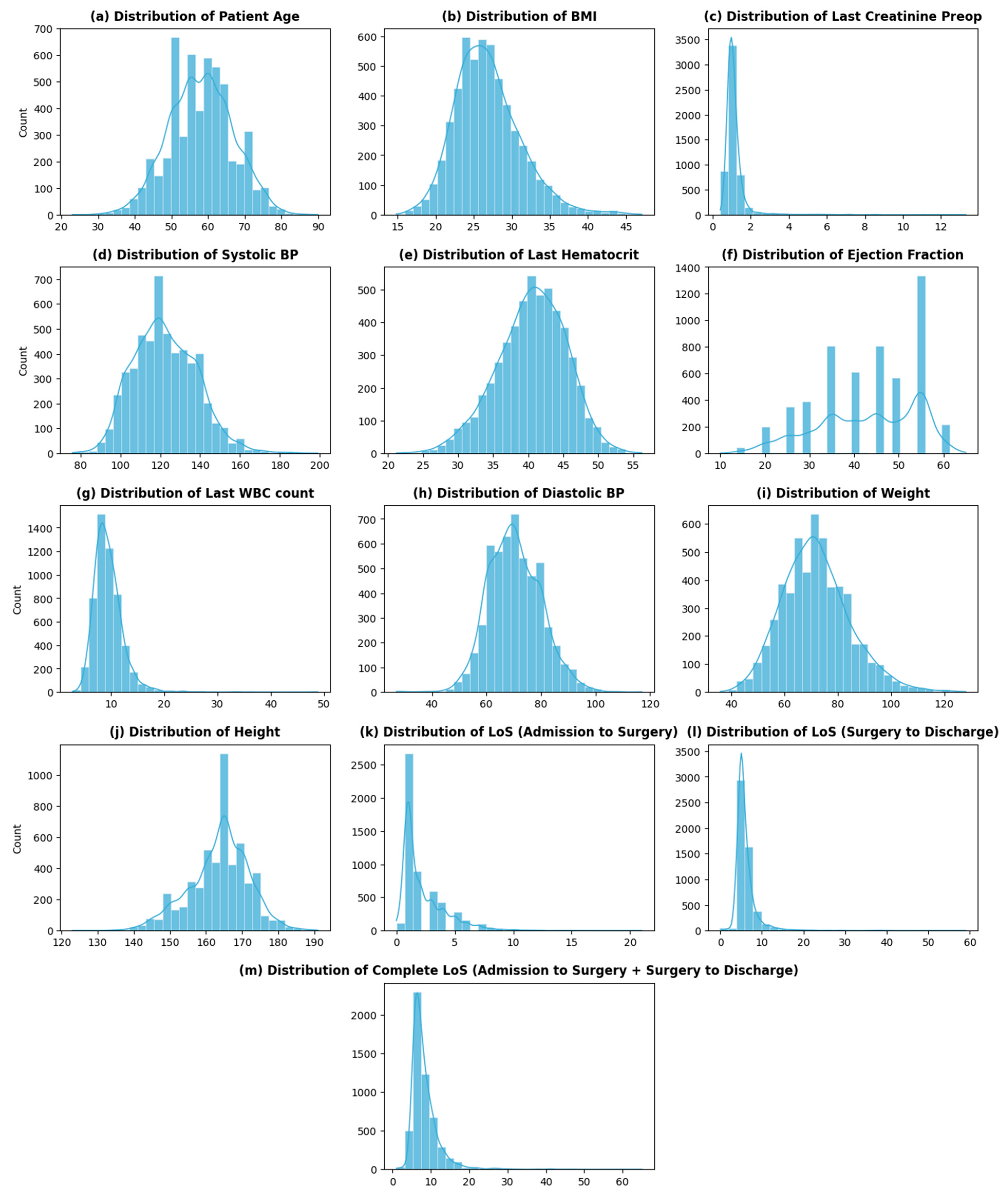
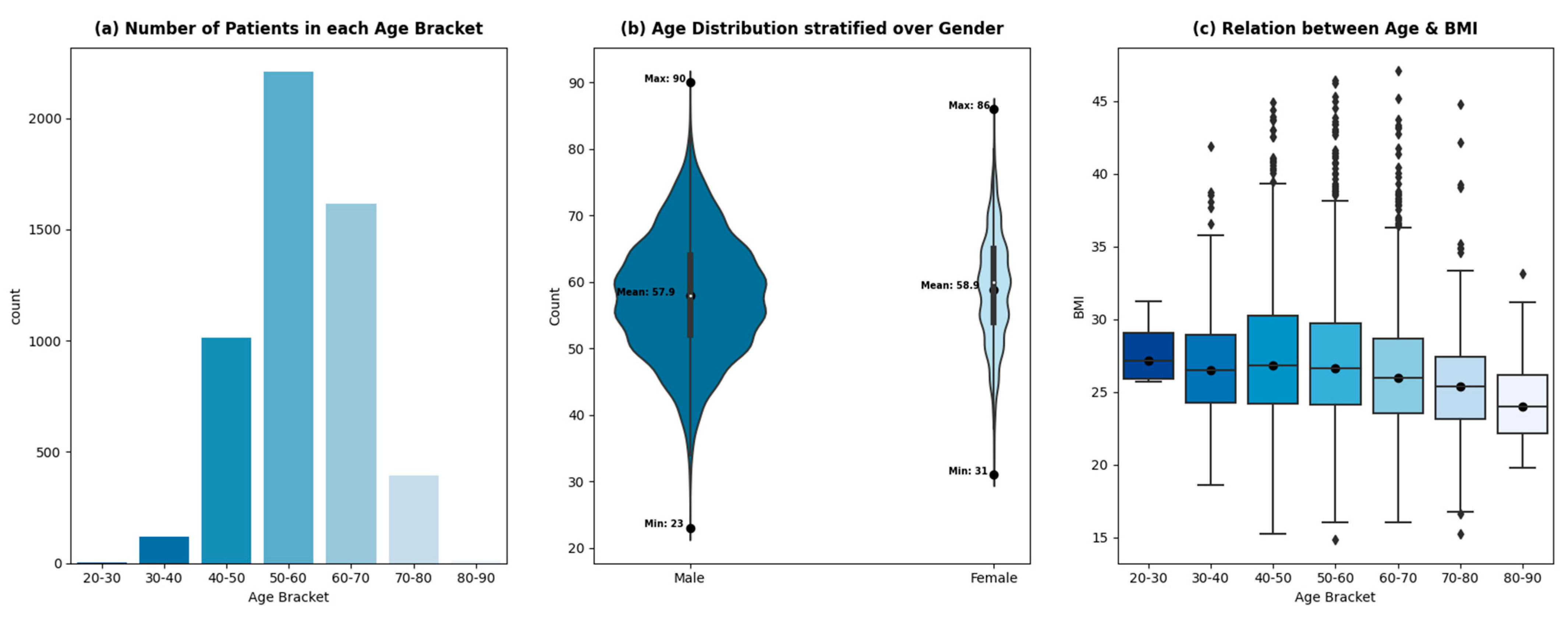
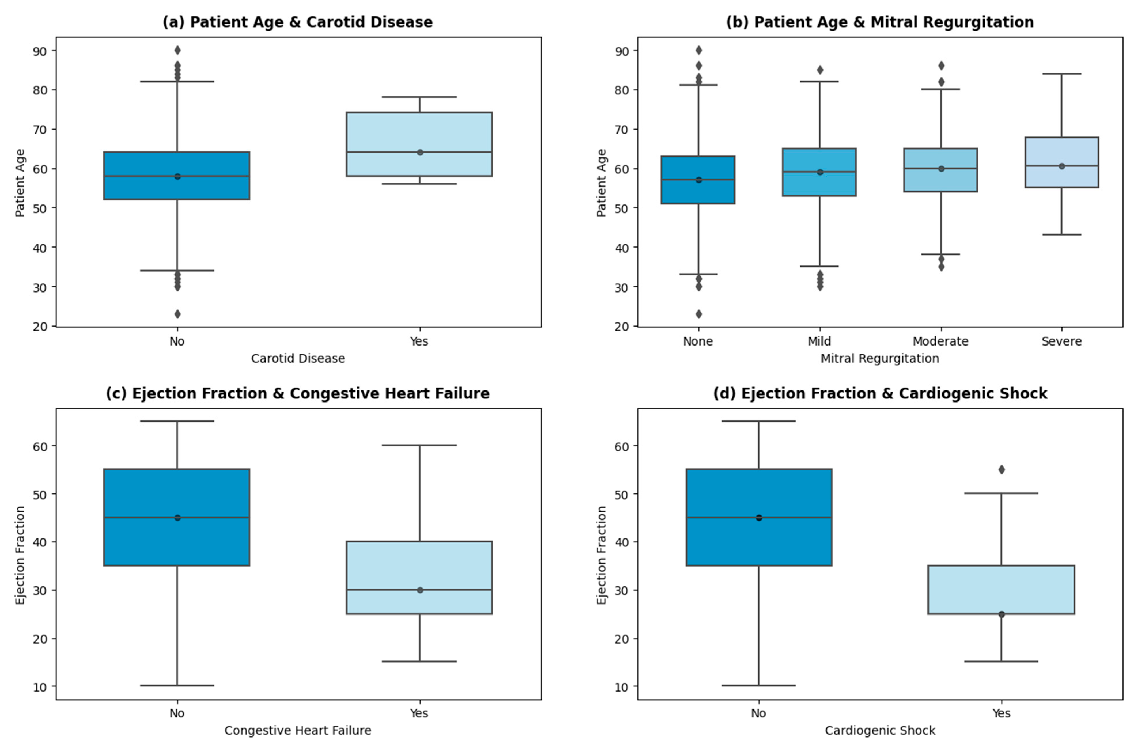
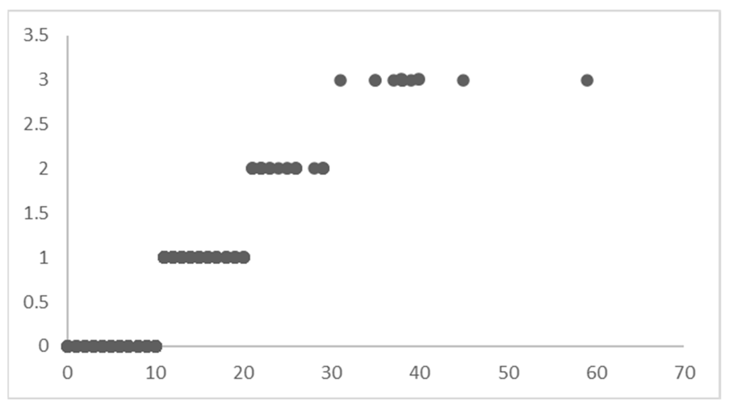
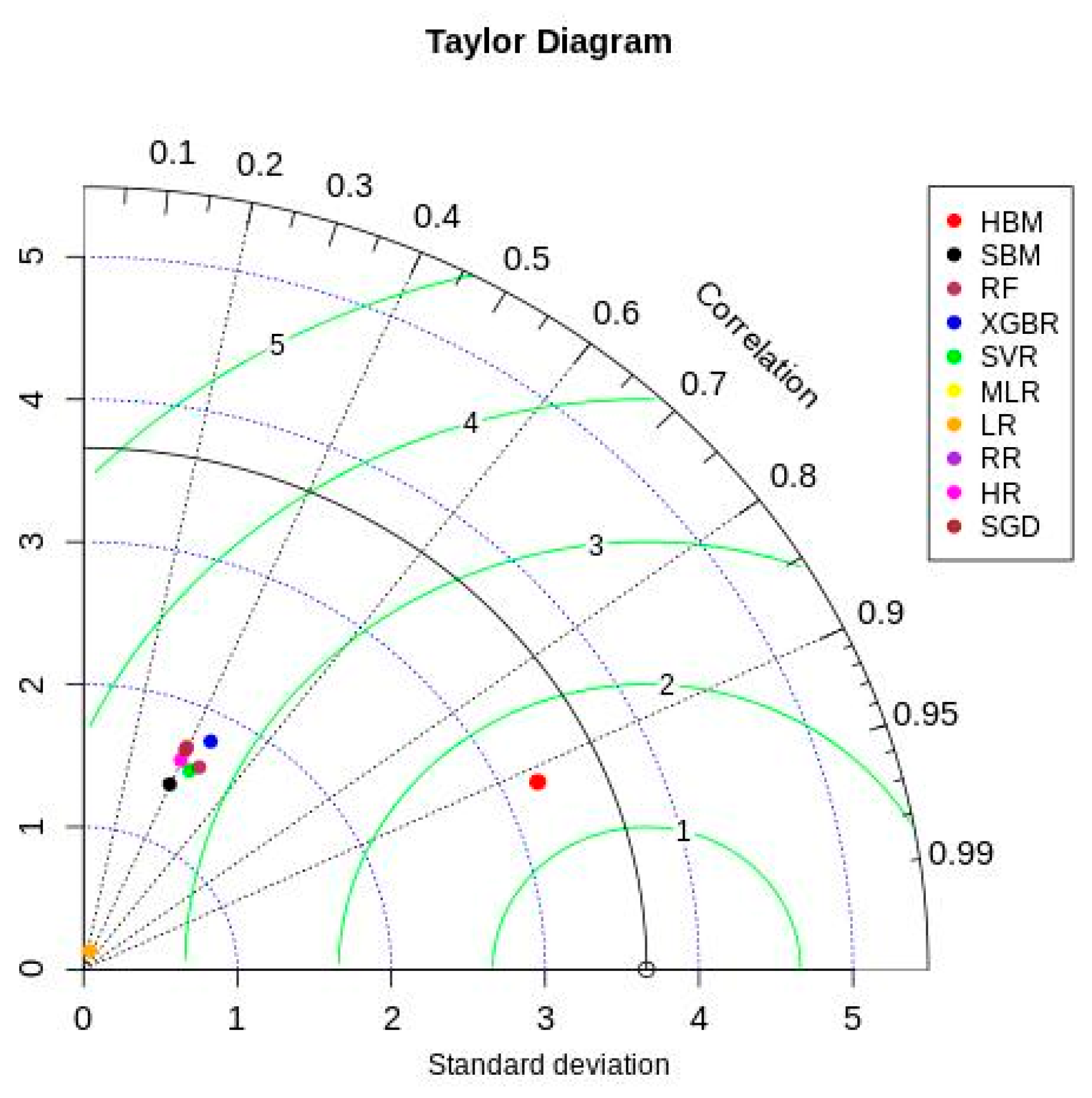
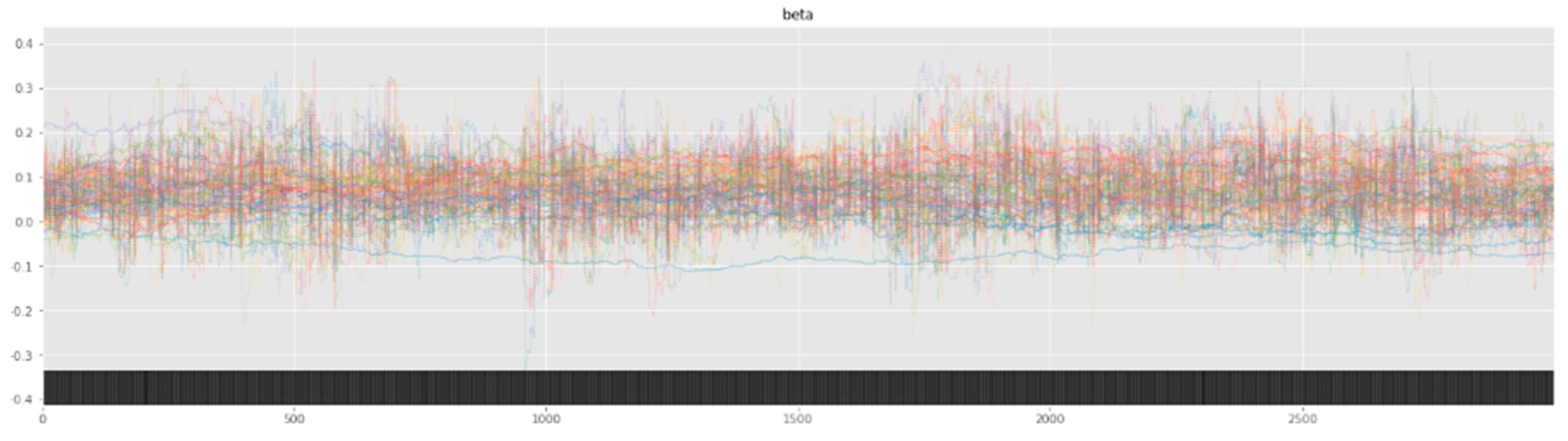
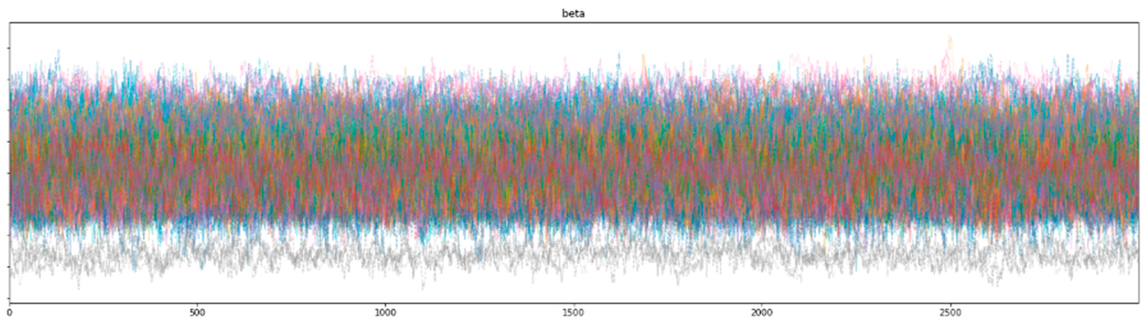
Disclaimer/Publisher’s Note: The statements, opinions and data contained in all publications are solely those of the individual author(s) and contributor(s) and not of MDPI and/or the editor(s). MDPI and/or the editor(s) disclaim responsibility for any injury to people or property resulting from any ideas, methods, instructions or products referred to in the content. |
© 2024 by the authors. Licensee MDPI, Basel, Switzerland. This article is an open access article distributed under the terms and conditions of the Creative Commons Attribution (CC BY) license (https://creativecommons.org/licenses/by/4.0/).