
Bandwidth Improvement in Ultrasound Image Reconstruction Using Deep Learning Techniques

 , ,
, , 
Abstract
1. Introduction
- A DL-based method is proposed for directly transforming a low-bandwidth image reconstruction to a broadband image reconstruction. The transducers are band-limited in nature. The band-limitation of the transducer directly affects the resolution of the US image. This DL based technique can help in transforming the low-bandwidth image reconstruction obtained into a high-bandwidth image reconstruction, which can help in removing artifacts, improving resolution and image quality in general.
- A data driven method was proposed for bandwidth improvement in US imaging for the first-time using DL. The DL model proposed is light weight, has low computational complexity, and can be utilized in real settings. Error analysis, frequency domain comparisons and speckle characteristic comparisons were performed to show the benefits of the proposed method as compared with other state-of-the-art networks.
- A scaled mean square error loss for the training of the DL network is introduced to solve the vanishing gradient problem. The models were trained on only one set of training data and tested on five different datasets with different properties to show the generalizable and scalable property of the proposed model in real settings.
2. Material and Methods
2.1. Deep Learning Techniques
2.1.1. SRCNN
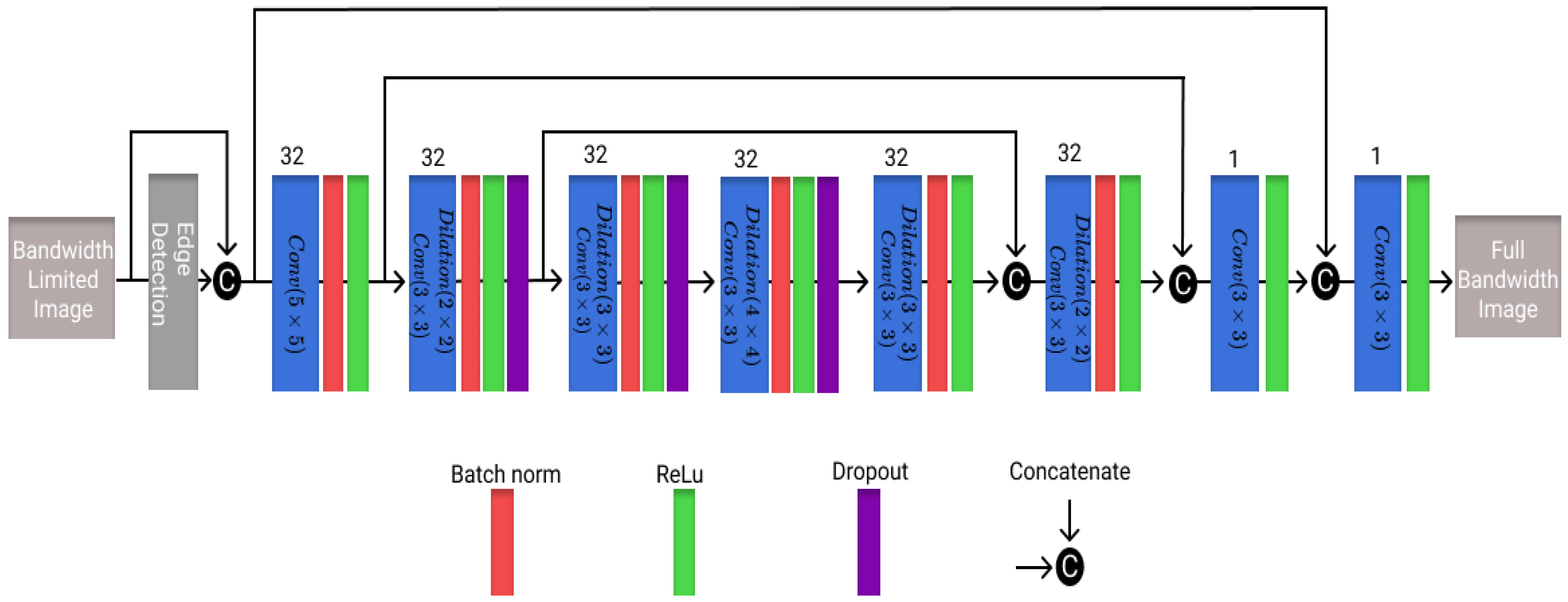
2.1.2. UNet
2.1.3. REDNet
2.2. Loss Functions
- PL1 loss: Scaled mean square error loss. PL1 loss is used as it is more sensitive towards outliers and is the most used loss function [39]. The network was trained using the proposed PL1 (scaled-MSE) loss function, defined as:where, are the predictions of the model, are the true signals and is the scaling factor [40].
2.3. Model Specifications
3. Datasets and Experiments
3.1. Datasets
3.1.1. Phantom I
3.1.2. Phantom II
3.1.3. Commercial Phantom
3.1.4. Carotid Artery
3.1.5. In Vivo Carotid Mimicking Setup
3.2. Experiments
3.2.1. Histogram Equalization (HE)
3.2.2. Contrast Limited Adaptive Histogram Equalization (CLAHE)
- Partitioning of the image into non-overlapping and continuous patches.
- Clipping the histogram of each patch above a threshold and distributing the pixels to all the gray values.
- Applying HE on each patch.
- Interpolating the mapping between separate patches.
4. Figures of Metric
4.1. RMSE
4.2. PSNR
4.3. PC
5. Results
5.1. Results—20% Bandwidth
5.2. Results—40% and 60% Bandwidth
6. Discussion/Analysis of the Results
6.1. Error Analysis
6.2. Frequency Domain Comparison
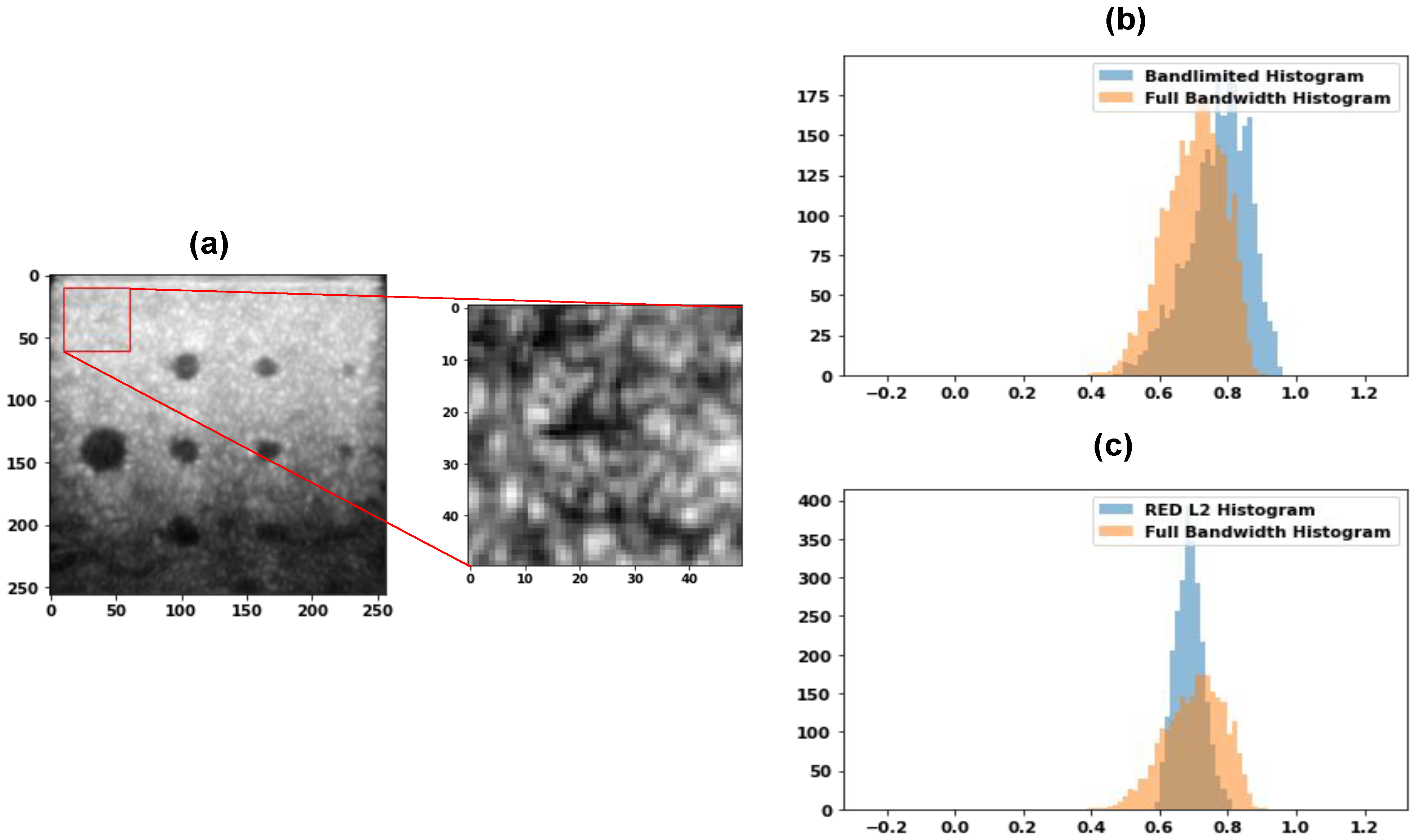
6.3. Histogram Analysis
6.4. Discussion
- Firstly, the amount of bandwidth limitation that can be applied to the full bandwidth data. The bandwidth limited reconstructions sometimes may lose too much information for the model to predict certain structures that were present in the original images. This leads to the complete or partial omission of these structures in the model-enhanced reconstructions, and thus a significantly worse metric score, depending on the dataset and the bandwidth limitation.
- Secondly, the models have trouble in predicting the speckle in US images, which leads to smoothed images in some of the results. The loss of speckle also impacts the usability of the images because the speckle is often used for various diagnostic purposes, for example predicting the type of tissue [61]. Most US machines will have some speckle reduction in post processing. So, this should not be a big problem for normal B-mode imaging, if there is improvement in resolution and quality.
7. Conclusions
Author Contributions
Funding
Institutional Review Board Statement
Informed Consent Statement
Data Availability Statement
Conflicts of Interest
References
- Carovac, A.; Smajlovic, F.; Junuzovic, D. Application of Ultrasound in Medicine. Acta Inform. Medica 2011, 19, 168–171. [Google Scholar] [CrossRef]
- Wells, P.N. Ultrasound imaging. Phys. Med. Biol. 2006, 51, R83. [Google Scholar] [CrossRef] [PubMed]
- Cikes, M.; Tong, L.; Sutherland, G.R.; D’Hooge, J. Ultrafast cardiac ultrasound imaging: Technical principles, applications, and clinical benefits. JACC Cardiovasc. Imaging 2014, 7, 812–823. [Google Scholar] [CrossRef] [PubMed]
- Nicolau, C.; Ripollés, T. Contrast-enhanced ultrasound in abdominal imaging. Abdom. Imaging 2012, 37, 1–19. [Google Scholar] [CrossRef] [PubMed]
- Woo, J. A short history of the development of ultrasound in obstetrics and gynecology. Hist. Ultrasound Obstet. Gynecol. 2002, 3, 1–25. [Google Scholar]
- Szabo, T.L.; Lewin, P.A. Ultrasound transducer selection in clinical imaging practice. J. Ultrasound Med. 2013, 32, 573–582. [Google Scholar] [CrossRef]
- Szabo, T.L. Diagnostic Ultrasound Imaging: Inside Out; Academic Press: New York, NY, USA, 2004. [Google Scholar]
- Szabo, T.L.; Lewin, P.A. Piezoelectric materials for imaging. J. Ultrasound Med. 2007, 26, 283–288. [Google Scholar] [CrossRef][Green Version]
- Reid, J.; Lewin, P. Ultrasound imaging transducers. Encycl. Electr. Electron. Eng. 1999, 22, 664–672. [Google Scholar]
- Maresca, D.; Renaud, G.; van Soest, G.; Li, X.; Zhou, Q.; Shung, K.K.; De Jong, N.; Van der Steen, A.F. Contrast-Enhanced Intravascular Ultrasound Pulse Sequences for Bandwidth-Limited Transducers. Ultrasound Med. Biol. 2013, 39, 706–713. [Google Scholar] [CrossRef]
- Wong, C.M.; Chen, Y.; Luo, H.; Dai, J.; Lam, K.H.; Chan, H.L.W. Development of a 20-MHz wide-bandwidth PMN-PT single crystal phased-array ultrasound transducer. Ultrasonics 2017, 73, 181–186. [Google Scholar] [CrossRef]
- Foster, F.; Zhang, M.; Zhou, Y.; Liu, G.; Mehi, J.; Cherin, E.; Harasiewicz, K.; Starkoski, B.; Zan, L.; Knapik, D.; et al. A new ultrasound instrument for in vivo microimaging of mice. Ultrasound Med. Biol. 2002, 28, 1165–1172. [Google Scholar] [CrossRef] [PubMed]
- Rashid, M.W.; Carpenter, T.; Tekes, C.; Pirouz, A.; Jung, G.; Cowell, D.; Freear, S.; Ghovanloo, M.; Degertekin, F.L. Front-end electronics for cable reduction in Intracardiac Echocardiography (ICE) catheters. In Proceedings of the 2016 IEEE International Ultrasonics Symposium, IUS, Tours, France, 18–21 September 2016. [Google Scholar] [CrossRef]
- Benane, Y.M.; Lavarello, R.; Bujoreanu, D.; Cachard, C.; Varray, F.; Savoia, A.S.; Franceschini, E.; Basset, O. Ultrasound bandwidth enhancement through pulse compression using a CMUT probe. In Proceedings of the 2017 IEEE International Ultrasonics Symposium, IUS, Washington, DC, USA, 6–9 September 2017. [Google Scholar] [CrossRef]
- Costa-Felix, R.; Machado, J.C. Output bandwidth enhancement of a pulsed ultrasound system using a flat envelope and compensated frequency-modulated input signal: Theory and experimental applications. Measurement 2015, 69, 146–154. [Google Scholar] [CrossRef]
- Sainath, T.N.; Kingsbury, B.; Saon, G.; Soltau, H.; Mohamed, A.R.; Dahl, G.; Ramabhadran, B. Deep Convolutional Neural Networks for Large-scale Speech Tasks. Neural Netw. 2015, 64, 39–48. [Google Scholar] [CrossRef] [PubMed]
- Bordes, A.; Chopra, S.; Weston, J. Question answering with subgraph embeddings. In Proceedings of the EMNLP 2014—2014 Conference on Empirical Methods in Natural Language Processing, Doha, Qatar, 25–29 October 2014. [Google Scholar] [CrossRef]
- Rastegari, M.; Ordonez, V.; Redmon, J.; Farhadi, A. XNOR-net: Imagenet classification using binary convolutional neural networks. In Computer Vision—ECCV 2016, Proceedings of the 14th European Conference, Amsterdam, The Netherlands, 11–14 October 2016; Springer: Cham, Switzerland, 2016. [Google Scholar] [CrossRef]
- Minaee, S.; Boykov, Y.Y.; Porikli, F.; Plaza, A.J.; Kehtarnavaz, N.; Terzopoulos, D. Image segmentation using deep learning: A survey. IEEE Trans. Pattern Anal. Mach. Intell. 2022, 44, 3523–3542. [Google Scholar] [CrossRef] [PubMed]
- Zhang, Y.; Li, K.; Li, K.; Zhong, B.; Fu, Y. Residual non-local attention networks for image restoration. In Proceedings of the 7th International Conference on Learning Representations, ICLR 2019, New Orleans, LA, USA, 6–9 May 2019. [Google Scholar]
- Tai, Y.; Yang, J.; Liu, X. Image super-resolution via deep recursive residual network. In Proceedings of the 30th IEEE Conference on Computer Vision and Pattern Recognition, CVPR 2017, Honolulu, HI, USA, 21–26 July 2017. [Google Scholar] [CrossRef]
- Cheng, G.; Matsune, A.; Li, Q.; Zhu, L.; Zang, H.; Zhan, S. Encoder-decoder residual network for real super-resolution. In Proceedings of the IEEE Computer Society Conference on Computer Vision and Pattern Recognition Workshops, Long Beach, CA, USA, 16–17 June 2019. [Google Scholar] [CrossRef]
- Mao, X.J.; Shen, C.; Yang, Y.B. Image restoration using very deep convolutional encoder-decoder networks with symmetric skip connections. In Proceedings of the Advances in Neural Information Processing Systems, Barcelona, Spain, 5–10 December 2016. [Google Scholar]
- Shiri, I.; Akhavanallaf, A.; Sanaat, A.; Salimi, Y.; Askari, D.; Mansouri, Z.; Shayesteh, S.P.; Hasanian, M.; Rezaei-Kalantari, K.; Salahshour, A.; et al. Ultra-low-dose chest CT imaging of COVID-19 patients using a deep residual neural network. Eur. Radiol. 2021, 31, 1420–1431. [Google Scholar] [CrossRef] [PubMed]
- Christensen-Jeffries, K.; Couture, O.; Dayton, P.A.; Eldar, Y.C.; Hynynen, K.; Kiessling, F.; O’Reilly, M.; Pinton, G.F.; Schmitz, G.; Tang, M.X.; et al. Super-resolution ultrasound imaging. Ultrasound Med. Biol. 2020, 46, 865–891. [Google Scholar] [CrossRef]
- Van Sloun, R.J.; Cohen, R.; Eldar, Y.C. Deep learning in ultrasound imaging. Proc. IEEE 2019, 108, 11–29. [Google Scholar] [CrossRef]
- Awasthi, N.; Vermeer, L.; Fixsen, L.S.; Lopata, R.G.; Pluim, J.P. LVNet: Lightweight Model for Left Ventricle Segmentation for Short Axis Views in Echocardiographic Imaging. IEEE Trans. Ultrason. Ferroelectr. Freq. Control 2022, 69, 2115–2128. [Google Scholar] [CrossRef]
- Awasthi, N.; Dayal, A.; Cenkeramaddi, L.R.; Yalavarthy, P.K. Mini-COVIDNet: Efficient lightweight deep neural network for ultrasound based point-of-care detection of COVID-19. IEEE Trans. Ultrason. Ferroelectr. Freq. Control 2021, 68, 2023–2037. [Google Scholar] [CrossRef]
- Chaudhari, A.S.; Fang, Z.; Kogan, F.; Wood, J.; Stevens, K.J.; Gibbons, E.K.; Lee, J.H.; Gold, G.E.; Hargreaves, B.A. Super-resolution musculoskeletal MRI using deep learning. Magn. Reson. Med. 2018, 80, 2139–2154. [Google Scholar] [CrossRef]
- Chun, J.; Zhang, H.; Gach, H.M.; Olberg, S.; Mazur, T.; Green, O.; Kim, T.; Kim, H.; Kim, J.S.; Mutic, S.; et al. MRI super-resolution reconstruction for MRI-guided adaptive radiotherapy using cascaded deep learning: In the presence of limited training data and unknown translation model. Med. Phys. 2019, 46, 4148–4164. [Google Scholar] [CrossRef] [PubMed]
- Perdios, D.; Vonlanthen, M.; Martinez, F.; Arditi, M.; Thiran, J.P. CNN-based image reconstruction method for ultrafast ultrasound imaging. IEEE Trans. Ultrason. Ferroelectr. Freq. Control 2021, 69, 1154–1168. [Google Scholar] [CrossRef] [PubMed]
- Yoon, Y.H.; Khan, S.; Huh, J.; Ye, J.C. Efficient B-Mode Ultrasound Image Reconstruction From Sub-Sampled RF Data Using Deep Learning. IEEE Trans. Med. Imaging 2019, 38, 325–336. [Google Scholar] [CrossRef] [PubMed]
- Dong, C.; Loy, C.C.; He, K.; Tang, X. Image Super-Resolution Using Deep Convolutional Networks. IEEE Trans. Pattern Anal. Mach. Intell. 2016, 38, 295–307. [Google Scholar] [CrossRef] [PubMed]
- Ronneberger, O.; Fischer, P.; Brox, T. U-net: Convolutional networks for biomedical image segmentation. In Medical Image Computing and Computer-Assisted Intervention, Proceedings of the MICCAI 2015—18th International Conference, Munich, Germany, 5–9 October 2015; Springer: Cham, Switzerland, 2015. [Google Scholar] [CrossRef]
- Gholizadeh-Ansari, M.; Alirezaie, J.; Babyn, P. Deep learning for low-dose CT denoising using perceptual loss and edge detection layer. J. Digit. Imaging 2020, 33, 504–515. [Google Scholar] [CrossRef] [PubMed]
- Heinrich, M.P.; Stille, M.; Buzug, T.M. Residual U-Net convolutional neural network architecture for low-dose CT denoising. Curr. Dir. Biomed. Eng. 2018, 4, 297–300. [Google Scholar] [CrossRef]
- Awasthi, N.; Jain, G.; Kalva, S.K.; Pramanik, M.; Yalavarthy, P.K. Deep neural network-based sinogram super-resolution and bandwidth enhancement for limited-data photoacoustic tomography. IEEE Trans. Ultrason. Ferroelectr. Freq. Control 2020, 67, 2660–2673. [Google Scholar] [CrossRef]
- Zhang, K.; Zuo, W.; Gu, S.; Zhang, L. Learning deep CNN denoiser prior for image restoration. In Proceedings of the 30th IEEE Conference on Computer Vision and Pattern Recognition, CVPR 2017, Honolulu, HI, USA, 21–26 July 2017. [Google Scholar] [CrossRef]
- Wang, Q.; Ma, Y.; Zhao, K.; Tian, Y. A comprehensive survey of loss functions in machine learning. Ann. Data Sci. 2022, 9, 187–212. [Google Scholar] [CrossRef]
- Micikevicius, P.; Narang, S.; Alben, J.; Diamos, G.; Elsen, E.; Garcia, D.; Ginsburg, B.; Houston, M.; Kuchaiev, O.; Venkatesh, G.; et al. Mixed precision training. arXiv 2017, arXiv:1710.03740. [Google Scholar]
- Abadi, M.; Agarwal, A.; Barham, P.; Brevdo, E.; Chen, Z.; Citro, C.; Corrado, G.S.; Davis, A.; Dean, J.; Devin, M.; et al. TensorFlow: Large-Scale Machine Learning on Heterogeneous Systems, 2015. Software. Available online: https://tensorflow.org (accessed on 1 March 2021).
- Chollet, F. Keras. 2015. Available online: https://keras.io (accessed on 1 March 2021).
- Kingma, D.P.; Ba, J. Adam: A method for stochastic optimization. arXiv 2014, arXiv:1412.6980. [Google Scholar]
- Jansen, G.; Awasthi, N.; Schwab, H.M.; Lopata, R. Enhanced Radon Domain Beamforming Using Deep-Learning-Based Plane Wave Compounding. In Proceedings of the 2021 IEEE International Ultrasonics Symposium (IUS), Xi’an, China, 11–16 September 2021; pp. 1–4. [Google Scholar]
- Parker, N.; Povey, M. Ultrasonic study of the gelation of gelatin: Phase diagram, hysteresis and kinetics. Food Hydrocoll. 2012, 26, 99–107. [Google Scholar] [CrossRef]
- Li, Y.; Wang, W.; Yu, D. Application of adaptive histogram equalization to X-ray chest images. In Proceedings of the Second International Conference on Optoelectronic Science and Engineering’94, Beijing, China, 15–18 August 1994; Volume 2321, pp. 513–514. [Google Scholar]
- Zimmerman, J.B.; Pizer, S.M.; Staab, E.V.; Perry, J.R.; McCartney, W.; Brenton, B.C. An evaluation of the effectiveness of adaptive histogram equalization for contrast enhancement. IEEE Trans. Med. Imaging 1988, 7, 304–312. [Google Scholar] [CrossRef] [PubMed]
- Lim, J.S. Two-Dimensional Signal and Image Processing; Prentice Hall: Englewood Cliffs, NJ, USA, 1990. [Google Scholar]
- Gonzalez, R.C.; Woods, R.E. Digital Image Processing; Pearson Education (Singapore) Pte. Ltd.: Delhi, India, 2002. [Google Scholar]
- Kim, Y.T. Contrast enhancement using brightness preserving bi-histogram equalization. IEEE Trans. Consum. Electron. 1997, 43, 1–8. [Google Scholar]
- Zuiderveld, K. Contrast limited adaptive histogram equalization. In Graphics Gems; Academic Press Professional, Inc.: Cambridge, MA, USA, 1994; pp. 474–485. [Google Scholar]
- Pai, P.P.; De, A.; Banerjee, S. Accuracy enhancement for noninvasive glucose estimation using dual-wavelength photoacoustic measurements and kernel-based calibration. IEEE Trans. Instrum. Meas. 2018, 67, 126–136. [Google Scholar] [CrossRef]
- Horé, A.; Ziou, D. Image quality metrics: PSNR vs. SSIM. In Proceedings of the 2010 International Conference on Pattern Recognition, Istanbul, Turkey, 23–26 August 2010. [Google Scholar] [CrossRef]
- Awasthi, N.; Kalva, S.K.; Pramanik, M.; Yalavarthy, P.K. Dimensionality reduced plug and play priors for improving photoacoustic tomographic imaging with limited noisy data. Biomed. Opt. Express 2021, 12, 1320–1338. [Google Scholar] [CrossRef]
- Benesty, J.; Chen, J.; Huang, Y.; Cohen, I. Pearson correlation coefficient. In Noise Reduction in Speech Processing; Springer: Berlin/Heidelberg, Germany, 2009; pp. 1–4. [Google Scholar]
- Yang, X.; Wang, S.; Han, J.; Guo, Y.; Li, T. RSAMSR: A deep neural network based on residual self-encoding and attention mechanism for image super-resolution. Optik 2021, 245, 167736. [Google Scholar] [CrossRef]
- Yang, X.; Zhu, Y.; Guo, Y.; Zhou, D. An image super-resolution network based on multi-scale convolution fusion. Vis. Comput. 2022, 38, 4307–4317. [Google Scholar] [CrossRef]
- Yang, X.; Fan, J.; Wu, C.; Zhou, D.; Li, T. NasmamSR: A fast image super-resolution network based on neural architecture search and multiple attention mechanism. Multimed. Syst. 2022, 28, 321–334. [Google Scholar] [CrossRef]
- Xu, J.; Zhou, W.; Chen, Z.; Ling, S.; Le Callet, P. Binocular rivalry oriented predictive autoencoding network for blind stereoscopic image quality measurement. IEEE Trans. Instrum. Meas. 2020, 70, 1–13. [Google Scholar] [CrossRef]
- Mishra, D.; Singh, S.K.; Singh, R.K. Wavelet-based deep auto encoder-decoder (wdaed)-based image compression. IEEE Trans. Circuits Syst. Video Technol. 2020, 31, 1452–1462. [Google Scholar] [CrossRef]
- Damerjian, V.; Tankyevych, O.; Souag, N.; Petit, E. Speckle characterization methods in ultrasound images—A review. IRBM 2014, 35, 202–213. [Google Scholar] [CrossRef]
- Sajjadi, M.S.; Scholkopf, B.; Hirsch, M. EnhanceNet: Single image super-resolution through automated texture synthesis. In Proceedings of the 2017 IEEE International Conference on Computer Vision, Venice, Italy, 22–29 October 2017. [Google Scholar] [CrossRef]
- Agostinelli, F.; Anderson, M.R.; Lee, H. Adaptive multi-column deep neural networks with application to robust image denoising. In Proceedings of the Advances in Neural Information Processing Systems 2013, Lake Tahoe, NV, USA, 5–10 December 2013. [Google Scholar]


| Dataset | Train | Validation | Test |
|---|---|---|---|
| Phantom I | 400 | 135 | 134 |
| Phantom II | - | - | 90 |
| Commercial phantom | - | - | 31 |
| Carotid artery | - | - | 70 |
| In vivo carotid mimicking setup | - | - | 239 |
| Dataset | Model | 20% Bandwidth | 40% Bandwidth | 60% Bandwidth | |||
|---|---|---|---|---|---|---|---|
| RMSE | PSNR | RMSE | PSNR | RMSE | PSNR | ||
| Phantom I | Bandwidth limited | 0.141 ± 0.016 | 17.049 ± 1.017 | 0.106 ± 0.012 | 19.590 ± 1.010 | 0.080 ± 0.010 | 21.953 ± 1.111 |
| HE | 0.297 ± 0.044 | 10.642 ± 1.316 | 0.280 ± 0.040 | 11.156 ± 1.296 | 0.265 ± 0.039 | 11.632 ± 1.331 | |
| CLAHE | 0.344 ± 0.037 | 9.331 ± 0.948 | 0.324 ± 0.033 | 9.838 ± 0.908 | 0.307 ± 0.032 | 10.305 ± 0.928 | |
| PL1(U-Net) | 0.097 ± 0.012 | 20.311 ± 1.123 | 0.134 ± 0.040 | 17.777 ± 2.387 | 0.091 ± 0.027 | 21.132 ± 2.296 | |
| PL2(U-Net) | 0.581 ± 0.325 | 6.140 ± 5.145 | 0.667 ± 0.246 | 4.298 ± 4.030 | 0.083 ± 0.013 | 21.764 ± 1.328 | |
| PL1(SRCNN) | 0.093 ± 0.012 | 20.683 ± 1.129 | 0.106 ± 0.011 | 19.590 ± 1.010 | 0.062 ± 0.009 | 24.276 ± 1.296 | |
| PL2(SRCNN) | 0.131 ± 0.015 | 17.690 ± 0.915 | 0.108 ± 0.016 | 19.384 ± 1.208 | 0.080 ± 0.013 | 22.014 ± 1.428 | |
| PL1(RED) | 0.091 ± 0.012 | 20.903 ± 1.189 | 0.077 ± 0.010 | 22.369 ± 1.219 | 0.059 ± 0.008 | 24.661 ± 1.302 | |
| PL2(RED) | 0.116 ± 0.013 | 18.802 ± 0.956 | 0.092 ± 0.014 | 20.839 ± 1.279 | 0.072 ± 0.012 | 22.978 ± 1.442 | |
| Carotid artery | Bandwidth limited | 0.165 ± 0.026 | 15.768 ± 1.376 | 0.110 ± 0.018 | 19.266 ± 1.359 | 0.084 ± 0.013 | 21.577 ± 1.327 |
| HE | 0.313 ± 0.030 | 10.131 ± 0.856 | 0.269 ± 0.026 | 11.451 ± 0.862 | 0.242 ± 0.023 | 12.348 ± 0.836 | |
| CLAHE | 0.344 ± 0.028 | 9.310 ± 0.733 | 0.298 ± 0.026 | 10.557 ± 0.761 | 0.270 ± 0.023 | 11.395 ± 0.753 | |
| PL1(U-Net) | 0.096 ± 0.015 | 20.446 ± 1.378 | 0.236 ± 0.020 | 12.560 ± 0.757 | 0.169 ± 0.018 | 15.490 ± 0.901 | |
| PL2(U-Net) | 0.247 ± 0.121 | 13.010 ± 3.674 | 0.806 ± 0.088 | 1.927 ± 0.955 | 0.088 ± 0.005 | 21.120 ± 0.512 | |
| PL1(SRCNN) | 0.107 ± 0.013 | 19.477 ± 1.162 | 0.080 ± 0.012 | 22.002 ± 1.318 | 0.066 ± 0.010 | 23.657 ± 1.381 | |
| PL2(SRCNN) | 0.151 ± 0.007 | 16.435 ± 0.408 | 0.112 ± 0.008 | 19.028 ± 0.606 | 0.082 ± 0.008 | 21.786 ± 0.890 | |
| PL1(RED) | 0.095 ± 0.013 | 20.523 ± 1.242 | 0.077 ± 0.011 | 22.399 ± 1.333 | 0.063 ± 0.010 | 24.134 ± 1.471 | |
| PL2(RED) | 0.125 ± 0.008 | 18.110 ± 0.608 | 0.093 ± 0.009 | 20.655 ± 0.858 | 0.074 ± 0.008 | 22.716 ± 0.960 | |
| Commercial phantom | Bandwidth limited | 0.204 ± 0.032 | 13.885 ± 1.276 | 0.195 ± 0.040 | 14.390 ± 1.724 | 0.187 ± 0.049 | 14.874 ± 2.363 |
| HE | 0.236 ± 0.024 | 12.586 ± 0.840 | 0.229 ± 0.030 | 12.863 ± 1.130 | 0.226 ± 0.035 | 13.039 ± 1.366 | |
| CLAHE | 0.287 ± 0.023 | 10.871 ± 0.674 | 0.282 ± 0.027 | 11.017 ± 0.823 | 0.279 ± 0.031 | 11.130 ± 0.967 | |
| PL1(U-Net) | 0.197 ± 0.020 | 14.146 ± 0.884 | 0.210 ± 0.032 | 13.638 ± 1.359 | 0.187 ± 0.041 | 14.814 ± 2.115 | |
| PL2(U-Net) | 0.421 ± 0.095 | 7.736 ± 1.983 | 0.467 ± 0.070 | 6.720 ± 1.340 | 0.338 ± 0.357 | 12.348 ± 6.212 | |
| PL1(SRCNN) | 0.202 ± 0.025 | 13.956 ± 1.110 | 0.192 ± 0.018 | 14.354 ± 0.800 | 0.183 ± 0.032 | 14.876 ± 1.600 | |
| PL2(SRCNN) | 0.223 ± 0.063 | 13.429 ± 2.717 | 0.217 ± 0.045 | 13.483 ± 1.915 | 0.188 ± 0.030 | 14.623 ± 1.338 | |
| PL1(RED) | 0.201 ± 0.025 | 13.985 ± 1.120 | 0.191 ± 0.019 | 14.410 ± 0.844 | 0.182 ± 0.037 | 14.968 ± 1.866 | |
| PL2(RED) | 0.204 ± 0.061 | 14.242 ± 2.894 | 0.193 ± 0.047 | 14.575 ± 2.238 | 0.179 ± 0.026 | 15.013 ± 1.217 | |
| Phantom II | Bandwidth limited | 0.155 ± 0.021 | 16.297 ± 1.212 | 0.100 ± 0.012 | 20.044 ± 1.132 | 0.074 ± 0.009 | 22.690 ± 1.201 |
| HE | 0.318 ± 0.032 | 9.994 ± 0.936 | 0.282 ± 0.025 | 11.021 ± 0.815 | 0.260 ± 0.022 | 11.742 ± 0.778 | |
| CLAHE | 0.355 ± 0.027 | 9.017 ± 0.672 | 0.317 ± 0.023 | 10.007 ± 0.634 | 0.294 ± 0.022 | 10.672 ± 0.662 | |
| PL1(U-Net) | 0.089 ± 0.012 | 21.086 ± 1.217 | 0.207 ± 0.040 | 13.869 ± 1.874 | 0.146 ± 0.030 | 16.932 ± 1.910 | |
| PL2(U-Net) | 0.393 ± 0.210 | 9.334 ± 4.655 | 0.854 ± 0.173 | 1.566 ± 1.929 | 0.081 ± 0.006 | 21.862 ± 0.669 | |
| PL1(SRCNN) | 0.096 ± 0.011 | 20.427 ± 1.067 | 0.069 ± 0.010 | 23.331 ± 1.248 | 0.054 ± 0.008 | 25.395 ± 1.270 | |
| PL2(SRCNN) | 0.144 ± 0.013 | 16.855 ± 0.767 | 0.106 ± 0.009 | 19.513 ± 0.709 | 0.074 ± 0.009 | 22.646 ± 0.984 | |
| PL1(RED) | 0.085 ± 0.012 | 21.457 ± 1.238 | 0.065 ± 0.010 | 23.790 ± 1.368 | 0.051 ± 0.007 | 25.975 ± 1.274 | |
| PL2(RED) | 0.119 ± 0.009 | 18.506 ± 0.630 | 0.087 ± 0.009 | 21.245 ± 0.899 | 0.067 ± 0.009 | 23.577 ± 1.099 | |
| In vivo carotid mimicking setup | Bandwidth limited | 0.172 ± 0.040 | 15.487 ± 1.876 | 0.134 ± 0.027 | 17.591 ± 1.695 | 0.110 ± 0.018 | 19.274 ± 1.482 |
| HE | 0.276 ± 0.042 | 11.271 ± 1.303 | 0.254 ± 0.039 | 11.984 ± 1.302 | 0.244 ± 0.036 | 12.361 ± 1.285 | |
| CLAHE | 0.302 ± 0.038 | 10.482 ± 1.090 | 0.276 ± 0.036 | 11.257 ± 1.113 | 0.266 ± 0.033 | 11.554 ± 1.065 | |
| PL1(U-Net) | 0.143 ± 0.027 | 17.081 ± 1.680 | 0.250 ± 0.028 | 12.103 ± 0.976 | 0.177 ± 0.023 | 15.127 ± 1.134 | |
| PL2(U-Net) | 0.199 ± 0.078 | 14.522 ± 2.834 | 0.736 ± 0.087 | 2.723 ± 0.995 | 0.100 ± 0.013 | 20.094 ± 1.097 | |
| PL1(SRCNN) | 0.135 ± 0.023 | 17.558 ± 1.544 | 0.117 ± 0.019 | 18.775 ± 1.477 | 0.100 ± 0.016 | 20.134 ± 1.487 | |
| PL2(SRCNN) | 0.148 ± 0.013 | 16.602 ± 0.719 | 0.130 ± 0.017 | 17.784 ± 1.130 | 0.104 ± 0.016 | 19.795 ± 1.400 | |
| PL1(RED) | 0.133 ± 0.022 | 17.654 ± 1.536 | 0.118 ± 0.019 | 18.710 ± 1.476 | 0.098 ± 0.016 | 20.340 ± 1.553 | |
| PL2(RED) | 0.130 ± 0.015 | 17.787 ± 0.975 | 0.111 ± 0.017 | 19.204 ± 1.316 | 0.096 ± 0.015 | 20.485 ± 1.424 | |
| Dataset | Bandwidth | RMSE (%) | PSNR (dB) |
|---|---|---|---|
| Phantom I | 20% | 35.46 | 3.85 |
| 40% | 27.35 | 2.77 | |
| 60% | 26.25 | 2.70 | |
| Carotid artery | 20% | 42.42 | 4.76 |
| 40% | 30.00 | 3.13 | |
| 60% | 25.00 | 2.56 | |
| Commercial phantom | 20% | 3.43 | 0.36 |
| 40% | 2.05 | 0.18 | |
| 60% | 4.28 | 0.14 | |
| Phantom II | 20% | 45.16 | 5.16 |
| 40% | 35.00 | 3.75 | |
| 60% | 31.08 | 3.28 | |
| In vivo carotid mimicking setup | 20% | 24.24 | 2.30 |
| 40% | 17.16 | 1.61 | |
| 60% | 12.72 | 1.21 |
| Model | Total Parameters | Trainable Parameters | Non-Trainable Parameters | Model Size (MB) |
|---|---|---|---|---|
| SRCNN | 85,889 | 85,889 | 0 | 1.06 |
| U-Net | 2,164,433 | 2,161,489 | 2944 | 26.3 |
| REDNet | 60,760 | 60,440 | 320 | 0.87 |
Disclaimer/Publisher’s Note: The statements, opinions and data contained in all publications are solely those of the individual author(s) and contributor(s) and not of MDPI and/or the editor(s). MDPI and/or the editor(s) disclaim responsibility for any injury to people or property resulting from any ideas, methods, instructions or products referred to in the content. |
© 2022 by the authors. Licensee MDPI, Basel, Switzerland. This article is an open access article distributed under the terms and conditions of the Creative Commons Attribution (CC BY) license (https://creativecommons.org/licenses/by/4.0/).
Share and Cite
Awasthi, N.; van Anrooij, L.; Jansen, G.; Schwab, H.-M.; Pluim, J.P.W.; Lopata, R.G.P. Bandwidth Improvement in Ultrasound Image Reconstruction Using Deep Learning Techniques. Healthcare 2023, 11, 123. https://doi.org/10.3390/healthcare11010123
Awasthi N, van Anrooij L, Jansen G, Schwab H-M, Pluim JPW, Lopata RGP. Bandwidth Improvement in Ultrasound Image Reconstruction Using Deep Learning Techniques. Healthcare. 2023; 11(1):123. https://doi.org/10.3390/healthcare11010123
Chicago/Turabian StyleAwasthi, Navchetan, Laslo van Anrooij, Gino Jansen, Hans-Martin Schwab, Josien P. W. Pluim, and Richard G. P. Lopata. 2023. "Bandwidth Improvement in Ultrasound Image Reconstruction Using Deep Learning Techniques" Healthcare 11, no. 1: 123. https://doi.org/10.3390/healthcare11010123
APA StyleAwasthi, N., van Anrooij, L., Jansen, G., Schwab, H.-M., Pluim, J. P. W., & Lopata, R. G. P. (2023). Bandwidth Improvement in Ultrasound Image Reconstruction Using Deep Learning Techniques. Healthcare, 11(1), 123. https://doi.org/10.3390/healthcare11010123