
Cluster Analysis of US COVID-19 Infected States for Vaccine Distribution


Abstract
:1. Introduction
2. Preliminary
2.1. COVID-19
2.2. Medical Indicators and Vaccine Allocation
2.3. Feature Selection Techniques
2.3.1. Principal Component Analysis (PCA)
| Algorithm 1 PCA based Feature Selection. | |
| Inputs: X = {x1, x2, ……, xD} // D-dimension training dataset | |
| Outputs: Y = {y1, y2, ……, yd} // lower dimensionality d-dimensional feature set where d <= D | |
| 1 | Do PCA on X for dimensionality reduction |
| 2 | Compute mean of input dataset (x)’ |
| 3 | Calculate the covariance matrix Cov (x) |
| 4 | Find spectral decomposition of Cov (x) and the corresponding Eigen vectors and values E1, E2, …ED to get the principal components P = (x1′, x2′, ……, xn′) which is a subset of X. |
2.3.2. Information Gain
| Algorithm 2 Information gain-based feature selection | |
| Inputs: Dataset D | |
| Outputs: Selected Features FS | |
| 1 | Start |
| 2 | Initialize threshold for gain gt |
| 3 | Initialize feature -gain map G |
| 4 | Get attributes from D into A provided c |
| 5 | for each attribute a in A |
| 6 | Find gain g |
| 7 | IF (g > gt) THEN |
| 8 | Add attribute a and g to G |
| 9 | End IF |
| 10 | End For |
| 11 | For each element in G |
| 12 | IF feature is found useful THEN |
| 13 | Update FS with the feature |
| 14 | END IF |
2.3.3. Gain Ratio
2.4. Cluster Analysis
2.4.1. K-Means
2.4.2. Cascade K-Means
2.5. Classification
2.5.1. Random Forest
- Sample, with replacement, n training examples from X, Y; call these Xb, Yb.
- Train a classification or regression tree fb on Xb, Yb.
2.5.2. Neural Network
3. Material and Methods
3.1. Dataset
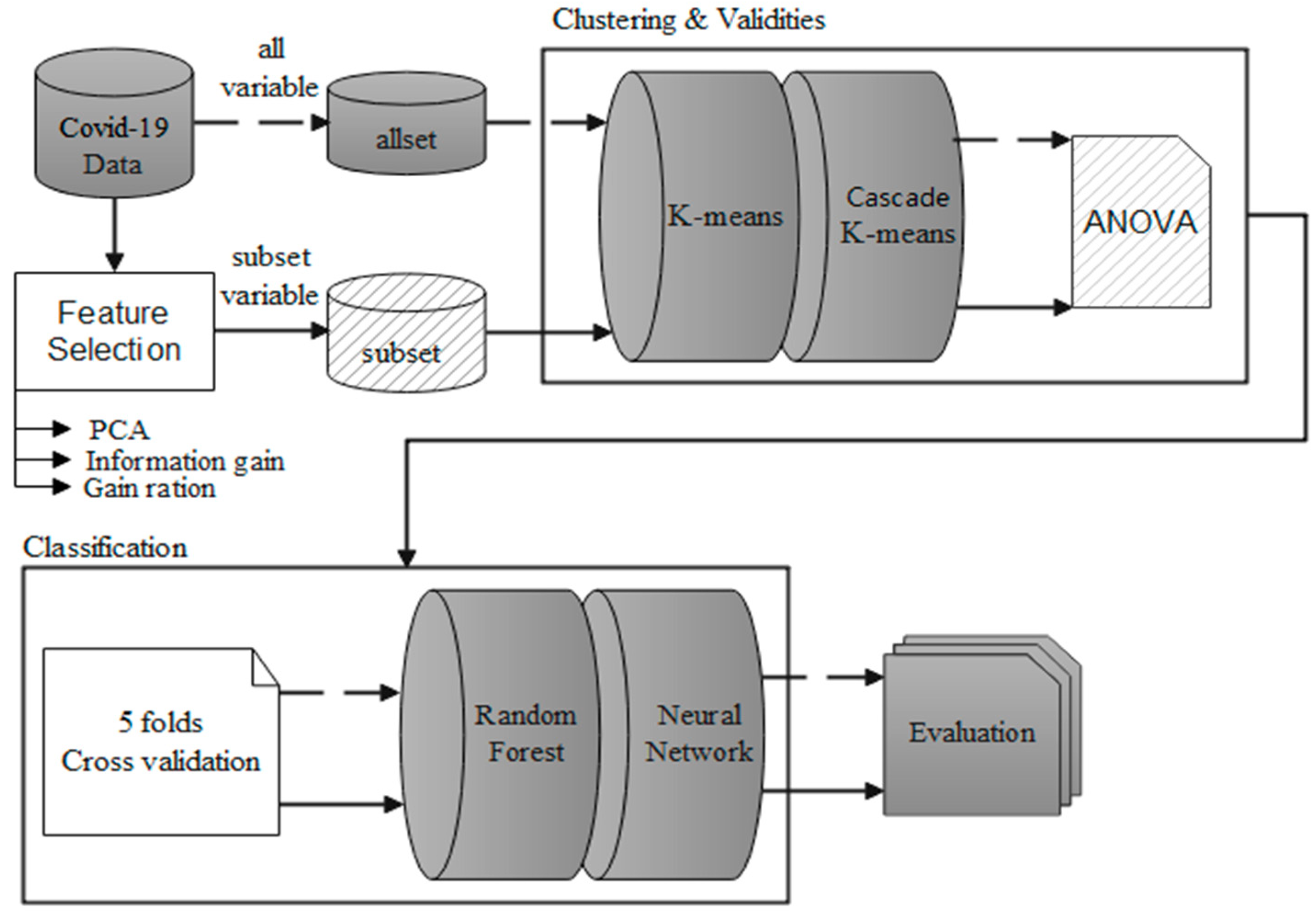
3.2. Conceptual Framework
3.3. A Brief Review of Clustering Techniques
3.4. Data Preprocessing
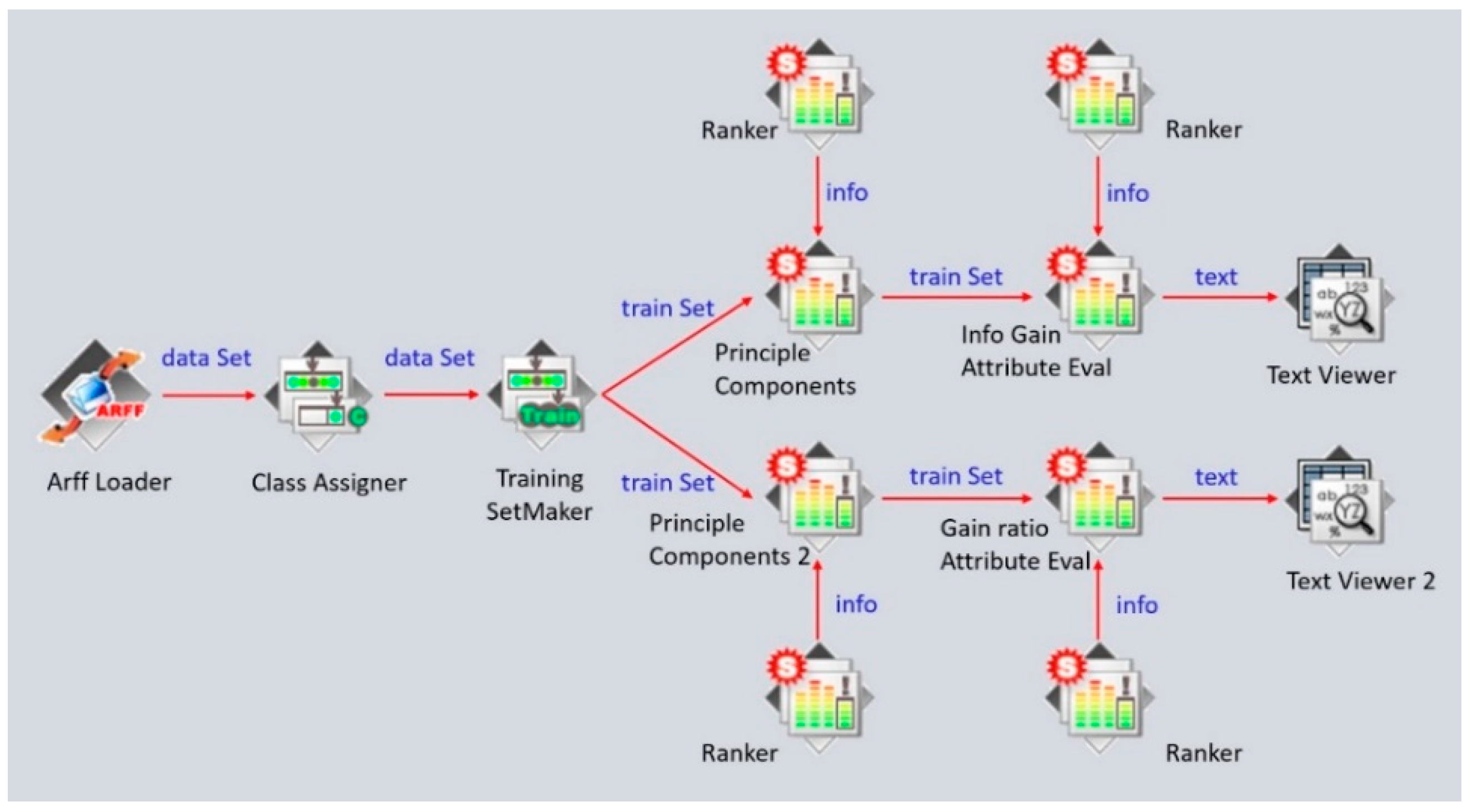
3.4.1. Feature Selection
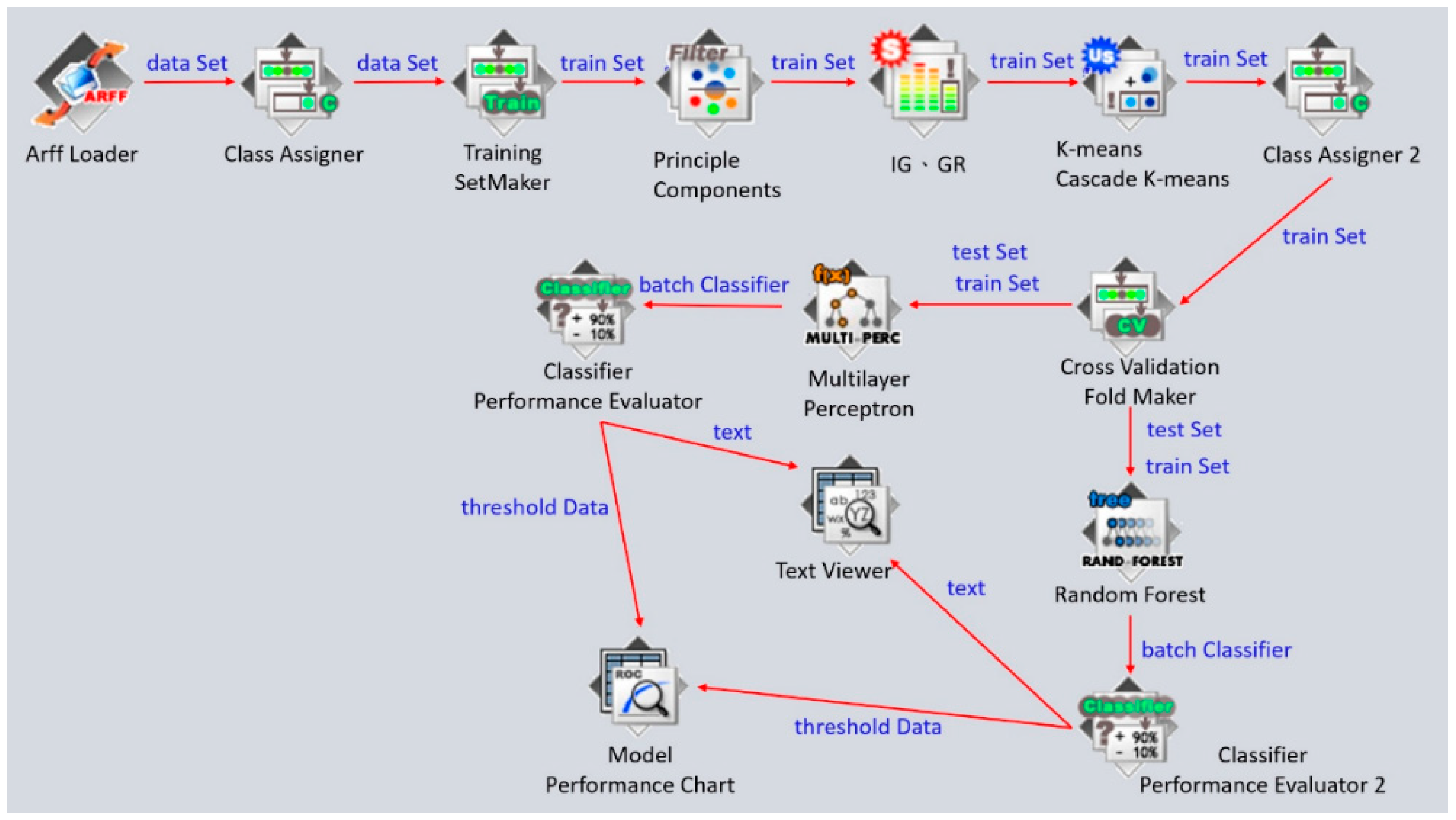
3.4.2. Clustering Analysis and Classification
4. Results
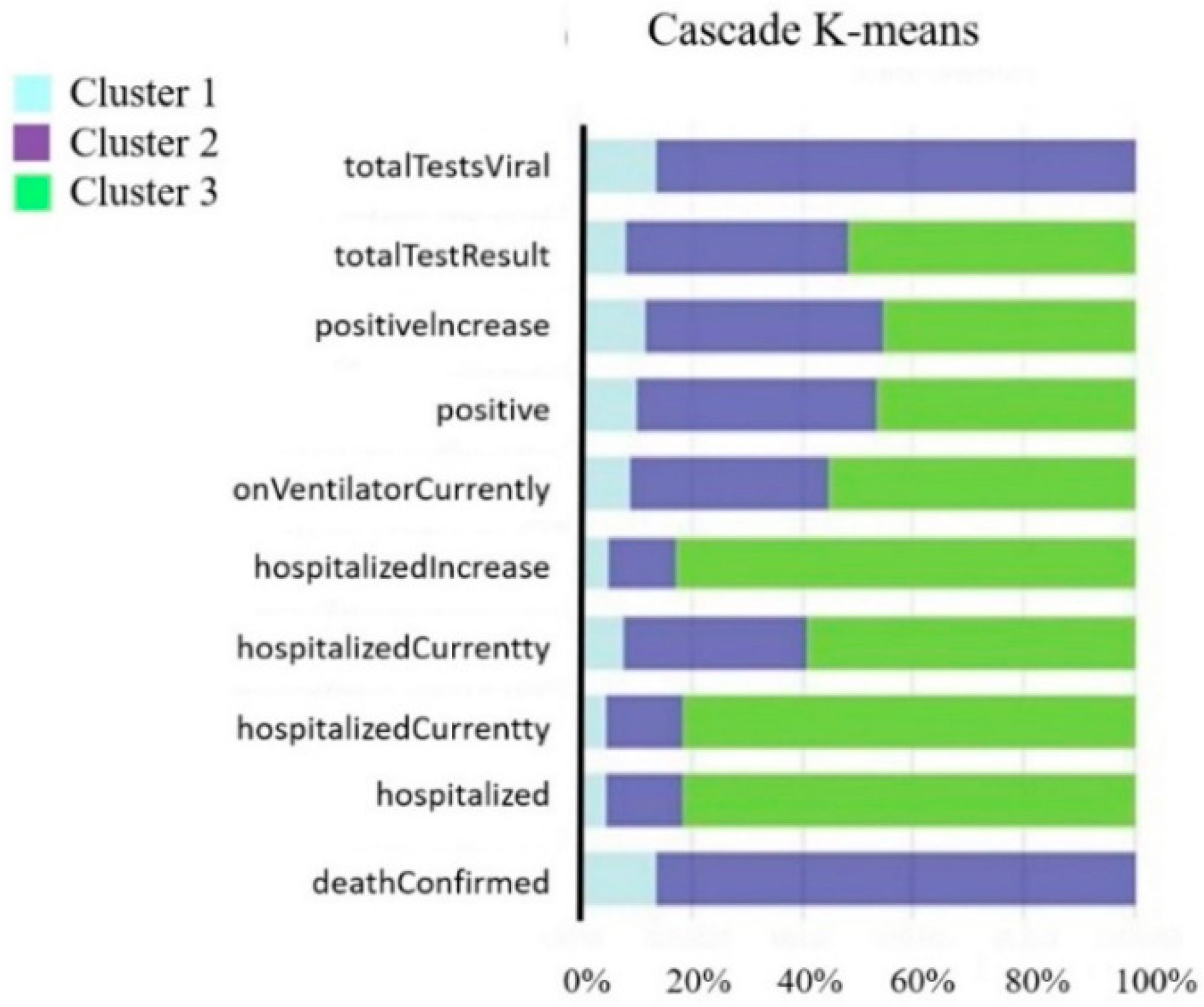
4.1. Feature Selection and Clustering Analysis Result
4.2. Classification Validation
4.2.1. Validation of Random Forest
4.2.2. Validation of Neural Network
5. Discussion
6. Conclusions
Author Contributions
Funding
Institutional Review Board Statement
Informed Consent Statement
Data Availability Statement
Conflicts of Interest
References
- CDC COVID-19 Response Team; Bialek, S.; Boundy, E.; Bowen, V.; Chow, N.; Cohn, A.; Dowling, N.; Ellington, S.; Gierke, R.; Hall, A.; et al. Severe outcomes among patients with coronavirus disease 2019 (COVID-19)—United States, 12 February–16 March 2020. Morb. Mortal. Wkly. Rep. 2020, 69, 343–346. [Google Scholar]
- Jit, M.; Jombart, T.; Nightingale, E.S.; Endo, A.; Abbott, S.; Edmunds, W.J. Estimating number of cases and spread of coronavirus disease (COVID-19) using critical care admissions, United Kingdom, February to March 2020. Eurosurveillance 2020, 25, 2000632. [Google Scholar] [CrossRef]
- Chen, S.I.; Wu, C.Y.; Wu, Y.H.; Hsieh, M.W. Optimizing influenza vaccine policies for controlling 2009-like pandemics and regular outbreaks. PeerJ 2019, 7, e6340. [Google Scholar] [CrossRef]
- Kurbucz, M.T. A joint dataset of official COVID-19 reports and the governance, trade and competitiveness indicators of World Bank group platforms. Data Brief 2020, 31, 105881. [Google Scholar] [CrossRef]
- Liu, T.; Gong, D.; Xiao, J.; Hu, J.; He, G.; Rong, Z.; Ma, W. Cluster infections play important roles in the rapid evolution of COVID-19 transmission: A systematic review. Int. J. Infect. Dis. 2020, 99, 374–380. [Google Scholar] [CrossRef] [PubMed]
- Álvarez, J.D.; Matias-Guiu, J.A.; Cabrera-Martín, M.N.; Risco-Martín, J.L.; Ayala, J.L. An application of machine learning with feature selection to improve diagnosis and classification of neurodegenerative disorders. BMC Bioinform. 2019, 20, 1–12. [Google Scholar] [CrossRef] [Green Version]
- Hasegawa, M.; Sakurai, D.; Higashijima, A.; Niiya, I.; Matsushima, K.; Hanada, K.; Kuroda, K. Towards automated gas leak detection through cluster analysis of mass spectrometer data. Fusion Eng. Des. 2022, 180, 113199. [Google Scholar] [CrossRef]
- Trelohan, M.; François-Lecompte, A.; Gentric, M. Tourism development or nature protection? Lessons from a cluster analysis based on users of a French nature-based destination. J. Outdoor Recreat. Tour. 2022, 39, 100496. [Google Scholar] [CrossRef]
- Dzuba, S.; Krylov, D. Cluster analysis of financial strategies of companies. Mathematics 2021, 9, 3192. [Google Scholar] [CrossRef]
- Ghavidel, M.; Azhdari, S.M.H.; Khishe, M.; Kazemirad, M. Sonar data classification by using few-shot learning and concept extraction. Appl. Acoust. 2022, 195, 108856. [Google Scholar] [CrossRef]
- Tepe, C.; Demir, M.C. Real-Time Classification of EMG Myo Armband Data Using Support Vector Machine; IRBM: Pomezia, Italy, 2022. [Google Scholar]
- Dritsas, E.; Trigka, M. Stroke risk prediction with machine learning techniques. Sensors 2022, 22, 4670. [Google Scholar] [CrossRef]
- Huang, W.; Wu, Q.; Chen, Z.; Xiong, Z.; Wang, K.; Tian, J.; Zhang, S. The potential indicators for pulmonary fibrosis in survivors of severe COVID-19. J. Infect. 2021, 82, e5–e7. [Google Scholar] [CrossRef]
- Zhou, F.; Yu, T.; Du, R.; Fan, G.; Liu, Y.; Liu, Z.; Cao, B. Clinical course and risk factors for mortality of adult inpatients with COVID-19 in Wuhan, China: A retrospective cohort study. Lancet 2020, 395, 1054–1062. [Google Scholar] [CrossRef]
- Zheng, Z.; Peng, F.; Xu, B.; Zhao, J.; Liu, H.; Peng, J.; Tang, W. Risk factors of critical & mortal COVID-19 cases: A systematic literature review and meta-analysis. J. Infect. 2020, 81, e16–e25. [Google Scholar] [PubMed]
- Pan, T.; Fang, K. An effective information support system for medical management: Indicator based intelligence system. Int. J. Comput. Appl. 2010, 32, 119–124. [Google Scholar]
- Chang, S.J.; Hsiao, H.C.; Huang, L.H.; Chang, H. Taiwan quality indicator project and hospital productivity growth. Omega 2011, 39, 14–22. [Google Scholar] [CrossRef]
- Mainz, J.; Krog, B.R.; Bjørnshave, B.; Bartels, P. Nationwide continuous quality improvement using clinical indicators: The Danish National Indicator Project. Int. J. Qual. Health Care 2004, 16 (Suppl. 1), i45–i50. [Google Scholar] [CrossRef]
- Medlock, J.; Galvani, A.P. Optimizing influenza vaccine distribution. Science 2009, 325, 1705–1708. [Google Scholar] [CrossRef]
- Enayati, S.; Özaltın, O.Y. Optimal influenza vaccine distribution with equity. Eur. J. Oper. Res. 2020, 283, 714–725. [Google Scholar] [CrossRef]
- Abdi, H.; Williams, L.J. Principal component analysis. Wiley Interdiscip. Rev. Comput. Stat. 2010, 2, 433–459. [Google Scholar] [CrossRef]
- Ramesh, G.; Madhavi, K.; Reddy, P.D.K.; Somasekar, J.; Tan, J. Improving the accuracy of heart attack risk prediction based on information gain feature selection technique. Mater. Today Proc. 2022, in press. [Google Scholar] [CrossRef]
- Karegowda, A.G.; Manjunath, A.S.; Jayaram, M.A. Comparative study of attribute selection using gain ratio and correlation based feature selection. Int. J. Inf. Technol. Knowl. Manag. 2010, 2, 271–277. [Google Scholar]
- Na, S.; Xumin, L.; Yong, G. Research on k-means clustering algorithm: An improved k-means clustering algorithm. In Proceedings of the 2010 Third International Symposium on Intelligent Information Technology and Security Informatics, Jinggangshan, China, 2–4 April 2010; pp. 63–67. [Google Scholar]
- Desgraupes, B. Clustering indices. Univ. Paris Ouest-Lab Modal’X 2013, 1, 34. [Google Scholar]
- Shi, T.; Horvath, S. Unsupervised learning with random forest predictors. J. Comput. Graph. Stat. 2006, 15, 118–138. [Google Scholar] [CrossRef]
- Wang, S.C. Artificial neural network. In Interdisciplinary Computing in Java Programming; Springer: Boston, MA, USA, 2003; pp. 81–100. [Google Scholar]
- Murtagh, F.; Contreras, P. Algorithms for hierarchical clustering: An overview. Wiley Interdiscip. Rev. Data Min. Knowl. Discov. 2.1 2012, 2, 86–97. [Google Scholar] [CrossRef]
- Rani, Y.; Rohil, H. A study of hierarchical clustering algorithm. Int. J. Inf. Comput. Technol. 2013, 3, 1115–1122. [Google Scholar]
- Campello, R.J.; Kröger, P.; Sander, J.; Zimek, A. Density-based clustering. Wiley Interdiscip. Rev. Data Min. Knowl. Discov. 2020, 10, e1343. [Google Scholar] [CrossRef]
- Chen, Z.; Ji, H. Graph-based clustering for computational linguistics: A survey. In Proceedings of the TextGraphs-5-2010 Workshop on Graph-Based Methods for Natural Language Processing, Uppsala, Sweden, 16 July 2010; pp. 1–9. [Google Scholar]
- Somasekar, H.; Naveen, K. Text Categorization and graphical representation using Improved Markov Clustering. Int. J. 2018, 11, 107–116. [Google Scholar] [CrossRef]
- Kameshwaran, K.; Malarvizhi, K. Survey on clustering techniques in data mining. Int. J. Comput. Sci. Inf. Technol. 2014, 5, 2272–2276. [Google Scholar]
- Mitra, P.; Murthy, C.A.; Pal, S.K. Unsupervised feature selection using feature similarity. IEEE Trans. Pattern Anal. Mach. Intell. 2002, 24, 301–312. [Google Scholar] [CrossRef]
- Uğuz, H. A two-stage feature selection method for text categorization by using information gain, principal component analysis and genetic algorithm. Knowl-Based Syst. 2011, 24, 1024–1032. [Google Scholar] [CrossRef]
- Zekić-Sušac, M.; Has, A.; Knežević, M. Predicting energy cost of public buildings by artificial neural networks, CART, and random forest. Neurocomputing 2021, 439, 223–233. [Google Scholar] [CrossRef]
- Reilev, M.; Kristensen, K.B.; Pottegård, A.; Lund, L.C.; Hallas, J.; Ernst, M.T.; Thomsen, R.W. Characteristics and predictors of hospitalization and death in the first 11 122 cases with a positive RT-PCR test for SARS-CoV-2 in Denmark: A nationwide cohort. Int. J. Epidemiol. 2020, 49, 1468–1481. [Google Scholar] [CrossRef]
- Swift, M.D.; Sampathkumar, P.; Breeher, L.E.; Ting, H.H.; Virk, A. Mayo Clinic’s multidisciplinary approach to Covid-19 vaccine allocation and distribution. NEJM Catal. Innov. Care Deliv. 2021, 2, 1–9. [Google Scholar]
- Bertsimas, D.; Ivanhoe, J.; Jacquillat, A.; Li, M.; Previero, A.; Lami, O.S.; Bouardi, H.T. Optimizing vaccine allocation to combat the COVID-19 pandemic. medRxiv 2020. [Google Scholar] [CrossRef]
- Wingert, A.; Pillay, J.; Gates, M.; Guitard, S.; Rahman, S.; Beck, A.; Hartling, L. Risk factors for severity of COVID-19: A rapid review to inform vaccine prioritisation in Canada. BMJ Open 2021, 11, e044684. [Google Scholar] [CrossRef]


| Item | Variables | Attribute | Item | Variables | Attribute |
|---|---|---|---|---|---|
| 1 | date | String | 24 | inlcucumulative | Numerical |
| 2 | state | String | 25 | inlcuCurrently | Numerical |
| 3 | dataQualityGrade | String | 26 | onVentilatorCumulative | Numerical |
| 4 | positive | Numerical | 27 | onVentilatorCurrently | Numerical |
| 5 | positive Increase | Numerical | 28 | death | Numerical |
| 6 | probable Cases | Numerical | 29 | death Increase | Numerical |
| 7 | positiveScore | Numerical | 30 | death Probable | Numerical |
| 8 | positiveCasesViral | Numerical | 31 | death Confirmed | Numerical |
| 9 | positiveTestsViral | Numerical | 32 | recovered | Numerical |
| 10 | positiveTestsPeopleAntibody | Numerical | 33 | totaltestResults | Numerical |
| 11 | positiveTestsAntibody | Numerical | 34 | totalTestResultsIncrease | Numerical |
| 12 | positiveTestsPeopleAntigen | Numerical | 35 | totalTestsViral | Numerical |
| 13 | positiveTestsAntigen | Numerical | 36 | totalTestsViralIncrease | Numerical |
| 14 | negative | Numerical | 37 | totalTestsPeopleViral | Numerical |
| 15 | negativeTestsViral | Numerical | 38 | totalTestsPeopleViralIncrease | Numerical |
| 16 | negativeTestsPeopleAntibody | Numerical | 39 | totalTestEncountersViral | Numerical |
| 17 | negativeTestsAntibody | Numerical | 40 | totalTestEncountersViralIncrease | Numerical |
| 18 | negativeIncrease | Numerical | 41 | totalTestsAntigen | Numerical |
| 19 | Pending | Numerical | 42 | totalTestsPeopleAntigen | Numerical |
| 20 | hospitalized | Numerical | 43 | totalTestsAntibody | Numerical |
| 21 | hospitalized Increase | Numerical | 44 | totalTestsPeopleAntibody | Numerical |
| 22 | hospitalized Cumulative | Numerical | |||
| 23 | hospitalized Currently | Numerical |
| Category | Hierarchical | Density-Based | Graph-Based | Partitioning |
|---|---|---|---|---|
| Based on | Linkage methods | Density accessibility Density connectivity | Graph theory | Mean Centroid Mediod-Centriod |
| Type of Data | Numerical | Numerical | Mix data | Numerical |
| Pros | Easy to implement Good for small datasets | Found clusters of arbitrary shapes and sizes | Perform well with complex shapes of data | Easy to implement Robust and easier to understand |
| Cons | Fails on larger sets Hard to find the correct number of clusters | Doe not work well in high dimensionality data. | Can be costly to compute | Unable to handle noisy data and outliers |
| Data Field | Minimum | Maximum | Mean | Standard Deviation |
|---|---|---|---|---|
| Death | 3.563 | 20,146.993 | 3012.726 | 4063.720 |
| deathConfirmed | 0.000 | 11,873.819 | 1612.264 | 2564.015 |
| deathIncrease | 0.229 | 139.083 | 23.802 | 28.186 |
| deathProbable | 0.000 | 1557.983 | 116.001 | 241.290 |
| Hospitalized | 0.000 | 74,908.536 | 6795.447 | 12,375.868 |
| hospitalizedCumulative | 0.000 | 74,908.536 | 6795.447 | 12,375.868 |
| hospitalizedCurrently | 0.000 | 5706.697 | 1016.505 | 1178.133 |
| hospitalizedIncrease | −0.868 | 574.361 | 52.537 | 93.318 |
| inIcuCumulative | 0.000 | 4167.848 | 374.140 | 935.623 |
| inIcuCurrently | 0.000 | 1594.500 | 198.782 | 310.440 |
| negative | 3193.583 | 5,676,868.213 | 1,217,574.982 | 1,393,361.630 |
| negativeIncrease | 225.347 | 66,790.590 | 10,430.280 | 13,289.475 |
| negativeTestsAntibody | 0.000 | 274,785.535 | 9939.138 | 42,390.124 |
| negativeTestsPeopleAntibody | 0.000 | 307,446.436 | 9400.504 | 44,786.195 |
| negativeTestsViral | 0.000 | 5,069,123.190 | 376,163.876 | 913,586.361 |
| onVentilatorCumulative | 0.000 | 1210.757 | 44.743 | 189.114 |
| onVentilatorCurrently | 0.000 | 383.805 | 77.040 | 115.523 |
| positive | 290.354 | 689,808.865 | 126,025.819 | 137,216.541 |
| positiveCasesViral | 0.000 | 644,108.814 | 99,837.740 | 122,787.805 |
| positiveIncrease | 16.833 | 6633.789 | 1390.662 | 1405.567 |
| positiveScore | 0.000 | 0.000 | 0.000 | 0.000 |
| positiveTestsAntibody | 0.000 | 32,553.559 | 2128.500 | 6739.150 |
| positiveTestsAntigen | 0.000 | 28,745.608 | 1748.258 | 5172.510 |
| positiveTestsPeopleAntibody | 0.000 | 30,843.331 | 969.265 | 4476.315 |
| positiveTestsPeopleAntigen | 0.000 | 19,372.812 | 912.666 | 3418.733 |
| positiveTestsViral | 0.000 | 746,688.084 | 69,991.507 | 149,301.079 |
| recovered | 0.000 | 548,376.917 | 56,375.980 | 91,104.014 |
| totalTestEncountersViral | 0.000 | 6,252,107.282 | 436,938.962 | 1,266,757.976 |
| totalTestEncountersViralIncrease | 0.000 | 70,634.798 | 4496.100 | 13,115.623 |
| totalTestResults | 3643.785 | 6,252,107.282 | 1,575,543.098 | 1,650,858.474 |
| totalTestResultsIncrease | 250.514 | 70,634.798 | 14,555.709 | 15,895.585 |
| totalTestsAntibody | 0.000 | 336,182.488 | 33,358.436 | 81,366.549 |
| totalTestsAntigen | 0.000 | 329,705.523 | 23,679.767 | 57,553.140 |
| totalTestsPeopleAntibody | 0.000 | 338,396.716 | 13,807.533 | 51,122.147 |
| totalTestsPeopleAntigen | 0.000 | 121,896.261 | 6203.051 | 21,180.165 |
| totalTestsPeopleViral | 0.000 | 3,939,157.669 | 424,758.638 | 718,630.307 |
| totalTestsPeopleViralIncrease | −251.653 | 31,530.365 | 3374.921 | 5665.766 |
| totalTestsViral | 0.000 | 5,972,478.403 | 1,244,215.985 | 1,591,549.099 |
| totalTestsViralIncrease | 0.000 | 52,143.061 | 11,304.525 | 14,366.747 |
| Features | |||||||||||
|---|---|---|---|---|---|---|---|---|---|---|---|
| Group | Pc1 | Pc2 | Pc3 | Pc4 | Pc5 | Pc6 | Pc7 | Pc8 | Pc9 | Pc10 | Pc11 |
| Variation | 15.89 | 6.05 | 4.69 | 2.64 | 1.90 | 1.38 | 1.11 | 0.92 | 0.64 | 0.54 | 0.49 |
| Variation Percentage | 0.42 | 0.16 | 0.12 | 0.07 | 0.05 | 0.04 | 0.03 | 0.02 | 0.02 | 0.01 | 0.01 |
| Cumulative contribution ratio | 0.42 | 0.58 | 0.70 | 0.77 | 0.82 | 0.85 | 0.88 | 0.91 | 0.93 | 0.94 | 0.96 |
| Rank | PCA | IG | GR | Average Rank |
|---|---|---|---|---|
| 1 | A30 | A2 | A39 | 2.7302 |
| 2 | A19 | A19 | A11 | 2.7302 |
| 3 | A21 | A30 | A13 | 2.7302 |
| 4 | A31 | A31 | A16 | 2.7302 |
| 5 | A8 | A13 | A18 | 2.7302 |
| 6 | A15 | A21 | A19 | 2.7302 |
| 7 | A24 | A12 | A38 | 2.7302 |
| 8 | A34 | A4 | A12 | 2.7302 |
| 9 | A14 | A8 | A9 | 2.7302 |
| 10 | A36 | A27 | A22 | 2.6814 |
| 11 | A9 | A38 | A8 | 2.4945 |
| 12 | A33 | A39 | A3 | 2.4945 |
| 13 | A6 | A20 | A4 | 2.4945 |
| 14 | A7 | A7 | A5 | 2.3984 |
| 15 | A23 | A6 | A6 | 2.3984 |
| 16 | A3 | A11 | A7 | 2.3269 |
| 17 | A5 | A9 | A21 | 2.3269 |
| 18 | A39 | A36 | A20 | 2.2745 |
| 19 | A29 | A18 | A2 | 1.9183 |
| 20 | A18 | A3 | A31 | 1.9183 |
| Code | Variable | Definition |
|---|---|---|
| A3 | deathConfirmed | Number of confirmed deaths |
| A6 | Hospitalized | Number of hospitalizations |
| A7 | hospitalizedCumulative | Cumulative hospitalizations |
| A8 | hospitalizedCurrently | Number of people currently hospitalized |
| A9 | hospitalizedIncrease | New hospitalizations |
| A18 | onVentilatorCurrently | Number of respirators currently in use |
| A19 | positive | Number of confirmed cases |
| A21 | positiveIncrease | The number of new diagnoses |
| A31 | totalTestResults | Total number of tests |
| A39 | totalTestsViralIncrease | Number of new PCR tests |
| Method | FS + K-Means Clustering | FS + Cascade K-Means Clustering | ||||
|---|---|---|---|---|---|---|
| Group | Cluster1 | Cluster2 | Cluster3 | Cluster3 | Cluster1 | Cluster2 |
| Count | 5 states | 5 states | 41 states | 7 states | 22 states | 22 states |
| cluster member | LA MO NC PA TN | IL MA MI OH TX | AK, AL, AR, AZ, CO, CT, DC, DE, FL, GA, GU, HI, IA, ID, IN, KS, KY, MD, ME, MN, MS, MT, ND, NE, NH, NJ, NM, NV, NY, OK, OR, PR, RI, SC, SD, UT, VA, VT, WA, WI, WY | IL LA MI MO NC PA TX | AL, AR, AZ, CO, FL, GA, IN, KY, MA, MD, MN, MS, NJ, NM, NY, OH, OK, SC, TN, UT, VA, WI | AK, CT, DC, DE, GU, HI, IA, ID, KS, ME, MT, ND, NE, NH, NV, OR, PR, RI, SD, VT, WA, WY |
| Source | Sum of Squares | df | p-Value |
|---|---|---|---|
| deathConfirmed | 96,309,899.004 | 2 | 0.000 *** |
| hospitalized | 163,810,675.372 | 2 | 0.595 |
| hospitalizedCumulative | 163,810,675.372 | 2 | 0.595 |
| hospitalizedCurrently | 20,454,751.196 | 2 | 0.000 *** |
| hospitalizedIncrease | 10,452.301 | 2 | 0.558 |
| onVentilatorCurrently | 171,650.041 | 2 | 0.001 *** |
| positive | 297,933,527,997.266 | 2 | 0.000 *** |
| positiveIncrease | 33,214,641.966 | 2 | 0.000 *** |
| totalTestResults | 56,194,090,472,628.98 | 2 | 0.000 *** |
| totalTestsViral | 73,640,463,254,532.75 | 2 | 0.000 *** |
| Source | Sum of Squares | df | p-Value |
|---|---|---|---|
| deathConfirmed | 92,467,765.941 | 2 | 0.000 *** |
| hospitalized | 2,542,735,930.524 | 2 | 0.000 *** |
| hospitalizedCumulative | 2,542,735,930.524 | 2 | 0.000 *** |
| hospitalizedCurrently | 28,731,039.605 | 2 | 0.000 *** |
| hospitalizedIncrease | 146,195.267 | 2 | 0.000 *** |
| onVentilatorCurrently | 182,801.937 | 2 | 0.000 *** |
| positive | 428,233,021,802.748 | 2 | 0.000 *** |
| positiveIncrease | 47,433,754.861 | 2 | 0.000 *** |
| totalTestResults | 62,516,522,292,791.39 | 2 | 0.000 *** |
| totalTestsViral | 53,777,136,225,256.51 | 2 | 0.000 *** |
| Confusion Matrix | Clustering Class | ||||
|---|---|---|---|---|---|
| Cluster1 | Cluster2 | Cluster3 | |||
| a | b | c | |||
| Prediction Class | Cluster1 | a | 0 | 5 | |
| Cluster2 | b | 0 | 4 | ||
| Cluster3 | c | 0 | 0 | ||
| Confusion Matrix | Clustering Class | ||||
|---|---|---|---|---|---|
| Cluster1 | Cluster2 | Cluster3 | |||
| a | b | c | |||
| Prediction Class | Cluster1 | a | 1 | 0 | |
| Cluster2 | b | 0 | 0 | ||
| Cluster3 | c | 0 | 0 | ||
| Confusion Matrix | Clustering Class | ||||
|---|---|---|---|---|---|
| Cluster1 | Cluster2 | Cluster3 | |||
| a | b | c | |||
| Prediction Class | Cluster1 | a | 0 | 5 | |
| Cluster2 | b | 2 | 1 | ||
| Cluster3 | c | 0 | 2 | ||
| Confusion Matrix | Clustering Class | ||||
|---|---|---|---|---|---|
| Cluster1 | Cluster2 | Cluster3 | |||
| a | b | c | |||
| Prediction Class | Cluster1 | a | 3 | 0 | |
| Cluster2 | b | 0 | 0 | ||
| Cluster3 | c | 3 | 0 | ||
| Clustering | K-Means | Cascade K-Means | ||
|---|---|---|---|---|
| Validation | RF | NN | RF | NN |
| Accuracy | 0.8235 | 0.8039 | 0.9803 | 0.8823 |
| Precision | 1 | 0.911 | 1 | 0.938 |
| Recall | 0.824 | 0.872 | 0.98 | 0.938 |
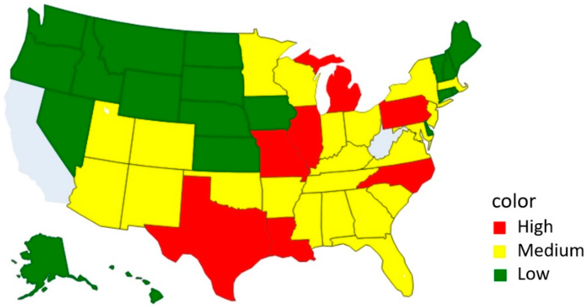
| Severity | States |
|---|---|
| Low | AK, CT, DC, DE, GU, HI, IA, ID, KS, ME, MT, ND, NE, NH, NV, OR, PR, RI, SD, VT, WA, WY |
| Medium | AL, AR, AZ, CO, FL, GA, IN, KY, MA, MD, MN, MS, NJ, NM, NY, OH, OK, SC, TN, UT, VA, WI |
| High | IL, LA, MI, MO, NC, PA, TX |
Publisher’s Note: MDPI stays neutral with regard to jurisdictional claims in published maps and institutional affiliations. |
© 2022 by the authors. Licensee MDPI, Basel, Switzerland. This article is an open access article distributed under the terms and conditions of the Creative Commons Attribution (CC BY) license (https://creativecommons.org/licenses/by/4.0/).
Share and Cite
Shih, D.-H.; Shih, P.-L.; Wu, T.-W.; Li, C.-J.; Shih, M.-H. Cluster Analysis of US COVID-19 Infected States for Vaccine Distribution. Healthcare 2022, 10, 1235. https://doi.org/10.3390/healthcare10071235
Shih D-H, Shih P-L, Wu T-W, Li C-J, Shih M-H. Cluster Analysis of US COVID-19 Infected States for Vaccine Distribution. Healthcare. 2022; 10(7):1235. https://doi.org/10.3390/healthcare10071235
Chicago/Turabian StyleShih, Dong-Her, Pai-Ling Shih, Ting-Wei Wu, Cheng-Jung Li, and Ming-Hung Shih. 2022. "Cluster Analysis of US COVID-19 Infected States for Vaccine Distribution" Healthcare 10, no. 7: 1235. https://doi.org/10.3390/healthcare10071235
APA StyleShih, D.-H., Shih, P.-L., Wu, T.-W., Li, C.-J., & Shih, M.-H. (2022). Cluster Analysis of US COVID-19 Infected States for Vaccine Distribution. Healthcare, 10(7), 1235. https://doi.org/10.3390/healthcare10071235