Analysis of Time-Delay Epidemic Model in Rechargeable Wireless Sensor Networks

Abstract

With the development of wireless rechargeable sensor networks (WRSNs), many scholars began to attach attention to network security under the spread of viruses. This paper mainly studies a novel low-energy-status-based model SISL (Susceptible, Infected, Susceptible, Low-Energy). The conversion process from low-energy nodes to susceptible nodes is called charging. It is noted that the time delay of the charging process in WRSNs should be considered. However, the charging process and its time delay have not been investigated in traditional epidemic models in WRSNs. Thus, the model SISL is proposed. The basic reproduction number, the disease-free equilibrium point, and the endemic equilibrium point are discussed here. Meanwhile, local stability and global stability of the disease-free equilibrium point and the endemic equilibrium point are analyzed. The addition of the time-delay term needs to be analyzed to determine whether it affects the stability. The intervention treatment strategy under the optimal control is obtained through the establishment of the Hamiltonian function and the application of the Pontryagin principle. Finally, the theoretical results are verified by simulations.

1. Introduction

With the development of science and technology, the research of wireless sensor networks (WSNs) has attracted scholars’ attention in recent years. By organizing and combining sensor nodes freely through wireless communication technology, WSNs are established [1,2]. A WSN is a distributed sensor network, and its end is a sensor that can sense and check the outside environment. Sensors in WSNs communicate wirelessly, so the network setting is flexible, and the device position can be changed at any time. WSNs are widely applied in various fields such as military facilities, home automation, and the interconnection of transportation systems [3]. Wireless rechargeable sensor network (WRSN) technology came into being under the wireless power transfer (WPT) technology. Thus, the research of wireless sensors has been pushed to a new level.

However, WRSNs are usually vulnerable to malware attacks [4,5,6], such as denial of service, malicious code distribution, and information exfiltration [7]. WRSNs especially suffer from the Denial of Charge (DOC) [8]. It is of great significance to study the network security of WRSNs.

The security of sensor networks has become a hot research field [9,10]. The research methods here are as follows:

• Establish a mathematical epidemics model.
• Analyze the equilibrium point in the system, and study its stability.
• Achieve the optimal control to make the control of malware propagation more effective. According to previous studies, the classical mathematical models established by predecessors mainly include the following: SIS (Susceptible, Infected, Susceptible), SIR (Susceptible, Infected, Removed), and SIRS (Susceptible, Infected, Removed, Susceptible).

There is a class of nodes called low-energy nodes (L) in wireless rechargeable sensor networks. In the traditional research of wireless sensor network security, the migration process from low-energy nodes (L) to operational nodes (S or I) is seldom considered. Since the SILS (Susceptible, Infected, Low-energy, Susceptible) model was put forward in 2021 [11], we began to pay attention to the research on the influence of low-energy nodes. What is particularly emphasized in the SILS model is the influence of the charging process on system safety control. What is more, charging will inevitably bring about a time delay in WRSNs. Thus, the SILS model [11] is modified by adding the time-delay term in this paper, to study the influence of time delay on WRSNs.

Table 1. Related research on epidemic models under time delay.

Authors	Model	Characteristics	Bifurcation	Enhancements
Zhu, L. et al. [12]	SBD (Susceptible-Believed-Denied)	Time delay of the rumor spreading	1	Establishment and analysis of SBD rumor-spreading model.
Zhu, L. et al. [13]	SIRS (Susceptible-Infected-Recovered-Susceptible)	Time delay of the immune validity	2	Consideration of immune validity period and the analysis of the optimal control.
Zhang, Z. et al. [14]	SEIRS-V (Susceptible-Exposed-Infected-Recovered-Susceptible and Vaccinated)	Time delay of the immune validity; the recovery and the vaccination	2	Introduction of the vaccinated nodes and the analysis of double time delays.
Liu, J. et al. [15]	SEIR (Susceptible-Exposed-Infected-Recovered)	Time delay of the exposure	2	Consideration of infectious-disease models with different incubation periods.
Wang, C. et al. [16]	SEIRS (Susceptible-Exposed-Infected-Recovered-Susceptible)	Time delay of the exposure and the immune validity	2	Consideration of immune validity period and the analysis of double time delays.
Zhang, Z. et al. [17]	SEIRS-V (Susceptible-Exposed-Infected-Recovered-Susceptible and Vaccinated)	Time delay of the immunity and the immune validity	2	Introduction of the vaccinated nodes and the analysis of double time delays.
Zhu, L. et al. [18]	SIS (Susceptible-Infected-Susceptible)	Time delay of the incubation	2	Time-delay analysis of recovery process based on SIS model.
Zhang, Z. et al. [19]	SEIQRS-V (Susceptible-Exposed-Infected-Quarantined -Recovered-Susceptible and Vaccinated)	Time delay of the exposure	2	Infectious-disease model considering the nodes’ distribution area.
Zhu, L. et al. [20]	SEIR (Susceptible-Exposed-Infected-Recovered)	Time delay of the incubation	1	Time-delay analysis of infection process based on SEIR system.
Al-Darabsah, I. et al. [21]	SEIRS-V (Susceptible-Exposed-Infected-Recovered-Susceptible and Vaccinated)	Time delay of the exposure	1	Time-delay analysis considering specific effective contact rate.

1: Hopf bifurcation does not occur under the change of time delay. 2: Hopf bifurcation occurs as the time delay increases to a certain value.

shows that predecessors have done much work on time-delay research. A time delay occurs in the migration behavior of different nodes in epidemic or rumor models. It is necessary to investigate the stability problem under time delay and Hopf bifurcation [12,13,14,15,16,17,18,19,20,21]. It is noted that time delay not only affects the convergence but also affects the control strategy in different models. Thus, the time-delay-based methods under the Pontryagin’s minimum principle are adapted to study the optimal control [22].

However, we know that the time delay of the charging process in WRSNs has not been investigated previously. This paper mainly provides a kind of influence on time delay based on the SIS model combined with low-energy nodes (L) [23,24,25]. Thus, a novel epidemic model (1) of virus spreading in WRSNs is developed.

The virus-propagation rules and the optimal control strategy of the model (1) is proposed as follows:

• A novel low-energy-status-based model is introduced to describe the propagation process of malicious software (virus) in WRSNs.
• The basic reproduction number is defined by the disease-free equilibrium solution and the epidemic equilibrium solution. The Routh criterion is applied to prove the local stability, and the Lyapunov universal function is constructed to prove the global attraction.
• Based on Pontryagin’s minimum principle, the optimal control variables satisfying the minimization of the objective function are obtained.
• The stability problem under time delay is specially revealed.

The rest of the paper is as follows: the introduction and analysis of the model are presented in Section 2; the dynamic stability analysis is given in Section 3; the optimal control theory is presented in Section 4; the analysis of the influence of time delay is given in Section 5;. the simulation results are given in Section 6; and the conclusions are summarized in Section 7.

2. Modeling Analysis

As mentioned above, a classical model called SIS can be applied in wireless sensor networks. However, the SIS model can be modified by increasing the low-energy status L(t) in WRSNs [11]. The modified model here is shown in Figure 1. Different from the model in [11], in order to control malware more efficiently, charging low-energy-infected nodes is neglected. The process of the nodes L(t) converting into S(t) is called charging. The feature of the charging process is its latency. First, without considering the time delay, the system (1) is discussed here (with the initial values $\left(0\right)={\Phi }_S, I\left(0\right)={\Phi }_I, L\left(0\right)=0, D\left(0\right)=0, 0\le {\Phi }_{S,I}\le \frac{\wedge }{d}$). Parameters are shown in

Table 2. Significance of the model parameters.

S(t)	The quantity of the susceptible node
I(t)	The quantity of the infected node
L(t)	The quantity of the low-energy node
∧	Injection rate of system
α1	Transmission rate of malware
α2	Self-disinfection rate of the infected nodes
c	Charging success rate
μ	Low-energy-node conversion rate
d	Node deactivation rate

.

$$\{\begin{array}{c}\frac{dS(t)}{dt}=\wedge -{\alpha }_{1}S(t)I(t)+{\alpha }_{2}I(t)-dS(t)+cL(t)-\mu S(t)\\ \frac{dI(t)}{dt}={\alpha }_{1}S(t)I(t)-{\alpha }_{2}I(t)-dI(t)-\mu I(t)\\ \frac{dL(t)}{dt}=-dL(t)-cL(t)+\mu S(t)\\ \frac{dD(t)}{dt}=dL(t)+dS(t)+dI(t)+\mu I(t)\end{array}$$

(1)

In order to further study the dynamic balance of the system, and the propagation law of malicious programs, the equilibrium solution of the system needs to be found first. By studying the stability and transformation behavior of each equilibrium solution, the general law of malware control could be drawn, and intervention for controlling the spreading of malicious programs could be easily put forward.

From the numerical relationship, the system (1) has two equilibrium solutions (the disease-free equilibrium solution $E_0$ and the endemic equilibrium solution $E_{+}$). The solutions $E_0$ and $E_{+}$ are depicted as follows:

$$E_0\left(S_0,I_0,L_0\right)=\left(\frac{\wedge \left(d+c\right)}{\left(d+\mu \right)\left(d+c\right)-c\mu } , 0 , \frac{\mu \wedge }{\left(d+\mu \right)\left(d+c\right)-c\mu }\right);$$

(2)

$$E_{+}\left(S_{+},I_{+},L_{+}\right)=\left(\frac{{\alpha }_2+d+\mu }{{\alpha }_1} , \frac{ \wedge -\frac{{\alpha }_2{d}^2+d^3+\mu d^2+{\alpha }_2\mu d+\mu d^2+{\mu }^{2}d+{\alpha }_{2}dc+d^{2}c+\mu dc}{{\alpha }_1\left(d+c\right)} }{d+\mu } , \frac{\mu ({\alpha }_2+d+\mu )}{{\alpha }_1\left(d+c\right)}\right)$$

(3)

The basic reproduction number $R_0$ is given as

$$R_0=\frac{S_0}{S_{+}}=\frac{\wedge \left(d+c\right){\alpha }_1}{\left[\left(d+\mu \right)\left(d+c\right)-c\mu \right]\left({\alpha }_2+d+\mu \right)}.$$

(4)

If $\left(d+\mu \right)\left(d+c\right)-c\mu >0$, we can put forth the following theorem:

Theorem 1.

If$R_0<1$, the system only has a unique disease-free equilibrium solution$E_0$. While$R_0\ge 1$, the system (1) has an endemic equilibrium solution$E_{+}$and a disease-free equilibrium solution$E_0$.

3. Dynamic-Stability Analysis

In this section, we focus on analyzing the local stability of the system (1) by using the linearization technique and the Routh–Herwitz criterion. However, the global stability is analyzed by constructing a Lyapunov universal function.

3.1. Local Stability Analysis

Theorem 2.

If$R_0<1$,the disease-free equilibrium point$E_0$is locally stable.

Proof. 

First of all, the system is linearized as follows:

$$\{\begin{array}{c}\frac{dS\left(t\right)}{dt}=J_{11}\left(S-S_{*}\right)+J_{12}\left(I-I_{*}\right)+J_{13}\left(L-L_{*}\right)\\ \frac{ dI\left(t\right)}{dt}=J_{21}\left(S-S_{*}\right)+J_{22}\left(I-I_{*}\right)+J_{23}\left(L-L_{*}\right)\\ \frac{ dL\left(t\right)}{dt}=J_{31}\left(S-S_{*}\right)+J_{32}\left(I-I_{*}\right)+J_{33}\left(L-L_{*}\right)\end{array}$$

(5)

$$J\left(E_{*}\right)=\left(\begin{array}{ccc}{J}_{11}& J_{12}& J_{13}\\ J_{21}& J_{22}& J_{23}\\ J_{31}& J_{32}& J_{33}\end{array}\right)=\left(\begin{array}{ccc}-{\alpha }_{1}I-d-\mu & -{\alpha }_{1}S+{\alpha }_2& c\\ {\alpha }_{1}I& {\alpha }_{1}S-{\alpha }_2-d-\mu & 0\\ \mu & 0& -d-c\end{array}\right)$$

(6)

$J\left(E_{*}\right)$ is the corresponding Jacobian matrix, in which “*” represents “0” or “+”. The characteristic equation is constructed using Formula (6):

$$\left|\lambda I-J\left(E_0\right)\right|=\left|\begin{array}{ccc}\lambda +d+\mu & {\alpha }_1{S}_0-{\alpha }_2& -c\\ 0& \lambda -{\alpha }_1{S}_0+{\alpha }_2+d+\mu & 0\\ -\mu & 0& \lambda +d+c\end{array}\right|=0$$

(7)

which gives the following equation:

$$\begin{array}{c}\left(\lambda +d+\mu \right)\left(\lambda -{\alpha }_1{S}_0+{\alpha }_2+d+\mu \right)\left(\lambda +d+c\right)-c\mu \left(\lambda -{\alpha }_1{S}_0+{\alpha }_2+d+\mu \right)\\ =\left[\left(\lambda +d+\mu \right)\left(\lambda +d+c\right)-c\mu \right]\left(\lambda -{\alpha }_1{S}_0+{\alpha }_2+d+\mu \right)\\ =\left(\lambda +d\right)\left(\lambda +d+\mu +c\right)\left[\lambda -\left({\alpha }_2+d+\mu \right)\left(R_0-1\right)\right]=0\end{array}$$

(8)

Thus, if $R_0<1,$

$$\begin{array}{c}{\lambda }_1=-d;\\ {\lambda }_2=-d-\mu -c;\\ {\lambda }_3=\left({\alpha }_2+d+\mu \right)\left(R_0-1\right)<0.\end{array}$$

(9)

Theorem 2 is valid under the theory of the Hurwitz criterion. □

Theorem 3.

If$R_0\ge 1$, the endemic equilibrium point$E_{+}$is locally stable.

Proof. 

The analysis method is the same as above. The characteristic equation of $J\left(E_{+}\right)$ is found as follows:

$$\begin{array}{cc}\left|\lambda I-J(E_{+})\right|& = \left|\begin{array}{ccc}\lambda +{\alpha }_1{I}_{+}+d+\mu & {\alpha }_1{S}_{+}-{\alpha }_2& -c\\ -{\alpha }_1{I}_{+}& \lambda -{\alpha }_1{S}_{+}+{\alpha }_2+d+\mu & 0\\ -\mu & 0& \lambda +d+c\end{array}\right|\\ & = \left|\begin{array}{ccc}\lambda +{\alpha }_1{I}_{+}+d+\mu -{\alpha }_1{S}_{+}+{\alpha }_2& {\alpha }_1{S}_{+}-{\alpha }_2& -c\\ 0& \lambda +d+\mu & -c\\ -\mu & 0& \lambda +d+c\end{array}\right|\\ & = 0,\end{array}$$

(10)

which donates the following equation:

$$\begin{array}{c}\left(\lambda -{\alpha }_1{I}_{+}+d+\mu -{\alpha }_1{S}_{+}+{\alpha }_2\right)\left(\lambda +d+\mu \right)\left(\lambda +d+c\right)+\left({\alpha }_1{S}_{+}-{\alpha }_2\right)c\mu -c\mu \left(\lambda +d+\mu \right)\\ ={\lambda }^3+\left(\frac{{\alpha }_1\wedge \left(R_0-1\right)}{R_0\left(d+\mu \right)}+d+\mu +c+d\right){\lambda }^2\\ +\left[\frac{d{\alpha }_1\wedge \left(R_0-1\right)}{R_0\left(d+\mu \right)}+\left(d+\mu +c\right)\left(\frac{{\alpha }_1\wedge \left(R_0-1\right)}{R_0\left(d+\mu \right)}\right)+\left(d+\mu +c\right)d\right]\\ +\left[\frac{\left(d+\mu +c\right)d{\alpha }_1\wedge \left(R_0-1\right)}{R_0\left(d+\mu \right)}+\frac{{\alpha }_1\wedge \left(R_0-1\right)c\mu }{R_0\left(d+\mu \right)}\right]\\ =0.\end{array}$$

(11)

Set:

$$\{\begin{array}{c}{a}_3=1;\\ a_2=\left(\frac{{\alpha }_1\wedge (R_0-1)}{R_0(d+\mu )}+d+\mu +c+d\right)>0;\\ a_1=\left[\frac{d{\alpha }_1\wedge (R_0-1)}{R_0(d+\mu )}+(d+\mu +c)\left(\frac{{\alpha }_1\wedge (R_0-1)}{R_0(d+\mu )}\right)+(d+\mu +c)d\right]>0;\\ a_0=\frac{(d+\mu +c)d{\alpha }_1\wedge (R_0-1)}{R_0(d+\mu )}+\frac{{\alpha }_1\wedge (R_0-1)c\mu }{R_0(d+\mu )}>0.\end{array}$$

(12)

The following results could be obtained:

$$\{\begin{array}{cc}{\Delta }_1& = a_2>0\\ {\Delta }_2& = \left|\begin{array}{cc}{a}_2& a_0\\ a_3& a_1\end{array}\right|=\left(\frac{{\alpha }_1\wedge (R_0-1)}{R_0(d+\mu )}+d\right)\\ & \ast \left(d\frac{{\alpha }_1\wedge (R_0-1)}{R_0(d+\mu )}+(d+\mu +c)\frac{{\alpha }_1\wedge (R_0-1)}{R_0(d+\mu )}+(d+\mu +c)d\right)\\ & +(d+c)\left[(d+\mu )\left(\frac{{\alpha }_1\wedge (R_0-1)}{R_0(d+\mu )}+d\right)+c\frac{{\alpha }_1\wedge (R_0-1)}{R_0(d+\mu )}+cd\right]\\ & +\mu \left[(d+\mu )\left(\frac{{\alpha }_1\wedge (R_0-1)}{R_0(d+\mu )}+d\right)+cd\right]\\ & >0;\\ {\Delta }_3& = \left|\begin{array}{ccc}{a}_2& a_0& 0\\ a_3& a_1& 0\\ 0& a_2& a_0\end{array}\right|=a_0{\Delta }_2>0\end{array}$$

(13)

Theorem 3 is proved under the theory of the Hurwitz criterion. □

3.2. Global-Stability Analysis

In this section, we discuss the global stability by constructing a suitable Lyapunov universal function, which is positive definite except for the stable point.

Theorem 4.

If$R_0<1$,the disease-free equilibrium point$E_0$is globally asymptotically stable.

Proof. 

The Lyapunov function is defined as follows:

$$V_{E_0}\left(t\right)=\frac{1}{2}{\left(S-S_0\right)}^2+\frac{d+\mu }{{\alpha }_1}I+\frac{1}{2}{\left(L-L_0\right)}^2$$

(14)

If “t” tends to infinity, the disease-free equilibrium solution satisfies the following condition: $S\le S_0$.

Thus:

$$\begin{array}{cc}{V}_{E_0}^{\prime }\left(t\right)& =\left(S-S_0\right)\frac{dS}{dt}+\frac{d+\mu }{{\alpha }_1}\frac{dI}{dt}+\left(L-L_0\right)\frac{dL}{dt}\\ & =\left(S-S_0\right)\left[-{\alpha }_{1}SI+{\alpha }_1{S}_{0}I-{\alpha }_1{S}_{0}I+{\alpha }_{2}I-\left(d+\mu \right)\left(S-S_0\right)+c\left(L-L_0\right)\right]\\ & +\frac{d+\mu }{{\alpha }_1}\left[{\alpha }_{1}SI-\left({\alpha }_2+d+\mu \right)I\right]+\left(L-L_0\right)\left[-\left(d+c\right)\left(L-L_0\right)+\mu \left(S-S_0\right)\right]\\ & =-\left(d+\mu +{\alpha }_{1}I\right){\left(S-S_0\right)}^2-{\alpha }_1{S}_{0}I\left(S-S_0\right)+{\alpha }_{2}I\left(S-S_0\right)+c\left(L-L_0\right)\left(S-S_0\right)\\ & +\frac{d+\mu }{{\alpha }_1}\left({\alpha }_2+d+\mu \right)\left(R_0-1\right)I+\left(d+\mu \right)\left(S-S_0\right)I-\left(d+c\right){\left(L-L_0\right)}^2+\mu \left(S-S_0\right)\left(L-L_0\right)\\ & \le -\left(d+\frac{1}{2}\mu +{\alpha }_{1}I-\frac{1}{2}c\right){\left(S-S_0\right)}^2-\left({\alpha }_2+d+\mu \right)\left(R_0-1\right)I\left(S-S_0\right)\\ & +\frac{d+\mu }{{\alpha }_1}\left({\alpha }_2+d+\mu \right)\left(R_0-1\right)I -\left(d+\frac{1}{2}c-\frac{1}{2}\mu \right){\left(L-L_0\right)}^2\end{array}$$

(15)

Equation (15) shows $V_{E_0}^{\prime }\left(t\right)\le 0,if\left|\mu -c\right|\le 2dand{R}_0\le 1$.

What is more, $V_{E_0}\left(t\right)=0$ and $V_{E_0}^{\prime }\left(t\right)=0$ if and only if $S=S_0$ and $I=0$. Thus, Theorem 4 is valid. □

Theorem 5.

If$R_0\ge 1$, the endemic equilibrium point$E_{+}$is globally asymptotically stable.

Proof. 

Considering the conditions:

$$\{\begin{array}{c}0=\wedge -{\alpha }_1{S}_{+}{I}_{+}+{\alpha }_2{I}_{+}-d{S}_{+}+c{L}_{+}-\mu S_{+};\\ 0={\alpha }_1{S}_{+}{I}_{+}-{\alpha }_2{I}_{+}-d{I}_{+}-\mu I_{+};\\ 0=-d{L}_{+}-c{L}_{+}+\mu S_{+}\end{array}$$

(16)

the Lyapunov function is defined as follows:

$$V_{E_{+}}\left(t\right)=\frac{1}{2}{\left(S-S_{+}\right)}^2+\frac{d+\mu }{{\alpha }_1}\left(I-I_{+}+I_{+}ln\frac{I}{I_{+}}\right)+\frac{1}{2}{\left(L-L_{+}\right)}^2.$$

(17)

Thus:

$$\begin{array}{cc}{V}_{E_{+}}^{\prime }\left(t\right)& =\left(S-S_{+}\right)\frac{dS}{dt}+\frac{\left(d+\mu \right)}{{\alpha }_1}\frac{\left(I-I_{+}\right)}{I}\frac{dI}{dt}+\left(L-L_{+}\right)\frac{dL}{dt}\\ & =\left(S-S_{+}\right)\left[-{\alpha }_{1}SI+{\alpha }_1{S}_{+}{I}_{+}+{\alpha }_1{S}_{+}I-{\alpha }_1{S}_{+}I+{\alpha }_2\left(I-I_{+}\right)-\left(d+\mu \right)\left(S-S_{+}\right)+c\left(L-L_{+}\right)\right]\\ & +\frac{\left(d+\mu \right)}{{\alpha }_1}\frac{\left(I-I_{+}\right)}{I}\left[{\alpha }_{1}SI-{\alpha }_1{S}_{+}{I}_{+}+{\alpha }_1{S}_{+}I-{\alpha }_1{S}_{+}I-\left({\alpha }_2+d+\mu \right)\left(I-I_{+}\right)\right]\\ & +\left(L-L_{+}\right)\left[-\left(d+c\right)\left(L-L_{+}\right)+\mu \left(S-S_{+}\right)\right]\\ & =-\left(d+\mu +{\alpha }_{1}I\right){\left(S-S_{+}\right)}^2-\left(d+\mu \right)\left(I-I_{+}\right)\left(S-S_{+}\right)+c\left(L-L_{+}\right)\left(S-S_{+}\right)\\ & +\left(d+\mu \right)\left(S-S_{+}\right)\left(I-I_{+}\right)-\left(d+c\right){\left(L-L_{+}\right)}^2+\mu \left(S-S_{+}\right)\left(L-L_{+}\right)\\ & \le -\left(d+\frac{1}{2}\mu +{\alpha }_{1}I-\frac{1}{2}c\right){\left(S-S_{+}\right)}^2-\left(d+\frac{1}{2}c-\frac{1}{2}\mu \right){\left(L-L_{+}\right)}^2\end{array}$$

(18)

Equation (18) shows $V_{E_{+}}^{\prime }\left(t\right)\le 0,if\left|\mu -c\right|\le 2d$.

It is noted that $V_{E_{+}}\left(t\right)=0$ and $V_{E_{+}}^{\prime }\left(t\right)=0$ if and only if $S=S_{+}, I=I_{+}$ and $L=L_{+}$. Thus, Theorem 5 is confirmed. This means that the spread of malware will continue to exist in the system (1). □

4. Optimal-Control Analysis

In the practical application of malware control, intervention treatment is usually added to ensure that the spread of malware will not be epidemic. However, there is a certain cost due to intervention treatment. The Pontryagin minimum principle is adopted to solve the cost-minimization problem. Due to the characteristics of rechargeable systems, our optimization objectives are as follows: First, we must effectively control the spread of malware. The second objective is to ensure that the number of susceptible nodes in the system is not too small, and the low-energy nodes should be controlled within a certain number to ensure the normal operation of the system. Lastly, the cost of control needs to be feasible economically. Therefore, the system (1) is modified as follows (19):

$$\{\begin{array}{c}\frac{dS(t)}{dt}=\wedge -{\alpha }_{1}S(t)I(t)+{\alpha }_{2}I(t)-dS(t)+cL(t)-\mu S(t)+\mu (t)I(t)\\ \frac{dI(t)}{dt}={\alpha }_{1}S(t)I(t)-{\alpha }_{2}I(t)-dI(t)-\mu I(t)-\mu (t)I(t)\\ \frac{dL(t)}{dt}=-dL(t)-cL(t)+\mu S(t)\\ \frac{dD(t)}{dt}=dL(t)+dS(t)+dI(t)+\mu I(t)\end{array}$$

(19)

We establish an objective function:

$$G\left(u\right)=\underset{u}{\mathit{min}}\{I\left(tf\right)+L\left(tf\right)+{{\displaystyle \int }}_0^{tf}\left[c_1{u}^2\left(t\right)I^2\left(t\right)\right]dt\}$$

(20)

where $c_1$ is the cost coefficient of implementing intervention control, which mainly comes from the identification and removal of malicious software.; and u(t) is the intervention ratio, which satisfies $0\le u\left(t\right)\le 1$; tf is the end time of intervention.

It is obvious that the number of low-energy nodes and infected nodes at tf should be as few as possible, and the economic cost should be as low as possible. The Pontryagin minimum principle is applied to find the optimal proportion of intervention. The corresponding Hamiltonian function is as follows:

$$\begin{array}{cc}H& =c_1{u}^2\left(t\right)I^2\left(t\right)+{\beta }_1\left(t\right)\left(\wedge -{\alpha }_{1}SI+{\alpha }_{2}I-\left(d+\mu \right)S+ cL+u\left(t\right)I\right)\\ & +{\beta }_2\left(t\right)\left[{\alpha }_{1}SI-\left({\alpha }_2+d+\mu +u\left(t\right)\right)I\right]\end{array}$$

(21)

in which ${\beta }_i\left(t\right) \left(i=1,2,3\right)$ are covariates. The differential equation of covariant is as follows:

$$\{\begin{array}{c}\frac{d{\beta }_1}{dt}=-\frac{\partial H}{\partial S}={\beta }_1({\alpha }_{1}I+d+\mu )-{\beta }_2{\alpha }_{1}I-\mu {\beta }_3\\ \frac{d{\beta }_2}{dt}=-\frac{\partial H}{\partial I}=-2c_1{u}^2\left(t\right)I\left(t\right)+{\beta }_1({\alpha }_{1}S-{\alpha }_2-u(t\left)\right)+{\beta }_2({\alpha }_2+d+\mu +u(t)-{\alpha }_{1}S)\\ \frac{d{\beta }_3}{dt}=-\frac{\partial H}{\partial L}=-c{\beta }_1+{\beta }_3(d+c)\end{array}$$

(22)

The terminal constraints of the co-state variables are as follows:

$$\begin{array}{c}{\beta }_1\left(tf\right)=0;\\ {\beta }_2\left(tf\right)=1; \\ {\beta }_3\left(tf\right)=1.\end{array}$$

(23)

The optimal strategies are established by:

$$\frac{\partial H}{\partial u\left(t\right)}=2c_{1}u\left(t\right)I^2+{\beta }_{1}I-{\beta }_{2}I=0.$$

(24)

Then, the optimization variable can be obtained:

$$u^{*}\left(t\right)=\mathit{min}\left\{\mathit{max}\left(0,\frac{{\beta }_2-{\beta }_1}{2c_{1}I}\right),1\right\}.$$

(25)

5. Time-Delay System Analysis

If the number of system nodes is relatively large, the phenomenon of charging delay cannot be ignored. The time-delay item (t − τ) is considered in this section. In order to better study the influence of time delay, we need to explore whether the delay term will affect the stability of the system. The system is established as follows:

$$\{\begin{array}{c}\frac{dS(t)}{dt}=\wedge -{\alpha }_{1}S(t)I(t)+{\alpha }_{2}I(t)-dS(t)+cL(t-\tau )-\mu S(t)\\ \frac{dI(t)}{dt}={\alpha }_{1}S(t)I(t)-{\alpha }_{2}I(t)-dI(t)-\mu I(t)\\ \frac{dL(t)}{dt}=-dL(t)-cL(t)+\mu S(t)\\ \frac{dD(t)}{dt}=dL(t)+dS(t)+dI(t)+\mu I(t)\end{array}$$

(26)

5.1. Local-Stability Analysis

In this section, the characteristic solutions of the transcendental equations are explored by the theories in [26].

Theorem 6.

If$R_0<1$,the local stability at$E_0$of the system (26) is consistent with the stability of the system (1).

Suppose that for the characteristic equation of the system (26) at $E_0$, it has a pure imaginary characteristic solution $i{\omega }_0$.

The characteristic equation at $E_0$ is:

$$\left|\lambda I-J(E_0)\right|=\left|\begin{array}{ccc}\lambda +d+\mu & {\alpha }_1{S}_0-{\alpha }_2& -c{e}^{-\lambda \tau }\\ 0& \lambda -{\alpha }_1{S}_0+{\alpha }_2+d+\mu & 0\\ -\mu & 0& \lambda +d+c\end{array}\right|=0$$

(27)

The following formula can be obtained:

$$\begin{array}{c}\left(\lambda +d+\mu \right)\left(\lambda -{\alpha }_1{S}_0+{\alpha }_2+d+\mu \right)\left(\lambda +d+c\right)-\mu c{e}^{-\lambda \tau }\left(\lambda -{\alpha }_1{S}_0+{\alpha }_2+d+\mu \right)\\ =\left(\lambda -{\alpha }_1{S}_0+{\alpha }_2+d+\mu \right)\left[\left(\lambda +d+\mu \right)\left(\lambda +d+c\right)-c\mu e^{-\lambda \tau }\right]\\ =0.\end{array}$$

(28)

The root $\lambda ={\alpha }_1{S}_0-{\alpha }_2-d-\mu =0$ is negative. We set

$f_1\left(\lambda \right)=\left(\lambda +d+\mu \right)\left(\lambda +d+c\right)-c\mu e^{-\lambda \tau }=0$. Then,

$$\begin{array}{cc}{f}_1\left(i{\omega }_0\right)& =-{\omega }_0^2+\left(2d+\mu +c\right)i{\omega }_0+\left(d^2+d\mu +cd+c\mu -c\mu e^{-i{\omega }_0\tau }\right)\\ & =-{\omega }_0^2+\left(2d+\mu +c\right)i{\omega }_0\\ & +\left[d^2+d\mu +cd+c\mu -c\mu \left(\mathit{cos}{\omega }_0\tau -i\mathit{sin}{\omega }_0\tau \right)\right]\\ & =0.\end{array}$$

(29)

Separate the real and imaginary parts of the Equation (29):

$$-{\omega }_0^2+d^2+d\mu +cd+c\mu =c\mu cos{\omega }_0\tau ;$$

(30)

$$\left(2d+\mu +c\right){\omega }_0=-c\mu \mathit{sin}{\omega }_0\tau .$$

(31)

Square and add the two Equations (30) and (31):

$$c^2{\mu }^2={\left(2d+\mu +c\right)}^2{\omega }_0^2+{\left({\omega }_0^2+d^2+d\mu +cd+c\mu \right)}^2.$$

(32)

Set:

$$\{\begin{array}{c}{d}^2+d\mu +cd+c\mu =Q_2;\\ 2d+\mu +c=Q_1;\\ c\mu =Q_0;\\ {\omega }_0^2=v_0>0.\end{array}$$

(33)

Then,

$$f_1\left(i{\omega }_0\right)=v_0^2+\left(Q_1^2-2Q_2\right)v_0+Q_2^2-Q_0^2.$$

(34)

We can conclude that:

$$\{\begin{array}{c}{Q}_1^2-2Q_2=2d^2+2d\mu +2cd+{\mu }^2+c^2>0;\\ Q_2^2-Q_0^2={\left(d^2+d\mu +cd\right)}^2+2c\mu \left(d^2+d\mu +cd\right)>0.\end{array}$$

(35)

It can be obtained that Hypothesis 1 is not valid. Thus, Theorem 6 is proved.

Theorem 7.

If$R_0\ge 1$,the local stability at$E_{+}$of the system (26) is consistent with the stability of the system (1).

Suppose that for the characteristic equation of the system (26) at $E_{+}$, it has a pure imaginary characteristic solution $i{\omega }_0$.

For $E_{+}$, the solution is the same. Its characteristic equation at $E_{+}$ is:

$$\left|\lambda I-J\left(E_{+}\right)\right|=\left|\begin{array}{ccc}\lambda +d+\mu & {\alpha }_1{S}_0-{\alpha }_2& -c{e}^{-\lambda \tau }\\ 0& \lambda -{\alpha }_1{S}_0+{\alpha }_2+d+\mu & 0\\ -\mu & 0& \lambda +d+c\end{array}\right|=0.$$

(36)

We get:

$f_2\left(\lambda \right)=\left|\lambda I-E_0\right|={\lambda }^3+\left(A_1+A_2+A_3\right){\lambda }^2+\left(A_1{A}_2+A_1{A}_3+A_2{A}_3\right)\lambda +A_1{A}_2{A}_3-c\mu \lambda e^{-\lambda \tau }=0,$

$$\{\begin{array}{c}\frac{{\alpha }_1\wedge \left(R_0-1\right)}{R_0\left(d+\mu \right)}=A_1>0;\\ d+\mu =A_2>0;\\ d+c=A_3>0.\end{array}$$

(37)

Similarly, the pure imaginary is substituted into the equation:

$$\begin{array}{cc}{f}_2\left(i{\omega }_0\right)& =-i{\omega }_0{}^3-\left(A_1+A_2+A_3\right){\omega }_0{}^2+\left(A_1{A}_2+A_1{A}_3+A_2{A}_3\right)i{\omega }_0\\ & +A_1{A}_2{A}_3-ic\mu {\omega }_0{e}^{-i{\omega }_0\tau }\\ & =-i{\omega }_0{}^3-\left(A_1+A_2+A_3\right){\omega }_0{}^2+\left(A_1{A}_2+A_1{A}_3+A_2{A}_3\right)i{\omega }_0\\ & +A_1{A}_2{A}_3-ic\mu {\omega }_0\left(\mathit{cos}{\omega }_0\tau -i\mathit{sin}{\omega }_0\tau \right)\\ & =0.\end{array}$$

(38)

Separate the real and imaginary parts of Equation (38):

$$-\left(A_1+A_2+A_3\right){\omega }_0^2+A_1{A}_2{A}_3=c\mu {\omega }_{0}sin{\omega }_0\tau ;$$

(39)

$$-{\omega }_0{}^3+\left(A_1{A}_2+A_1{A}_3+A_2{A}_3\right){\omega }_0=c\mu {\omega }_0\mathit{cos}{\omega }_0\tau .$$

(40)

Let ${\omega }_0^2=v_0>0$. Square and add the two Equations (39) and (40):

$$v_0^3+\left(A_1^2+A_2^2+A_3^2\right)v_0^2+\left(A_1^2{A}_2^2+A_1^2{A}_3^2+A_2^2{A}_3^2-c^2{\mu }^2\right)v_0+A_1^2{A}_2^2{A}_3^2=0$$

(41)

These terms satisfy the following equations:

$$\{\begin{array}{c}{a}_3=1>0;\\ a_2=A_1^2+A_2^2+A_3^2>0;\\ \hspace{1em}+2c\mu \left(d^2+d\mu +cd\right)\\ \hspace{1em}>0;\\ a_0=A_1^2{A}_2^2{A}_3^2>0\end{array}$$

(42)

and

$$\{\begin{array}{cc}{\Delta }_1& = a_2>0;\\ {\Delta }_2& = \left|\begin{array}{cc}{a}_2& a_0\\ a_3& a_1\end{array}\right|=(A_1^2+A_2^2)[(A_1^2{A}_2^2+A_1^2{A}_3^2+{(d^2+d\mu +cd)}^2+2c\mu (d^2+d\mu +cd)]\\ & +A_3^4{A}_1^2+A_3^2{(d^2+d\mu +cd)}^2+A_3^{2}2c\mu (d^2+d\mu +cd)\\ & >0;\\ {\Delta }_3& = \left|\begin{array}{ccc}{a}_2& a_0& 0\\ a_3& a_1& 0\\ 0& a_2& a_0\end{array}\right|=a_0{\Delta }_2>0\end{array}$$

(43)

Thus, the solutions of $v_0$ are negative. This contradicts the condition $v_0>0$. Therefore, Hypothesis 2 does not hold, and Theorem 7 can be proved.

5.2. Global-Stability Analysis

In this section, Lyapunov functions are constructed to verify the stability of the equilibriums of the system (26).

Theorem 8.

If$R_0<1$,the disease-free equilibrium point$E_0$is globally asymptotically stable.

Proof. 

The Lyapunov function is defined as follows:

$$V_{E_0}\left(t\right)=\frac{1}{2}{\left(S-S_0\right)}^2+\frac{d+\mu }{{\alpha }_1}I+\frac{1}{2}{\left(L-L_0\right)}^2+\frac{1}{2}c{{\displaystyle \int }}_{t-\tau }^t{\left(L\left(\Theta \right)-L_0\right)}^{2}d\Theta .$$

(44)

$$\begin{array}{cc}{V}_{E_0}^{\prime }\left(t\right)& =\left(S-S_0\right)\frac{dS}{dt}+\frac{\left(d+\mu \right)}{{\alpha }_1}\frac{dI}{dt}+\left(L-L_0\right)\frac{dL}{dt}+\frac{1}{2}c{\left(L\left(t\right)-L_0\right)}^2-\frac{1}{2}c{\left(L\left(t-\tau \right)-L_0\right)}^2\\ & =-\left(d+\mu +{\alpha }_{1}I\right){\left(S-S_0\right)}^2-{\alpha }_1{S}_{0}I\left(S-S_0\right)+{\alpha }_{2}I\left(S-S_0\right)\\ & +c\left(L\left(t-\tau \right)-L_0\right)\left(S-S_0\right)\\ & +\frac{d+\mu }{{\alpha }_1}\left({\alpha }_2+d+\mu \right)\left(R_0-1\right)I+\left(d+\mu \right)\left(S-S_0\right)I-\left(d+c\right){\left(L-L_0\right)}^2\\ & +\mu \left(S-S_0\right)\left(L-L_0\right)+\frac{1}{2}c{\left(L\left(t\right)-L_0\right)}^2-\frac{1}{2}c{\left(L\left(t-\tau \right)-L_0\right)}^2\\ & \le -\left(d+\frac{1}{2}\mu +{\alpha }_{1}I-\frac{1}{2}c\right){\left(S-S_0\right)}^2-\left({\alpha }_2+d+\mu \right)\left(R_0-1\right)I\left(S-S_0\right)\\ & +\frac{d+\mu }{{\alpha }_1}\left({\alpha }_2+d+\mu \right)\left(R_0-1\right)I-\left(d+\frac{1}{2}c-\frac{1}{2}\mu \right){\left(L-L_0\right)}^2\end{array}$$

(45)

Equation (45) shows $V_{E_0}^{\prime }\left(t\right)\le 0,if\left|\mu -c\right|\le 2dand{R}_0\le 1$.

What is more, $V_{E_0}\left(t\right)=0$ and $V_{E_0}^{\prime }\left(t\right)=0$ if and only if $S=S_0$ and $I=0$. Thus, Theorem 8 is valid. The spread of malware will not prevail.

However, for the epidemic-spreading equilibrium point, the Lyapunov function is constructed as follows:

$$V_{E_{+}}\left(t\right)=\frac{1}{2}{\left(S-S_{+}\right)}^2+\frac{d+\mu }{{\alpha }_1}\left(I-I_{+}+I_{+}ln\frac{I}{I_{+}}\right)+\frac{1}{2}{\left(L-L_{+}\right)}^2+\frac{1}{2}c{{\displaystyle \int }}_{t-\tau }^t{\left(L\left(\Theta \right)-L_{+}\right)}^{2}d\Theta .$$

(46)

$$\begin{array}{cc}{V}_{E_{+}}^{\prime }\left(t\right)& =\left(S-S_{+}\right)\frac{dS}{dt}+\frac{\left(d+\mu \right)}{{\alpha }_1}\frac{\left(I-I_{+}\right)}{I}\frac{dI}{dt}+\left(L-L_{+}\right)\frac{dL}{dt}+\frac{1}{2}c{\left(L\left(t\right)-L_{+}\right)}^2\\ & -\frac{1}{2}c{\left(L\left(t-\tau \right)-L_{+}\right)}^2\\ & =\left(S-S_{+}\right)\left[-{\alpha }_{1}SI+{\alpha }_1{S}_{+}{I}_{+}+{\alpha }_2\left(I-I_{+}\right)-\left(d+\mu \right)\left(S-S_{+}\right)+c\left(L\left(t-\tau \right)-L_{+}\right)\right]\\ & +\frac{\left(d+\mu \right)}{{\alpha }_1}\frac{\left(I-I_{+}\right)}{I}\left[{\alpha }_{1}SI-{\alpha }_1{S}_{+}{I}_{+}+{\alpha }_1{S}_{+}I-{\alpha }_1{S}_{+}I-\left({\alpha }_2+d+\mu \right)\left(I-I_{+}\right)\right]\\ & +\left(L-L_{+}\right)\left[-\left(d+c\right)\left(L-L_{+}\right)+\mu \left(S-S_{+}\right)\right]+\frac{1}{2}c{\left(L-L_{+}\right)}^2-\frac{1}{2}c{\left(L\left(t-\tau \right)-L_{+}\right)}^2\\ & =-\left(d+\mu +{\alpha }_{1}I\right){\left(S-S_{+}\right)}^2-\left(d+\mu \right)\left(I-I_{+}\right)\left(S-S_{+}\right)+c\left(L-L_{+}\right)\left(S-S_{+}\right)\\ & +\left(d+\mu \right)\left(S-S_{+}\right)\left(I-I_{+}\right)-\left(d+c\right){\left(L-L_{+}\right)}^2+\mu \left(S-S_{+}\right)\left(L-L_{+}\right)+\frac{1}{2}c{\left(L-L_{+}\right)}^2\\ & -\frac{1}{2}c{\left(L\left(t-\tau \right)-L_{+}\right)}^2\\ & \le -\left(d+\mu +{\alpha }_{1}I\right){\left(S-S_{+}\right)}^2+\frac{1}{2}c{\left(L\left(t-\tau \right)-L_{+}\right)}^2+\frac{1}{2}c{\left(S-S_{+}\right)}^2-\left(d+c\right){\left(L-L_{+}\right)}^2\\ & +\frac{1}{2}\mu {\left(S-S_{+}\right)}^2+\frac{1}{2}\mu {\left(L-L_{+}\right)}^2+\frac{1}{2}c{\left(L-L_{+}\right)}^2-\frac{1}{2}c{\left(L\left(t-\tau \right)-L_{+}\right)}^2\\ & =-\left(d+\frac{1}{2}\mu +{\alpha }_{1}I-\frac{1}{2}c\right){\left(S-S_{+}\right)}^2-\left(d+\frac{1}{2}c-\frac{1}{2}\mu \right){\left(L-L_{+}\right)}^2.\end{array}$$

(47)

Equation (47) shows $V_{E_{+}}^{\prime }\left(t\right)\le 0$ if $\left|\mu -c\right|\le 2d.$ Therefore, the following Theorem 9 is proved. □

Theorem 9.

If$R_0\ge 1$, the endemic equilibrium point$E_{+}$is globally asymptotically stable.

6. Simulation

6.1. Parameter Dependence of R₀ and I(∞)

In this section, some possible prevention schemes are provided to analyze the influence of different parameters in the system (1) on $R_0$ and I(∞). $R_0$ determines whether the spread of malware is prevalent or not. Meanwhile, I(∞) reflects the seriousness of malware spread.

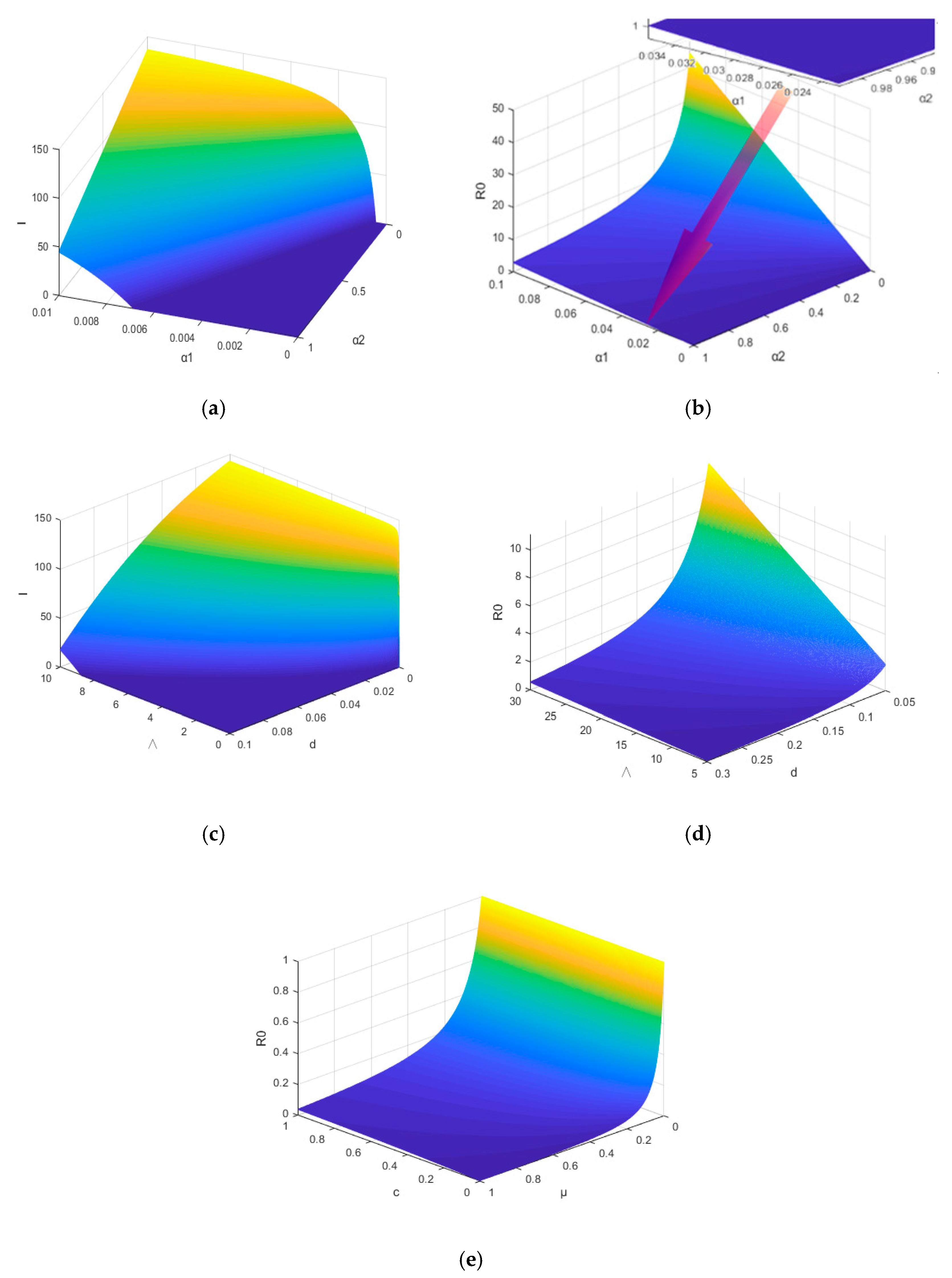
The parameter settings are given as follows in Figure 2a: $\wedge =10,d=0.05,\mu =c=0.02 and {\alpha }_1\in \left[0, 0.1\right],{\alpha }_2\in \left[0, 1\right].$ The phenomenon could be found that if the infection rate ${\alpha }_1$ is at a very low level, the spread of malware will not prevail. If ${\alpha }_2$ increases, the virus will break out. The self-recovery rate can hardly inhibit the spread of the virus if ${\alpha }_1$ is larger than 0.006.

The parameter settings are given as follows in Figure 2b: $\wedge =2,d=0.05,\mu =c=0.02 and {\alpha }_1\in \left[0, 0.1\right],{\alpha }_2\in \left[0, 1\right].$ From the enlarged picture in the upper right corner, a slight increase of ${\alpha }_1$ may lead to the prevalence of the viruses. If ${\alpha }_1\ge 0.34$, ${\alpha }_2$ can hardly adjust the spread of the viruses. Moreover, if ${\alpha }_2$ is not large enough, viruses are extremely prone to outbreak.

The parameter settings are given as follows in Figure 2c: ${\alpha }_1=0.002,{\alpha }_2=0.03,\mu =c=0.02 and \wedge \in \left[0, 10\right],d\in \left[0, 0.1\right];$ and in Figure 2d: ${\alpha }_1=0.002,{\alpha }_2=0.03, \mu =c=0.02, \wedge \in \left[5, 30\right],d\in \left[0.05, 0.3\right]$. $\wedge \mathrm{and}d$ are analyzed in Figure 2c,d to reveal the influence on the prevalence of the virus. Figure 2c shows that if d is small enough, $\wedge$ is more likely to cause a virus outbreak. As shown in Figure 2d, to keep the virus from spreading, the larger the node mortality rate d is, the wider the allowable range of injection rate $\wedge$ is.

The parameter settings are given as follows in Figure 2e: $\wedge =2, d=0.05, {\alpha }_1=0.002,{\alpha }_2=0.03, and c\in \left[0, 1\right], \mu \in \left[0, 1\right]$. The charging rate $c$ and the conversion rate of low-energy nodes $\mu$ have no decisive effect on whether the virus breaks out or not.

6.2. Stability of Equilibrium Point

The parameter settings are given as follows in Figure 3: $\wedge =10,d=0.12,{\alpha }_1=0.002,{\alpha }_2=0.03,\mu =c=0.02 and S\left(0\right)\in \left[30, 84\right],I\left(0\right)\in \left[30, 39\right],L\left(0\right)=0$. It can be found that the initial values of states will not change the convergence of the system. It is noted that S(∞), I(∞), L(∞) = 72.9167, 0, 10.4167. Even if the number of initial infected nodes is relatively large, the system virus will eventually disappear as long as $R_0\le 1$. The results shown in Figure 3 confirm Theorem 4.

The parameter settings are given as follows in Figure 4:$\wedge =10,d=0.05,{\alpha }_1=0.002,{\alpha }_2=0.03,\mu =c=0.02 and S\left(0\right)\in \left[30,93\right],I\left(0\right)\in \left[1,10\right],L\left(0\right)=0$. It can be found that the initial values of states will not change the convergence of the system. It is noted that S(∞), I(∞), L(∞)= (50.0000, 96.9388, 14.2857). This shows that if infected nodes appear in the system (1), the virus will prevail and persist if $R_0>1$. The results in Figure 4 confirm Theorem 5.

6.3. Influence of Time Delay on Malware Propagation

In this section, the influence of time delay on the convergence is discussed.

The parameter settings are given as follows in Figure 5: $\wedge =10,d=0.05, {\alpha }_1=0.002,{\alpha }_2=0.03, \mu =c=0.02$ and $S\left(0\right)\in \left[30, 84\right],I\left(0\right)\in \left[1, 10\right],L\left(0\right)=0,\tau =10$. The delay term will not affect the convergence of the system in Figure 5b. Because of the introduction of $\mathsf{\tau }$, the convergence values will have a very small wave, as shown in Figure 4a and Figure 5a. Two groups of convergence values from the system (1) and the system (26) will get closer and closer as time passes. As shown in Figure 5b, different delay values only affect the convergence speed.

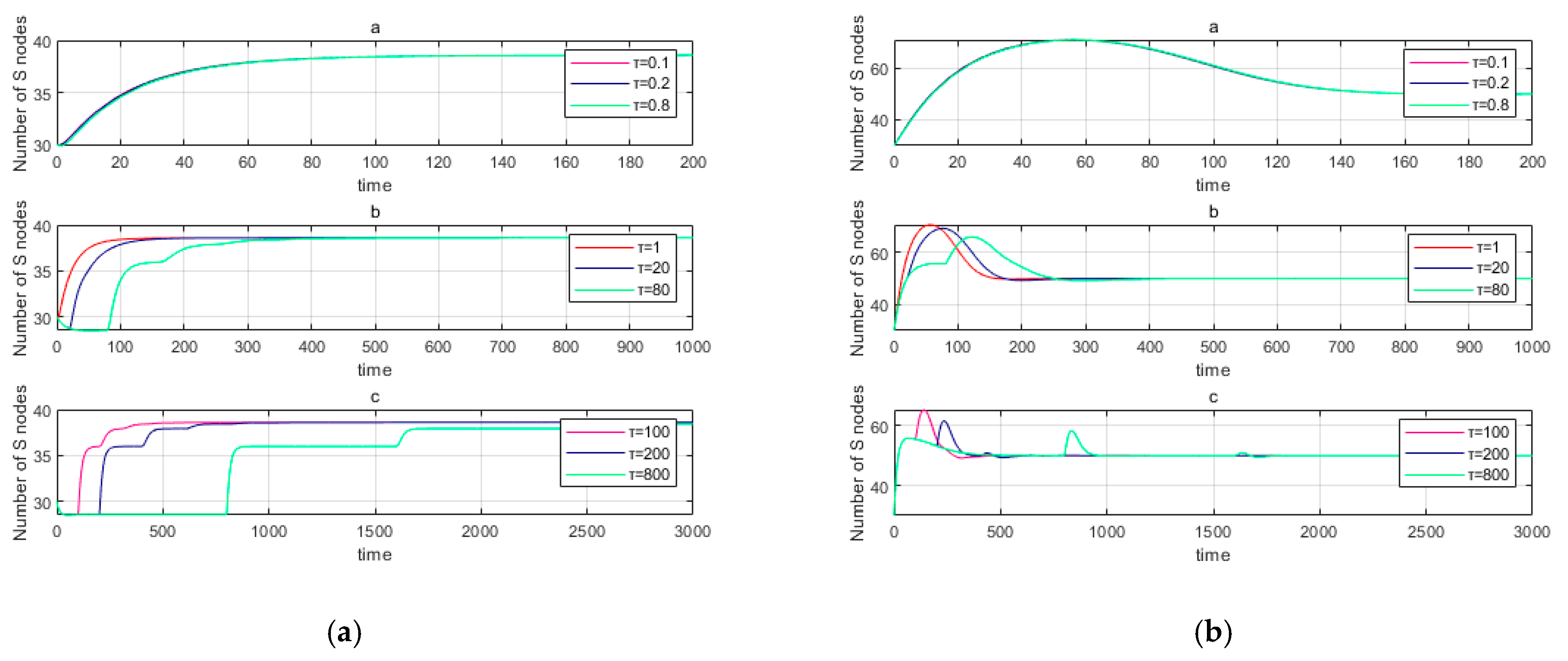
As shown in Figure 6, with the small delay item $\tau$(0.1–0.8), the delay of the S nodes’ convergence is not obvious. However, it is concerning that if $R_0< 1$ in Figure 6a, the S nodes will be in the zero-quantity state for a period under the effect of large time delay item $\tau$(100–800), which should be avoided by increasing charging power to reduce the time delay. If $R_0>1$ in Figure 6b, the delay term will only introduce the speed influence of convergence.

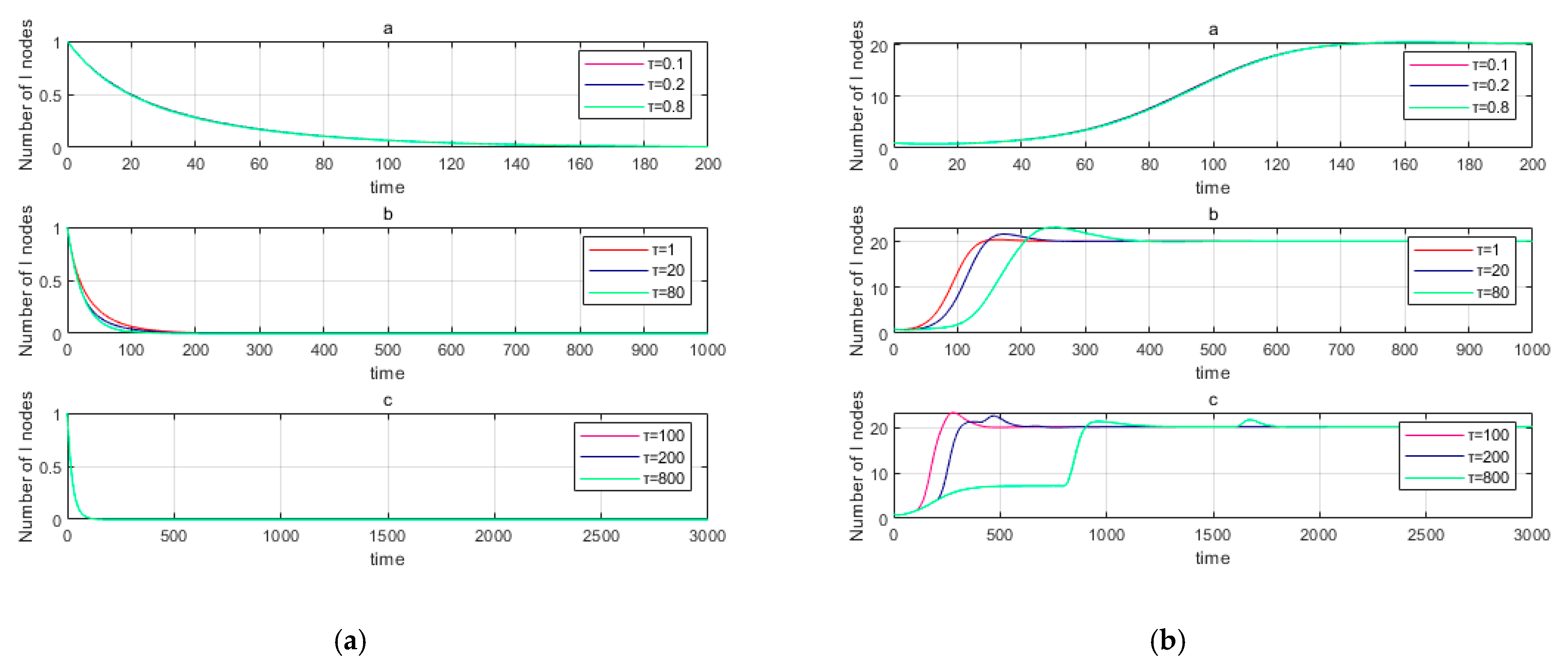
As shown in Figure 7a, the different time-delay terms have little effect on the convergence of the I node if $R_0< 1$. As shown in Figure 7b, I nodes will go through a sudden explosion period in the process of convergence under the influence of a large time delay $\tau$(200–800) if $R_0> 1$.

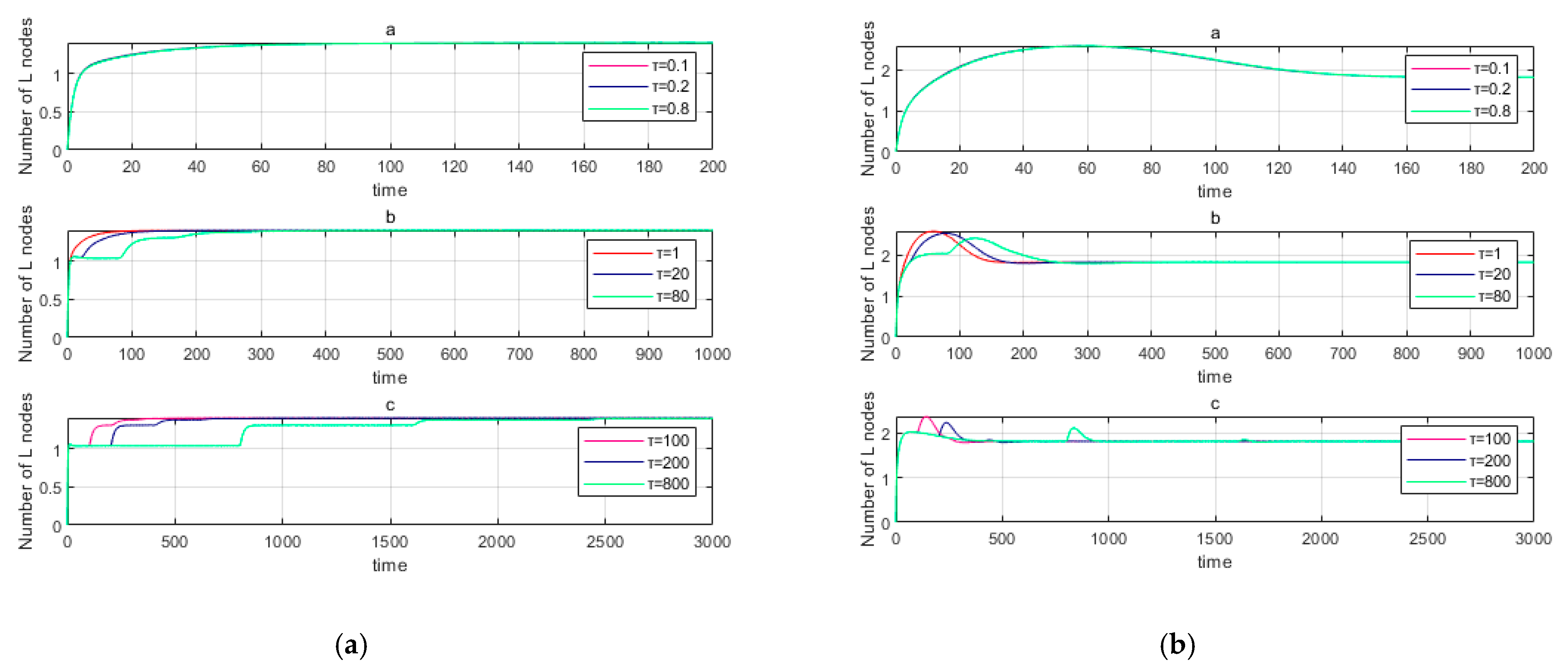
As shown in Figure 8, similarly, the delay term does not affect the convergence value but delays the convergence process obviously. It is worth noticing that the time-delay term will bring a fluctuation of the convergence process in Figure 8b if $R_0> 1$.

6.4. Realization of Optimal Control

The flowchart of simulation implementation is shown in Figure 9. It shows that the objective function converges through iterations: ($G\left(u\right)=J\left(u^k\right), \left|\frac{J\left(u^{k+1}\right)-J(u^k)}{J(u^k)}\right|<\epsilon ,\epsilon >0$). The intervention treatment ratio $u^k$ (t) is obtained.

Optimal-control simulation parameters are shown as follows: $\wedge =1,d=0.05,{\alpha }_1=0.02,{\alpha }_2=0.03,\mu =c=0.02 and S\left(0\right)=40,I\left(0\right)=20,L\left(0\right)=0$.

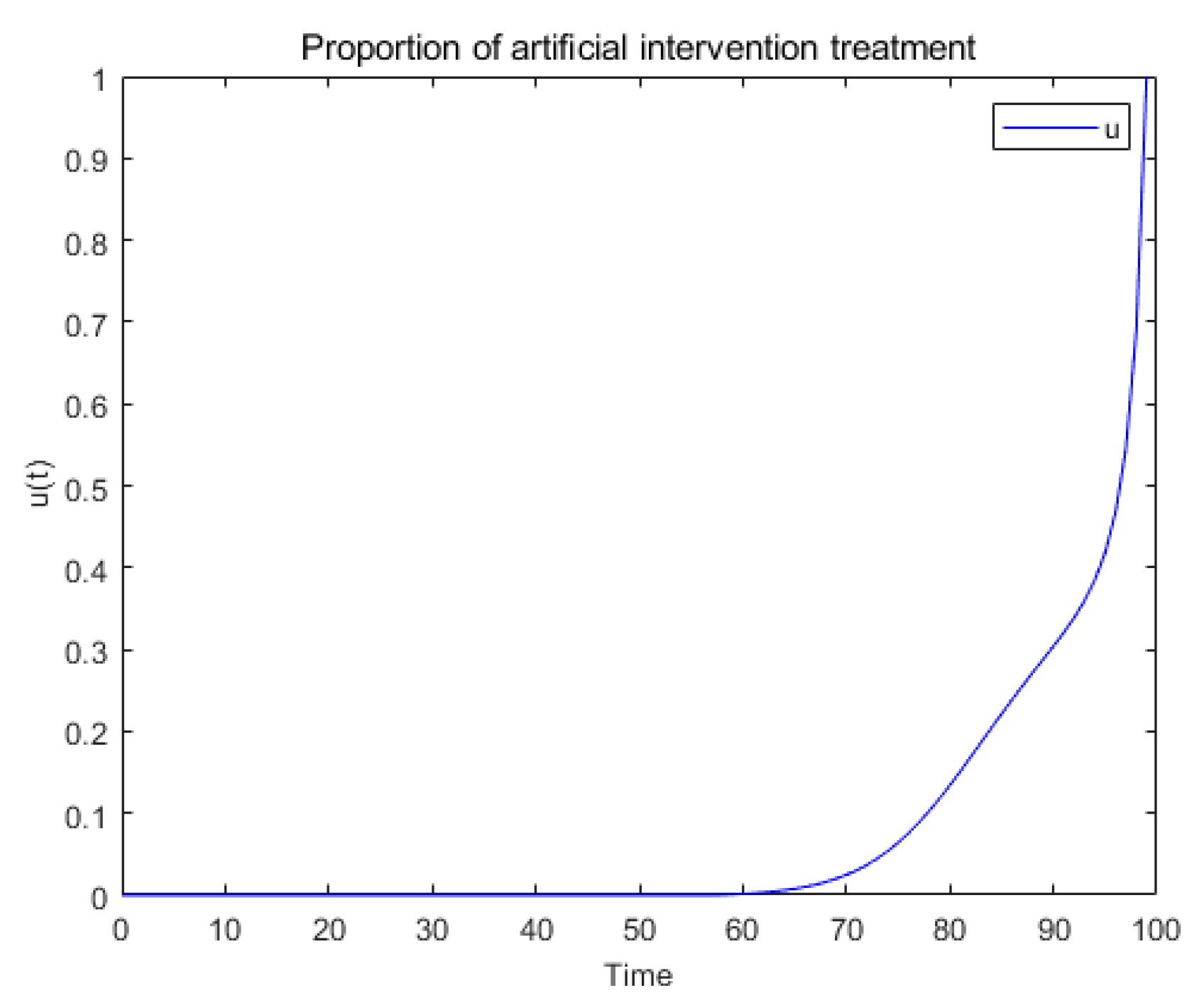
Figure 10 shows the convergence of the system without intervention treatment. It can be seen that systemic viruses are always prevalent. Figure 11 presents the optimal intervention-treatment proportion. The optimal intervention-treatment curve is zero at the beginning, and gradually increases to a value of 1.

To better compare the economic utility brought by the optimal control, state variable values at the terminal time (tf = 200) in Figure 12a are adjusted to be close to the state variable values in Figure 12b. The fixed treatment coefficient in Figure 12a is u(t) = 0.3. Comparing the size of J calculated by the objective function (20), the cost J in Figure 13b is 32.0104. However, the cost J in Figure 13a is 1901.5. Combined with the state variable values at the terminal time of Figure 12b, the strategy under optimal control not only stops the spread of the virus, but also greatly reduces the cost required by the security policy.

7. Conclusions

To better inhibit the spread of viruses, a novel epidemic model of virus spreading in WRSNs was developed after taking the time delay of the charging process into consideration. The local stability and global stability of the disease-free equilibrium point and the epidemic equilibrium point were proved by defining the basic regeneration number and the application of the Routh criterion. In addition, we concluded that the time-delay term would not change the convergence of the system, but would only affect the convergence speed. It is worth noting that Figure 6a shows that if ${\mathrm{R}}_0$ < 1, the time delays will make the S nodes zero for a while, which will greatly affect the normal operation of the network. In terms of parameter relationships, they can reflect the benefits of the modified SILS model in Figure 2e. It shows that the increase of charging power will not make the virus spread out of control, which is different from the SILS model. The asymptotic stability of the SISL model was strictly verified in simulation. At the same time, we verified the effectiveness of the proposed optimal control strategy, which not only effectively controlled the spread of the virus, but also greatly reduced the maintenance cost. The SISL model considers the influence of time delay and provides a new research perspective. We hope the results of this paper can provide some reference for related researchers.

References

1. Rawat, P.; Singh, K.D.; Chaouchi, H.; Bonnin, J.M. Wireless Sensor Networks: A Survey on Recent Developments and Potential Synergies. J. Supercomput. 2014, 68, 1–48. [Google Scholar] [CrossRef]
2. Liang, C.J.M.; Musăloiu-e, R.; Terzis, A. Typhoon: A Reliable Data Dissemination Protocol for Wireless Sensor Networks. In European Conference on Wireless Sensor Networks; Springer: Berlin/Heidelberg, Germany, 2008; pp. 268–285. [Google Scholar]
3. Rashid, B.; Rehmani, M.H. Applications of Wireless Sensor Networks for Urban Areas: A Survey. J. Netw. Comput. Appl. 2016, 60, 192–219. [Google Scholar] [CrossRef]
4. Yetgin, H.; Cheung, K.T.K.; El-Hajjar, M.; Hanzo, L.H. A Survey of Network Lifetime Maximization Techniques in Wireless Sensor Networks. IEEE Commun. Surv. Tutor. 2017, 19, 828–854. [Google Scholar] [CrossRef]
5. Rasheed, A.; Mahapatra, R.N. The Three-Tier Security Scheme in Wireless Sensor Networks with Mobile Sinks. IEEE Trans. Parallel Distrib. Syst. 2010, 23, 958–965. [Google Scholar] [CrossRef]
6. Reina, D.G.; Toral, S.L.; Johnson, P.; Barrero, F. A Survey on Probabilistic Broadcast Schemes for Wireless Ad Hoc Networks. Ad Hoc Netw. 2015, 25, 263–292. [Google Scholar] [CrossRef]
7. Batista, F.K.; Martin del Rey, A.; Queiruga-Dios, A. A New Individual-Based Model to Simulate Malware Propagation in Wireless Sensor Networks. Mathematics 2020, 8, 410. [Google Scholar] [CrossRef]
8. Lin, C.; Shang, Z.; Du, W.; Ren, J.; Wang, L.; Wu, G. CoDoC: A Novel Attack for Wireless Rechargeable Sensor Networks through Denial of Charge. In Proceedings of the IEEE INFOCOM 2019-IEEE Conference on Computer Communications, Paris, France, 29 April–2 May 2019; IEEE: New York, NY, USA, 2019; pp. 856–864. [Google Scholar]
9. Encyclopedia on Ad Hoc and Ubiquitous Computing: Theory and Design of Wireless Ad Hoc, Sensor, And Mesh Networks; Agrawal, D.P., Xie, B., Eds.; World Scientific: Singapore, 2009. [Google Scholar]
10. Song, Y.; Jiang, G.P. Model and Dynamic Behavior of Malware Propagation over Wireless Sensor Networks. In International Conference on Complex Sciences; Springer: Berlin/Heidelberg, Germany, 2009; pp. 487–502. [Google Scholar]
11. Liu, G.; Peng, B.; Zhong, X. A Novel Epidemic Model for Wireless Rechargeable Sensor Network Security. Sensors 2021, 21, 123. [Google Scholar] [CrossRef] [PubMed]
12. Zhu, L.; Guan, G. Dynamical Analysis of a Rumor Spreading Model with Self-Discrimination and Time Delay in Complex Networks. Physica A Stat. Mech. Appl. 2019, 533, 121953. [Google Scholar] [CrossRef]
13. Zhu, L.; Zhao, H. Dynamical Analysis and Optimal Control for a Malware Propagation Model in an Information Network. Neurocomputing 2015, 149, 1370–1386. [Google Scholar] [CrossRef]
14. Zhang, Z.; Si, F. Dynamics of a Delayed SEIRS-V Model on the Transmission of Worms in a Wireless Sensor Network. Adv. Differ. Equ. 2014, 2014, 1–15. [Google Scholar] [CrossRef][Green Version]
15. Liu, J.; Zhang, Z. Hopf Bifurcation of a Delayed Worm Model with Two Latent Periods. Adv. Differ. Equ. 2019, 2019, 1–27. [Google Scholar] [CrossRef]
16. Wang, C.; Chai, S. Hopf Bifurcation of an SEIRS Epidemic Model with Delays and Vertical Transmission in the Network. Adv. Differ. Equ. 2016, 2016, 1–9. [Google Scholar] [CrossRef]
17. Zhang, Z.; Wang, Y. Bifurcation Analysis for an SEIRS-V Model with Delays on the Transmission of Worms in a Wireless Sensor Network. Math. Probl. Eng. 2017, 2017, 1–15. [Google Scholar] [CrossRef]
18. Zhu, L.; Huang, X. SIS Model of Rumor Spreading in Social Network with Time Delay and Nonlinear Functions. Commun. Theor. Phys. 2019, 72, 015002. [Google Scholar] [CrossRef]
19. Zhang, Z.; Kundu, S.; Wei, R. A Delayed Epidemic Model for Propagation of Malicious Codes in Wireless Sensor Network. Mathematics 2019, 7, 396. [Google Scholar] [CrossRef]
20. Zhu, L.; Zhou, X.; Li, Y. Global Dynamics Analysis and Control of a Rumor Spreading Model in Online Social Networks. Physica A Stat. Mech. Appl. 2019, 526, 120903. [Google Scholar] [CrossRef]
21. Al-Darabsah, I. A Time-Delayed SVEIR Model for Imperfect Vaccine with a Generalized Nonmonotone Incidence and Application to Measles. Appl. Math. Model. 2020, 91, 74–92. [Google Scholar] [CrossRef]
22. Zhu, L.; Wang, X.; Zhang, H.; Shen, S.; Li, Y.; Zhou, Y. Dynamics Analysis and Optimal Control Strategy for a SIRS Epidemic Model with Two Discrete Time Delays. Phys. Scr. 2020, 95, 035213. [Google Scholar] [CrossRef]
23. Liu, G.; Peng, B.; Zhong, X.; Lan, X. Differential Games of Rechargeable Wireless Sensor Networks against Malicious Programs Based on SILRD Propagation Model. Complexity 2020, 2020, 13. [Google Scholar] [CrossRef]
24. Liu, G.; Peng, B.; Zhong, X.; Cheng, L.; Li, Z. Attack-Defense Game between Malicious Programs and Energy-Harvesting Wireless Sensor Networks Based on Epidemic Modeling. Complexity 2020, 2020, 3680518. [Google Scholar] [CrossRef]
25. Liu, G.; Peng, B.; Zhong, X. Epidemic Analysis of Wireless Rechargeable Sensor Networks Based on an Attack–Defense Game Model. Sensors 2021, 21, 594. [Google Scholar] [CrossRef] [PubMed]
26. Cooke, K.L.; van den Driessche, P. On zeroes of some transcendental equations. Funkc. Ekvacioj 1986, 29, 77–90. [Google Scholar]
Figure 1. Flow diagram of the SISL model.
Mathematics 09 00978 g001
Figure 2. The relationships of parameters. (a) The relationships among α 2 , α 1 , and I. (b) The relationships among α 2 , α 1 , and R 0 . (c) The relationships among ,   d , and I. (d) The relationships among ,   d , and R 0 . (e) The relationships among c , μ , and R 0 .
Mathematics 09 00978 g002
Figure 3. Variations of S, I, and L if R 0 = 0.8578 . (a) R 0 = 0.8578 ; two-dimensional diagram of stability. (b) R 0 = 0.8578 ; three-dimensional diagram of stability.
Mathematics 09 00978 g003
Figure 4. Variations of S, I, and L if R 0 = 3.1111 . (a) R 0 = 3.1111 ; two-dimensional diagram of stability. (b) R 0 = 3.1111 ; three-dimensional diagram of stability.
Mathematics 09 00978 g004
Figure 5. Convergences under time delay. (a) Convergence under time delay τ = 10. (b) Convergence speed under different time delays.
Mathematics 09 00978 g005
Figure 6. Convergence situations of S nodes. (a) R 0 = 0.7719 ; the convergence of S nodes under time delay. (b) R 0 = 1.5439 ; the convergence of S nodes under time delay.
Mathematics 09 00978 g006
Figure 7. Convergence situations of I nodes. (a) R 0 = 0.7719 ; the convergence of I nodes under time delay. (b) R 0 = 1.5439 ; the convergence of I nodes under time delay.
Mathematics 09 00978 g007
Figure 8. Convergence situations of L nodes. (a) R 0 = 0.7719 ; the convergence of L nodes under time delay. (b) R 0 = 1.5439 ; the convergence of L nodes under time delay.
Mathematics 09 00978 g008
Figure 9. Flowchart of optimal control.
Mathematics 09 00978 g009
Figure 10. The convergence of the system without intervention treatment.
Mathematics 09 00978 g010
Figure 11. Convergence curve of intervention treatment under the optimal control.
Mathematics 09 00978 g011
Figure 12. Comparison of economic utility between fixed intervention treatment and intervention treatment under optimal control. (a) SIL curve under the fixed proportion of intervention treatment. (b) SIL curve under the optimal control intervention treatment.
Mathematics 09 00978 g012
Figure 13. The comparison of costs. (a) The cost under the fixed treatment ratio. (b) The cost under the optimal control.
Mathematics 09 00978 g013