1. Introduction
Appell polynomials have many applications in various disciplines: probability theory [
1,
2,
3,
4,
5], number theory [
6], linear recurrence [
7], general linear interpolation [
8,
9,
10,
11,
12], operators approximation theory [
13,
14,
15,
16,
17]. In [
18], P. Appell introduced a class of polynomials by the following equivalent conditions:
is an Appell sequence (
being a polynomial of degree
n) if either
or
where
.
Subsequentely, many other equivalent characterizations have been formulated. For example, in [
19] [p. 87], there are seven equivalences.
Properties of Appell sequences are naturally handled within the framework of modern classic umbral calculus (see [
19,
20] and references therein).
Special polynomials in two variables are useful from the point of view of applications, particularly in probability [
21], in physics, expansion of functions [
22], etc. These polynomials allow the derivation of a number of useful identities in a fairly straightforward way and help in introducing new families of polynomials. For example, in [
23] the authors introduced general classes of two variables Appell polynomials by using properties of an iterated isomorphism related to the Laguerre-type exponentials. In [
24], the two-variable general polynomial (2VgP) family
has been considered, whose members are defined by the generating function
where
.
Later, the authors considered the two-variable general Appell polynomials (2VgAP) denoted by
based on the sequence
, that is
where
.
These polynomials are framed within the context of monomiality principle [
24,
25,
26,
27].
Generalizations of Appell polynomials can be also found in [
22,
28,
29,
30,
31] (see also the references therein).
In this paper, we will reconsider the 2VgAP, but with a systematic and alternative theory, that is matrix calculus-based. To the best of authors knowledge, a systematic approach to general bivariate Appell sequences does not appear in the literature. New properties are given and a general linear interpolation problem is hinted. Some applications of the previous theory are given and new families of bivariate polynomials are presented. Moreover a biorthogonal system of linear functionals and polynomials is constructed.
In particular, the paper is organized as follows: in
Section 2 we give the definition and the first characterizations of general bivariate Appell polynomial sequences; in
Section 3,
Section 4 and
Section 5 we derive, respectively, matrix form, recurrence relations and determinant forms for the elements of a general bivariate Appell polynomial sequence. These sequences satisfy some interesting differential equations (
Section 6) and properties (
Section 7). In
Section 8 we consider the relations with linear functional of linear interpolation.
Section 9 introduces new and known examples of polynomial sequences. Finally,
Section 10 contains some concluding remarks.
We point out that the first recurrence formula and the determinant forms, as well as the relationship with linear functionals and linear interpolation, to the best of authors’ knowledge, do not appear in the literature.
We will adopt the following notation for the derivatives of a polynomial
fA set of polynomials is denoted, for example, by , where the subscripts represent the (total) degree of each polynomial. Moreover, for polynomial sequences, we will use the notation for univariate sequence and in the bivariate case. Uppercase letters will be used for particular and well-known sequences.
2. Definition and First Characterizations
Let
be the power series
(usually
) and let
be the two-variable real function defined as
where
are real polynomials in the variable
y, with
.
It is known ([
19], p. 78) that the power series
generates the univariate Appell polynomial sequence
such that
Now we consider the bivariate polynomals
with real variables. We denote by
, or simply
where there is no possibility of misunderstanding, the set of bivariate polynomial sequences
such that
In the following, unless otherwise specified, the previous hypotheses and notations will always be used.
Remark 1. We observe that in [21,32] a polynomial sequence is said to satisfy the Appell condition if This sequence in [32] is used to obtain an expansion of bivariate, real functions with integral remainder (generalization of Sard formula [33]. Nothing is said about the theory of this kind of sequences. Proposition 1. A bivariate polynomial sequence is an element of if and only if Proof. If
, relations (4a) hold. Then, by induction and partial integration with respect to the variable
x ([
19] p. 93), we get relation (
5), according to (
3). Vice versa, from (
5), we easily get (4a). □
Proposition 2. A bivariate polynomial sequence is an element of if and only if Proof. If
, from Proposition 1 the identity (
5) holds. Then
From the Cauchy product of series, according to (
1) and (
2), we get (
6). Vice-versa, from (
6) we obtain (
5). Therefore relations (4a) hold. □
We call the function exponential generating function of the bivariate polynomial sequence.
Remark 2. From Propositions 1 and 2 we note explicitly that relations (4a) are equivalent to the identity (6). Example 1. Let , that is , . Then , constructed as in Proposition 1, or, equivalently, Proposition 2, is a polynomial sequence in one variable, with elements Therefore is a univariate Appell polynomial sequence [18,19]. Example 1 suggests us the following definition.
Definition 1. A bivariate polynomial sequence , that is a polynomial sequence satisfying relations (4a) or relation (6), is calledgeneral bivariate Appell polynomial sequence.
Remark 3.(Elementary general bivariate Appell polynomial sequences) Assuming , that is , , , relations (4a) become Moreover, the univariate Appell sequence is . Hence, from (5), In this case, we call the polynomial sequence elementary bivariate Appell sequence. We will denote it by , that is The set of elementary bivariate Appell sequences will be denoted by , or . Of course, . We observe that the set coincides with the set of 2VgP considered in [24]. We note that is a set of linearly independent polynomials in .
Proposition 3. Let and . Then, the following identities hold Proof. From (
9),
. Hence the result follows from (
1), (
6) and the Cauchy product of series. □
It is known that ([
19] p. 11) the power series
is invertible and it results
with
defined by
The identity (
9) (with
) yelds
with
The polynomial sequence is called conjugate bivariate Appell polynomial sequence of .
Observe that the bivariate polynomial sequence is an element of the set .
3. Matrix Form
We denote by
the infinite lower triangular matrix [
19,
34] with
and let
be the inverse matrix. It is known ([
19] p. 11) that
where
are defined as in (
12).
Observe that the matrices
A and
B can be factorized ([
19] p. 11) as
where
is a factorial diagonal matrix and
,
are lower triangualar Toeplitz matrices with entries, respectively,
and
,
.
We denote by and the principal submatrices of order n of A and B, respectively.
Let
P and
R be the infinite vectors
Moreover, for every
, let
Proposition 4. The following matrix identities hold: Proof. Identities (
15a) follow directly from (
11). The relations (
15b) follow from (
15a). □
The identities (
15a) are called
matrix forms of the bivariate general Appell sequence and we call
A the related associated matrix.
Now, we consider the vectors
By combining (
16a) and the second in (
15a) we obtain
If
and
, we get the inverse formulas
Remark 4. For the elementary Appell sequence with given in (10), we observe that the associated matrix isthat is the known Pascal matrix [12]. Hence the inverse matrix is Then we can obtain the conjugate sequence, . Therefore, from (16a) and (16b), we get If we introduce the vectorswe get the matrix identities Combining this with (15a) we get with .
Since the matrix is invertible, we get from (10) Formulas (20) and (22) are the inverse each other. In order to determine the generating function of the sequence we observe that Consequently, the generating function of isthat is is an element of . Proposition 5. For the conjugate sequence the following identity holds Proof. From (
24) and (
17a) we get
By applying the Cauchy product of series to the left-hand term in (
26), and substituting (
17a) in the right-hand term, we obtain (
25). □
4. Recurrence Relations
In [
35] has been noted that recurrence relations are a very interesting tool for the study of the polynomial sequences.
Theorem 1 (Recurrence relations)
. Under the previous hypothesis and notations for the elements of the following recurrence relations hold:with defined as in (12) and given as in (23b). Proof. The proof follows easily by identities (
15a) and (
21). □
We call relations (
28) and (
29), first and second recurrence relations, respectively.
The third recurrence relations can be obtained from the generating function.
Theorem 2 (Third recurrence relation)
. For the elements of the following identity holds: where and are such that Proof. Partial differentiation with respect to the variable
t in (
6) gives
Hence we get
and from this, relation (
30) follows. □
The same techniques used previously can be used to derive recurrence relations for the conjugate sequence. Particularly, the third recurrence relation is similar to (
30) by exchanging
with
,
, being
such that
Remark 5. Observe that if , the recurrence relation (30) becomes a three-terms relation. 5. Determinant Forms
The previous recurrence relations provide determinant forms [
36,
37], which can be useful for both numerical calculations and new combinatorial identities.
Theorem 3 (Determinant forms)
. For the elements of the following identities hold: Proof. For
relation (
28) can be regarded as an infinite lower triangular system in the unknowns
. By solving the first
equations by Cramer’s rule, after elementary determinant operations we get (
34). Relation (
35) follows from (
29) by the same technique. □
We note that the determinant forms are Hessenberg determinants. It is known ([
19] p. 28) that Gauss elimination for the calculation of an Hessenberg determinant is stable.
Theorem 4 (Third determinant form)
. For the elements of the following determinant form holds: Proof. The result follows from (
30) with the same technique used in the previous Theorem. □
We point out that the first and second recurrence relations and the determinant forms (
34)–(
36) do not appear in the literature. They will be fundamental in the relationship with linear interpolation.
Remark 6. For the elements of an expression similar to (36) is obtained by exchanging with , , being defined as in (33). Remark 7. For the elements of , from (17a), we get the recurrence relation By the same technique used in the proof of Theorem 3 we obtain the following determinant form From (30) we obtainwhere are defined as in (31). The related determinant form is 6. Differential Operators and Equations
The elements of a general bivariate Appell sequence satisfy some interesting differential equations.
Proposition 6. For the elements of the following identity holds Proof. The proof follows easily after k partial differentiation of (7b) with respect to x. □
Theorem 5 (Differential equations)
. The elements of satisfy the following differential equations Proof. The results follow by replacing relation (
39) in the first recurrence relation (
28) and in the second recurrence relation (
29), respectively. □
Theorem 6. The elements of satisfy the following differential equation Proof. The result follows by replacing relation (
39) in (
27). □
We observe that the results in Theorems 5 and 6 are new in the literature.
In order to make the paper as autonomous as possible, we remind that a polynomial sequence
is said to be quasi-monomial if two operators
and
, called multiplicative and derivative operators respectively, can be defined in such a way that
If these operators have a differential realization, some important consequences follow:
differential equation: ;
it , then , and this yields the series definition for ;
the exponential generating function of is
For the general bivariate Appell sequence we also have multiplicative and derivative operators.
Theorem 7 (Multiplicative and derivative operators [
24])
. For multiplicative and derivative operators are respectivelywhere and .Thus the set is quasi-monomial under the action of the operators and .
Proof. Relations (
41a) and (
41b) follow from (
32) and (4b), respectively [
24,
38]. □
Theorem 8 (Differential identity)
. The elements of a general bivariate Appell sequence satisfy the following differential identity Proof. From (
41a) we get the first identity. The second equality follows by (
40b), according to Theorem 7. □
Remark 8. The operators (41a) and (41b) satisfy the commutation relation [24] and this shows the structure of a Weyl group. Remark 9. From Theorem 7 and Remark 8 we get that can be interpreted as a differential equation.
7. General Properties
The general bivariate Appell polynomial sequences satisfy some properties.
Proposition 7 (Binomial identity)
. Let . The following identity holds Proof. From the generating function
Thus the result follows. □
Proof. The proof follows from Proposition 7 for and and from (4c). □
Corollary 3 (Forward difference)
. For we get Remark 10. Proposition 7 suggests us to consider general Appell polynomial sequences with three variables. In fact, setting in (42) andthe sequence can be consider a general Appell polynomial sequence in three variables. Analogously, we can consider Appell polynomial sequences in d variables with . Proposition 8 (Integration with respect to the variable
x)
. For we get Proof. Relation (
43) follows from (4b). The (
44) is obtained from (7c), (7b) and Proposition 7 for
,
. □
Proposition 9 (Partial matrix differentiation with respect to the variable
x)
. Let be the vector defined in (14). Thenwhere D is the matrix with entries Proof. The proof follows from (4b). □
In order to give an algebraic structure to the set
, we consider two elements
and
. From (
11) we get,
,
That is, with is the associated matrix to , and with is the associated matrix to .
Then we define
and we set
Proposition 10 (Umbral composition)
. The polynomial sequence , with defined as in (45), is a general bivariate Appell sequence and we call it umbral composition of and . Proof. It’s easy to verify that the matrix associated to the sequence
is
. In fact
with
.
Moreover
V is an Appell-type matrix [
19]. In fact
□
The set with the umbral composition operation is an algebraic structure .
Let be the group of infinite, lower triangular matrix with the usual product operation.
Proposition 11 (Algebraic structure). The algebraic structure is a group isomorphic to .
Proof. We have observed that is an algebraic structure. Then we have
- (i)
the elementary Appell sequence is the identity in .
- (ii)
for every the conjugate sequence is its inverse.
□
Remark 11. Given , with , if and are two elements of , the sequence is also an element of . Hence the algebraic structure is an algebra on ( or ![Mathematics 09 00964 i001]()
).
8. Relations with Linear Functional and Linear Interpolation
Let
. We consider the set of polynomials
where
,
, are defined as in (
10). Let
L be a linear functional on
. If we set
we can consider the general bivariate Appell polynomial sequence in
as in (
34) and we call it the
polynomial sequence related to the functional L. We denote it by
.
Now we define the
linear functionals
,
in
as
where in the second relation we have applied (7b).
Theorem 9. For the elements of the bivariate general Appell sequence the following identity holdswhere is the known Kronecker symbol. Proof. The proof follows from the first determinant form (Theorem 3). □
Corollary 4. The bivariate general Appell polynomial sequence is the solution of the following general linear interpolation problem on Proof. The proof follows from Theorem 9 and the known theorems on general linear interpolation problem [
39] since
,
, are linearly independent functionals. □
Theorem 10 (Representation theorem)
. For every the following relation holds Proof. The proof follows from Theorem 9 and the previous definitions. □
9. Some Bivariate Appell Sequences
In order to illustrate the previous results, we construct some two variables Appell sequences. As we have shown, to do this, for each sequence we need two power series and , where y is considered as a parameter.
Example 2.Let . There are several choices for .
- (1)
.
In this case, the elementary bivariate Appell sequence is the classical bivariate monomials. These polynomials are known in the literature also as Hermite polynomials in two variables and denoted by [40,41]: Figure 1 provides the graphs of the first four polynomials. The matrix form is obtained by using the known Pascal matrix [34]. From (25) we get the conjugate sequence hence, from (17a) and (17b), the inverse relations are Note that from (46a) and (46b) we obtain the basic relations for binomial coefficients ([42] p. 3). From (46b) we get the second recurrence relation and the related determinant form for From this we can derive many identities. For example, for , - (2)
.
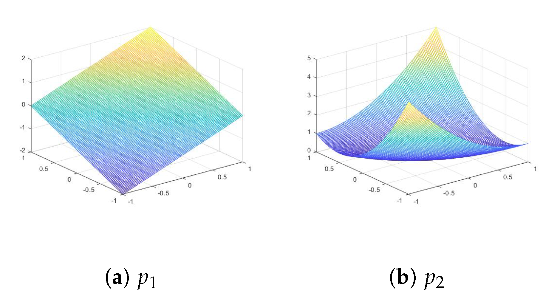
It is known ([19] p. 107) that this power series generates the univariate Bernoulli polynomials. Hence, directly from (11) we obtain a general bivariate Appell sequence which we call natural bivariate Bernoulli polynomials and denote it by , where and are, respectively, the Bernoulli polynomial of degree j and the j-th Bernoulli number ([19] p. 109). From the second equality in (47) and the known properties of Bernoulli polynomials ([19] p. 109) we have The first natural bivariate Bernoulli polynomials are Figure 2 shows the graphs of the first four polynomials , . From (11), (12) and (47) we get and Therefore the first recurrence relation is The related determinant form for is For the coefficients of we find Moreover, , , . Hence the third recurrence relation is The related determinant form for is - (3)
.
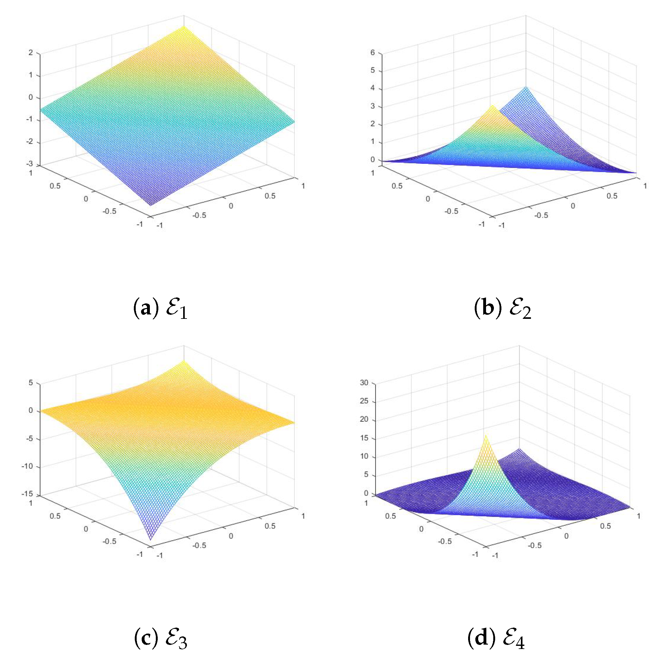
This power series generates the univariate Euler polynomials ([19] p. 123). Hence, directly from (11) we obtain a general bivariate Appell sequence which we call natural bivariate Euler polynomials and denote it by , where is the Euler polynomial of degree j ([19] p. 124). The first natural bivariate Euler polynomials are Figure 3 shows the graphs of the first four polynomials , . From (11), (12) and (49) we get , hence ([19] p. 124) and Therefore the first recurrence relation is The related determinant form for is For the coefficients of the power series we find Hence the third recurrence relation becomes The related determinant form for is
For other choices of we proceed in a similar way.
Example 3.Let . We can consider the power series as in the previous example.
- (1)
.
In this case we obtain the Hermite-Kampé de Fériet polynomials. They are denoted by , [23,28,40]. From (9) we get The first polynomials are: Particular cases are
- (a)
, known as probabilistic Hermite univariate polynomials [19] (p. 134); - (b)
, known as physicist Hermite or simply Hermite polynomials [19] (p. 134); - (c)
;
- (d)
From (13) we obtain the conjugate sequence and the second recurrence relation: The related determinant form for is From (50) for and we have Observe that . Therefore the third recurrence relation becomes The related determinant form for is To the best of authors knowledge the first recurrence relation, the first determinant form and the last determinant form are new.
For and we get the identity From the comparison with (51) the following identity is obtained: The Hermite-Kampé de Fériet polynomials satisfy the following differential equations
- 1.
;
- 2.
(heat equation);
- 3.
.
- (2)
.
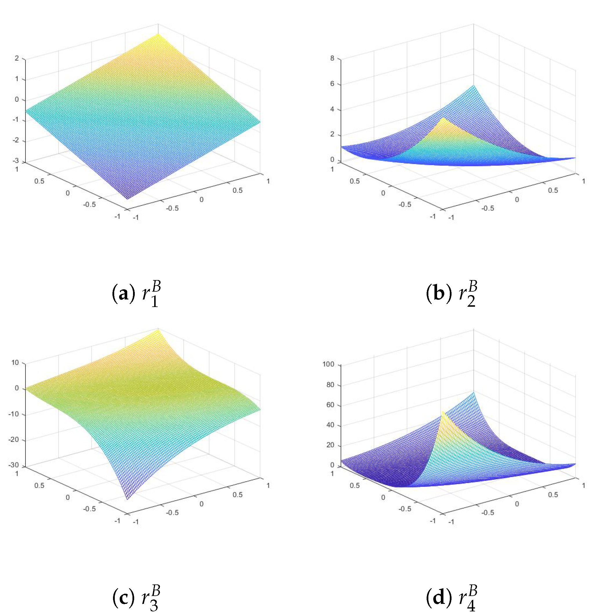
In this case we get the bivariate Appell sequence whose elements can be called Bernoulli–Hermite–Kampé de Fériet polynomials and denoted by .
From (6) and (11) we obtain The first bivariate Bernoulli–Hermite–Kampé de Fériet polynomials are In this case we observe that .
The first recurrence relation is The related determinant form is obtained from (48) by replacing by , . As we observed, for , , , , . Moreover, as in the Example 2, case 2), Hence the third recurrence relation is The related determinant form for is - (3)
.
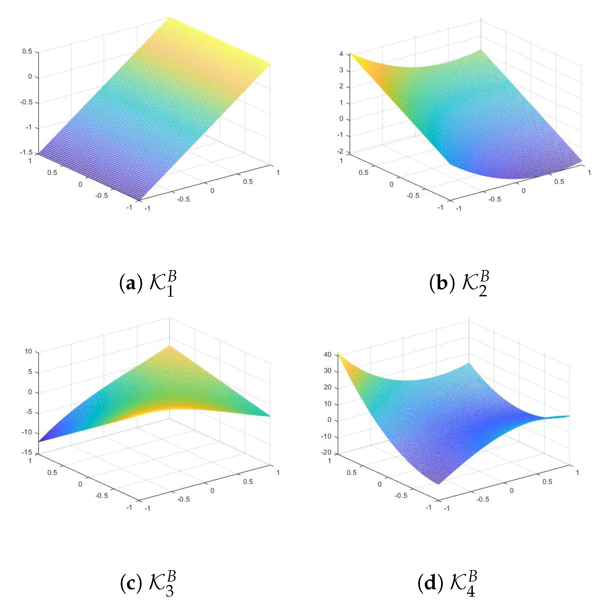
In this case we get the bivariate Appell sequence whose elements can be called Euler–Hermite–Kampé de Fériet polynomials and denoted by . with as in (52). The first polynomials of the sequence are Since , , from (12) we get , , . Therefore, the first recurrence relation is Since in this case , the third recurrence relation is The related determinant form for is
Example 4.Let .
- (1)
.
Being , from (10) we get the elementary bivariate Appell sequence and from (25) the conjugate sequence The first polynomials of the sequence are For relations (37) and (38) hold. Furthermore, since , then , . Hence, from Remark (7), for - (2)
.
Moreover, and from (12) Hence the first recurrence relation is and the conjugate sequence is The first polynomials of the sequence are As in the case (2) of the previous Examples, Hence the third recurrence relation is The related determinant form for is - (3)
. In this case we obtain The first polynomials of the sequence are Moreover, since , , , the first recurrence relation is and the conjugate sequence is As in the case (3) of the previous Examples, . Hence the third recurrence relation is The related determinant form for is
Remark 12. In [29,30] the authors introduced the functions , . They studied the related elementary sequences and respectively the Bernoulli and Genocchi sequences but matricial and determinant forms are not considered. Most of their results are a consequence of our general theory. 10. Concluding Remarks
In this work, an approach to general bivariate Appell polynomial sequences based on elementary matrix calculus has been proposed.
This approach, which is new in the literature [
3,
22,
24,
27,
28], generated a systematic, simple theory. It is in perfect analogy with the theory in the univariate case (see [
19] and the references therein). Moreover, our approach provided new results such as recurrence formulas and related differential equations and determinant forms. The latter are useful both for numerical calculations and for theoretical results, such as combinatorial identities and biorthogonal systems of linear functionals and polynomials. In particular, after some definitions, the generating function for a general bivariate Appell sequence is given. Then matricial forms are considered, based on the so called elementary bivariate Appell polynomial sequences. These forms provide three recurrence relations and the related determinant forms. Differential definitions and recurrence relations generate differential equations. For completeness of discussion the multiplicative and derivatives differential operators are hinted. A linear functional on
is considered. It generates a general bivariate Appell sequence. Hence, an interesting theorem on representation for any polynomial belonging to
is established. Finally, some examples of general bivariate Appell sequences are given.
Further developments are possible. In particular, the extension of the considered linear functional to a suitable class of bivariate real functions and the related Appell interpolant polynomial. These interpolant polynomials can be applied not only as an approximant of a function, but also to generate new cubature and summation formulas. It would also be interesting to consider the bivariate generating functions for polynomials.


 ).
).