Spatiotemporal Econometrics Models for Old Age Mortality in Europe

Abstract

In the past decade, panel data models using time-series observations of several geographical units have become popular due to the availability of software able to implement them. The aim of this study is an updated comparison of estimation techniques between the implementations of spatiotemporal panel data models across MATLAB and R softwares in order to fit real mortality data. The case study used concerns the male and female mortality of the aged population of European countries. Mortality is quantified with the Comparative Mortality Figure, which is the most suitable statistic for comparing mortality by sex over space when detailed specific mortality is available for each studied population. The spatial dependence between the 26 European countries and their neighbors during 1995–2012 was confirmed through the Global Moran Index and the spatiotemporal panel data models. For this reason, it can be said that mortality in European population aging not only depends on differences in the health systems, which are subject to national discretion but also on supra-national developments. Finally, we conclude that although both programs seem similar, there are some differences in the estimation of parameters and goodness of fit measures being more reliable MATLAB. These differences have been justified by detailing the advantages and disadvantages of using each of them.

1. Introduction

At present, spatial econometric methods are evolving very rapidly at both a theoretical and practical level. Spatial econometrics studies the spatial autocorrelation and spatial structure in regression models for cross-sectional and panel data [1]. These models have been applied in various fields such as sociology, epidemiology, geology, biology, economics, and criminology [2] but less in the field of actuarial science. Nonetheless, its importance in assessing the variation of risk in non-life insurance as a function of a geographical area has been recognized [3]. Further extensions of the spatial modeling related to frequency and severity of claims include models such as [4,5,6].

In the context of life insurance, the disaggregation of overall mortality at some levels, for example, by spatial or socio-economic factors, of mortality measures should be considered in modeling and forecasting according to [7]. In this sense, joint mortality models have been used, such as [8] and references therein.

Even though Debón et al. [9] used some spatial techniques on residuals to forecast dynamic life tables, the importance of the spatial effect has not been well recognized in modeling and forecasting dynamics of mortality. In recent years, there has been research on multi-population mortality models, for example, using a group of countries with similar social-economic status, or males and females in the same population [10]. However, these models do not measure spatial dependence and temporal and spatial effects obtained with data panel models. These methods consider panel regression models with spatially autocorrelated dependent variables and errors with fixed effects (FE) and random effects (RE) specifications.

On the other hand, Debón et al. [11] concluded that there are notable differences in mortality between the Eastern and Western of Europe, a significant disadvantage for Eastern Europe, and especially for males in Baltic countries. Therefore, it is interesting to see if we can explain these differences in mortality through a model including covariables.

For that task, there is extensive literature supporting software that estimates cross-sectional spatial models in R and MATLAB; however, few methods estimate panel data spatiotemporal models. Nevertheless, the increased availability of data, and in particular panel data, has stimulated tremendous methodological progress in studies on the specification and estimation of spatiotemporal panel data models. This interest has gone hand-in-hand with developing new packages to model spatial dependence over time in panel data such as [12,13]. At present, the splm R-package [12] is available in R and the [14] code in MATLAB. They both offer access to math functions, language, statistics, and a community of users. Therefore, a quick look at MATLAB [15] and R [16] might suggest that they are relatively similar. However, a closer look at each one’s technical capabilities and assessing other vital factors, such as documentation and quality could lead to a different conclusion.

For this reason, this study aims to provide an updated comparison of estimation techniques between the implementations of spatiotemporal panel data models across MATLAB and R software in order to fit real mortality data. The case study used concerns the male and female mortality of the aged population of European countries. Mortality is quantified with the Comparative Mortality Figure, which is the most suitable statistic for comparing mortality by sex over space when detailed specific mortality is available for each studied population [17]. In this context, the use of Generalized Linear Models (GLM) can be traced back to the early 1980s thanks to the work of [18] being suitable for the distribution of the number of deaths.

The article is structured as follows. In Section 2, we describe the data, Comparative Mortality Figure, Global Moran’s Index, and panel data models. Next, in Section 3, we present the main results, and models implemented in R and MATLAB. Section 4 provides a discussion about the most important results. Finally, in Section 5 the main conclusions of the study are drawn.

2. Materials and Methods

This section first describes the structure of the data used and how they were obtained. Secondly, it reviews the methodology employed, mainly relying on data panel models.

2.1. Data

The database used comprises deaths and populations of 26 European countries from the Human Mortality Database (HMD) [19] for the period 1995–2012, an age range of 65–110+ and male (m) and female (f) sexes. The available European countries are Austria (AT), Belgium (BE), Belarus (BY), The Czech Republic (CZ), Denmark(DK), Estonia (EE), Finland (FI), France (FR), Germany (DE), Hungary (HU), Ireland (IE), Italy (IT), Latvia (LV), Lithuania (LT), Luxembourg (LU), The Netherlands (NL), Norway (NO), Poland (PL), Portugal (PT), Slovakia (SK), Slovenia (SI), Spain (ES), Sweden (SE), Switzerland (CH), The United Kingdom (UK), and Ukraine (UA). In previous studies, Carracedo et al. [20] quantified the dynamics of mortality in Europe and detected two significant clusters for ages older than 64. In this paper, to explain the behavior of mortality as a function of socioeconomic variables, information about four variables for these 26 countries and 18 years was obtained from The World Bank Database [21]. These variables are the Gross Domestic Product (GDP), public health expenditure, CO₂ emissions, and education expenditure based on a literature review of this area [22,23,24] and data availability for European countries from [21]. In addition, there are recent studies examining the impact of CO₂ emissions, health expenditure, and education on life expectancy [24]. Furthermore, it is essential to point out that the new impacts of environmental degradation on human health affect today’s society both in terms of loss of quality of life and spending on health care. The definitions of the variables can be found below:

• Gross Domestic Product per capita (current U.S. dollars) (GDP) is an economic variable used as a measure of income. It is defined as the sum of gross value added by all resident producers in the economy plus any product taxes and minus any subsidies not included in the products’ value. GDP has traditionally been used to show the economic and social development of countries [25]. In recent years, there has been significant interest in the relationship between health, proxied by life expectancy, and income, as explained by [26], preceded by [27]. It has generally been well accepted that populations in countries with higher GDP levels have better health and longer life expectancy, as higher living standards lead to enhanced prevention and treatment of disease [27]. It should be noted that all variables are expressed in per capita values.
• Public health expenditure per capita (% of total health expenditure) (PHE) is a social variable that consists of recurrent and capital spending from government (central and local) budgets, external borrowings and grants (including donations from international agencies and nongovernmental organizations), and social (or compulsory) health insurance funds. In countries with high income per capita, the contributions to social security are essential and sustain, to a great extent, the financing of the health system. Consequently, the lower the mortality in a country, the healthier its population [28]. Several studies, such as [29,30], among others, have shown that health expenditure has a significant negative impact on mortality rate and a positive impact on life expectancy. It should be noted that the health expenditure variable is reported until 2012; for this reason, the study is limited to that year.
• CO₂ emissions per capita (metric tons) is an environmental variable that is used to indicate the effect of air pollution on mortality. Carbon dioxide emissions are those stemming from the burning of fossil fuels and the manufacture of cement. They include carbon dioxide produced during the consumption of solid, liquid, and gas fuels and gas flaring. Countries with higher carbon dioxide emissions levels are at higher risk of their citizens having health problems [24,31].
• Education Expenditure per capita (% Gross National Income) (EE) refers to the current operating expenditure on education, including wages and salaries and excluding capital investments on buildings and equipment. This variable is an essential factor that determines health as a measure of educational level. People with higher educational levels have better jobs, higher incomes, and lower-risk behavior [32].

Gavurova [33] is the closest study to our analysis, but we should highlight three distinctive features in our study. First, we use a suitable statistic to compare mortality for each country by sex, the Comparative Mortality Figure. Second, our sample is contextualized in older European people. Hence, the reliability of our results is enhanced for retired people in Europe. In addition to studying the relationship between mortality and the covariates GDP and health expenditure, we consider the impact of CO₂ emissions and education expenditure per capita over mortality. Third, we consider the neighborhood relationships between countries over time. This point is vital since studies such as Carracedo et al. [20] show that European mortality has a spatial dependence.

2.2. Comparative Mortality Figure

The Comparative Mortality Figure (CMF) was used in this study to compare the mortality experience over time by sex and country. There are two principal standardization methods—direct and indirect—which produce Comparative Mortality Figure (CMF) and Standardized Mortality Ratio (SMR), respectively. To compare the mortality experience over time by sex and country, the CMF was used in this study for two reasons. First, the same denominator applies in the calculations for each country, which permits comparison of the mortality experience by sex for different places, and second, the age-specific mortality rates are available for each country [17] required in the expression of CMF but not in the expression of SMR.

The CMF allows for the direct standardization method of mortality rates across age groups to permit comparison of the free effects of differences in the size of subgroups of the populations [17]. In this study, we used males (m) in the set of European countries in the year 2012 as the standard population. Therefore, the CMF is defined as follows,

$$CM{F}_{i,t,s}=\frac{E_{i,t,s}}{O_{2012,m}}i\in \{1,\dots ,26\}, t\in \{1995,\dots ,2012\},s\in \{m,f\},$$

(1)

where $E_{i,t,s}$ represents the expected deaths in country i, in year t, and sex s and $O_{2012,m}$ is the number of observed deaths in the set of European countries in year 2012 for males. As we have $d_{x,i,2012,m}$ the number of observed deaths for the age x,

$$O_{2012,m}=\sum _{i=1}^{26}\sum _{x=65}^{110+}{d}_{x,i,2012,m}x\in \{65,\dots ,110+\}.$$

Then $E_{i,t,s}$ are obtained by using the age-specific death rate of each country i for the age x, year t, and sex s, $m_{x,i,t,s}$,

$$E_{i,t,s}=\sum _{x=65}^{110+}{P}_{x,2012,m}{m}_{x,i,t,s},$$

(2)

where $P_{x,2012,m}$ is the population in the set of European countries at age x in year 2012 for $male$ sex, which can be obtained by adding all $p_{x,i,t,s}$ the population of each country i with the following expression

$$P_{x,2012,m}=\sum _{i=1}^{26}{p}_{x,i,2012,m}.$$

The death rate of the study population ($m_{x,i,t,s}$) are obtained as

$$m_{x,i,t,s}=\frac{d_{x,i,t,s}}{p_{x,i,t,s}},$$

(3)

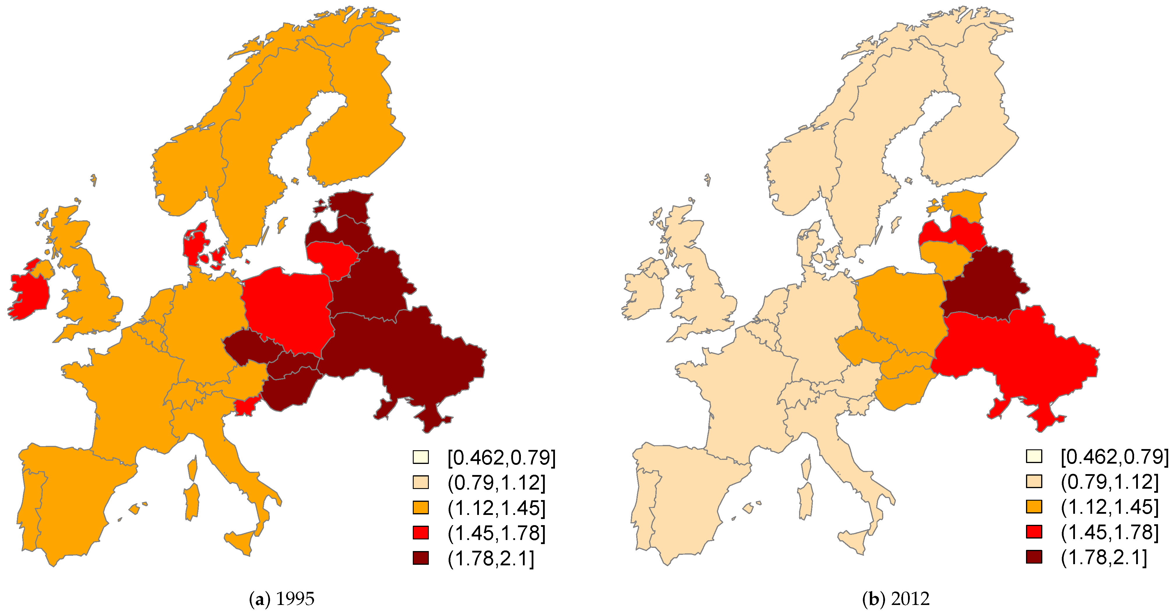
where $d_{x,i,t,s}$ and $p_{x,i,t,s}$ are the number of deaths and the study population, respectively. If the CMF is greater than 1, there is a higher expected number of deaths than observed; in this case, there are “excess deaths” in the studied countries. On the contrary, a CMF value below 1 indicates a lower expected number of deaths than observed relative to the standard population. According to [17,34], the numbers of observed deaths in the countries is a random variable that follows a Poisson distribution; in the case of CMF that distribution can be used for modelization.

2.3. Spatial Dependence of CMF

Global Moran’s Index (GM) is widely used to test for the presence of spatial dependence between adjacent locations [35,36]. In this study, it is a summary measure that shows the intensity of spatial dependence of all countries’ CMF considered.

$$G{M}_{t,s}=\frac{N}{{\displaystyle \sum _i^{}}{\displaystyle \sum _j^{}}\omega ij}\frac{{\displaystyle \sum _i^{}}{\displaystyle \sum _j^{}}\omega ij(CM{F}_{i,t,s}-{\overline{CMF}}_{g,t,s})(CM{F}_{j,t,s}-{\overline{CMF}}_{t,s})}{{\displaystyle \sum _i^{}}{(CM{F}_{i,t,s}-{\overline{CMF}}_{t,s})}^2}$$

where ${\overline{CMF}}_{t,s}$ is the mean of the CMF of all countries for each year t and sex s and $W_N$ is the neighborhood or spatial weights matrix. The definition of proximity is given by $W_N$, which is an $N\times N$ ($26\times 26$) positive matrix that provides a weight ${\omega }_{i,j}$ to each pair of spatial units $(i,j)$ [37]. In this study, the weights matrix is used in row standardized form. In addition, two countries are considered neighbors when they have a common border (first order of neighborhood [38]), and therefore, if a country is not a neighbor of itself, it takes the following values,

$$\begin{array}{ccc}\hfill {\omega }_{i,j}=0,& & \mathrm{if}j\notin V\left(i\right);\hfill \\ \hfill {\omega }_{i,j}=\frac{1}{n_i},& & \mathrm{if}j\in V\left(i\right),\mathrm{with}{n}_i=\#V\left(i\right);\hfill \\ \hfill {\omega }_{i,i}=0,& & i=1\dots 26.\hfill \end{array}$$

where $n_i$ is the number of neighbors of country i and $V\left(i\right)$ the set of neighbors of the country i. The interpretation for $G{M}_{t,s}$ is the following:

• $G{M}_{t,s}>0$—Positive spatial autocorrelation between countries. The CMF of countries and their neighbors goes in the same direction.
• $G{M}_{t,s}>0$—Negative spatial autocorrelation between countries. The CMF of countries and their neighbors varies in a different direction.
• $G{M}_{t,s}=0$—Absence of spatial autocorrelation between the 26 European countries, meaning a random spatial pattern.

Moran’s test for spatial autocorrelation was calculated to test the significance of the GM index. The null hypothesis establishes that the $CM{F}_{i,t,s}$ is randomly distributed among the spatial units of the study area $(H_0:G{M}_{t,s}=0)$ [39].

2.4. Spatiotemporal Panel Data Models

The analysis of data from the spatiotemporal panel is currently a field of econometrics undergoing significant methodological advances [12]. Panel data consist of a cross-section of observations (individuals, countries, regions) followed through time. Specifically, the data from this study are panel data that combine a spatial dimension N (26 countries) and temporal dimension T (18 years). In a spatiotemporal panel, there may be dependency or correlation between the close observations (spatial units) over time (temporal units).

Econometrics panel data models offer advantages over cross-section regression or time series as they control for unobserved heterogeneity produced by both spatial and temporal units. As a result, these models reduce the issues related to multicollinearity problems between the variables by building more efficient estimates in the parameters of the panel data models [40]. Panel data usually contain more degrees of freedom and more sample variability, combining both cross-sectional and time-series data, hence, improving the efficiency of econometric estimates [41]. The spatiotemporal panel data models are used as the regression models that employ the panel structure’s temporal and spatial heterogeneity to estimate parameters of interest [42].

Due to the nature of our variables, we propose a log–log spatiotemporal panel data model that assumes the log transformation of the CMF and the explanatory variables to achieve approximate normality and symmetry about the distribution of CMF and provide straightforward interpretability of the results [43]. In this model, the explanatory variables’ coefficients represent the elasticity of CMF for the explanatory variables [44].

The spatial lag term considers that the value of the CMF in a country depends on the value of the CMF in its vicinity. This fact will be confirmed in Section 3.2. In addition, the fixed effects model is generally more appropriate than the random effects model when the sample used is fixed, i.e., the countries have not been drawn randomly from a very large population [37]. In our case, we would like to model the space-time data of adjacent spatial units (countries) or “located in an unbroken study area” [45]. For these reasons, we fitted spatial lag models with fixed effects. This model fits the behavior of CMF by country and time as a function of explanatory variables assuming that the differences between spatial units, time units, or both are constant [46]. For this reason, spatial and temporal dummy variables were created to account for the unobserved characteristics of cross-sectional units (not changing with time but affecting the dependent variable) and the unobserved characteristics of temporal units (not changing with countries but affecting the dependent variable). These models use the notation that has become usual in this context and adapted to explain the log transformation of CMF, namely,

• Spatial Lag Model (SLM):

  $$log\left(CM{F}_{it}\right)=\alpha +\lambda (I_T\otimes W_N)log\left(CM{F}_{it}\right)+log\left(X_{it}\right)\beta +{ϵ}_{it}$$
• Spatial Lag Model with spatial fixed effects (SLMSFE);

  $$log\left(CM{F}_{it}\right)=\alpha +\lambda (I_T\otimes W_N)log\left(CM{F}_{it}\right)+log\left(X_{it}\right)\beta +{\mu }_i+{ϵ}_{it}$$

  (4)
• Spatial Lag Model with time fixed effects (SLMTFE);

  $$log\left(CM{F}_{it}\right)=\alpha +\lambda (I_T\otimes W_N)log\left(CM{F}_{it}\right)+log\left(X_{it}\right)\beta +{\nu }_t+{ϵ}_{it}$$
• Spatial Lag Model with spatial and time fixed effects (SLMSTFE);

  $$log\left(CM{F}_{it}\right)=\alpha +\lambda (I_T\otimes W_N)log\left(CM{F}_{it}\right)+log\left(X_{it}\right)\beta +{\mu }_i+{\nu }_t+{ϵ}_{it}$$

where $log\left(CM{F}_{it}\right)$ represents an ordered vector of dimension $\left(26\right)\left(18\right)\times 1$ corresponding to observations of the dependent variable for each country i and year t, $\alpha$ is the intercept, $\lambda$ is the spatial parameter associated with the dependent variable, $log\left(X_{it}\right)$ represents a matrix of dimension $\left(26\right)\left(18\right)\times 4$, the log transformation of the explanatory variables ordered by spatial units first and then by time period, which are related to the parameters $\beta$ of dimension $4\times 1$. The fixed effects considered in the model are as follows:

• ${\mu }_i$ is the spatial fixed effect (not spatially autocorrelated), which captures the unobservable characteristics that change across countries but remain constant over time.
• ${\nu }_t$ is the temporal fixed effect (not temporally autocorrelated), which captures the unobservable characteristics that change over time but remain constant across countries.

$\lambda$ denotes the spatial autoregressive parameter on the spatially lagged dependent variable to follow the econometrics literature [47,48]. SLMSTFE has the conditions that the sum of the spatial and temporal effects are zero [49]. These conditions are achieved using 26 spatial dummies and 18 time dummies because 26 and 18 are the total number of countries and years considered in this study. Thus, the spatial effect represents the deviation of the spatial unit i from the mean $\alpha$, and the time effect represents the deviation of the time unit t from the mean $\alpha$.

On the other hand, GLMs are an extension of linear models for response variables with non-normal distributions and nonlinear transformations [18]. GLM provides a method for estimating a function of the dependent variable’s mean, also called link function, as a linear combination of a set of explanatory variables. Poisson regression is a GLM model where the dependent variable is a count that follows a Poisson distribution. The canonical link results in a log-linear relationship between mean and linear predictor. The Poisson model variance is identical to the mean; thus, in the case the variance is larger than the mean, the data are over-dispersed.

A way of modeling over-dispersed count data is to use the quasi-Poisson model, which produces the same coefficient estimates as the standard Poisson model, but the inference is adjusted over-dispersion. Consequently, the quasi-Poisson family does not correspond to a model with fully specified likelihood, and therefore, statistical tests and goodness-of-fit measures such as AIC, BIC, likelihood-ratio are unavailable in the output of model [16]. In R, the quasi-Poisson model with estimated dispersion parameter can also be fitted with the glm function and setting family = quasipoisson.

We suggest adapting log–log SLMSTFE to GLM, the model proposed for $log\left(CMF\right)$ is,

$$log\left(\frac{E_{i,t,s}}{O_{2012,m}}\right)=\alpha +\lambda (I_T\otimes W_N)log\left(CM{F}_{it}\right)+log{X}_{it}\beta +{\mu }_i+{\nu }_t+{ϵ}_{it}.$$

(5)

In the next section, these models are estimated by maximum likelihood with splm and glm functions in R software and the sar_panel_FE function in MATLAB. In this way, the glm function takes into account the value of the quasiPoisson-likelihood and not the log-likelihood value.

3. Results

3.1. Exploratory Analysis of the CMF

A preliminary study of the temporal evolution of the CMF of European countries for males and females is discussed in this section. Firstly, the CMF of men and women in Europe from 1995 and 2012 was represented on the maps. These maps are all comparable to each other as the color scale is the same for all these figures using the corresponding common quartiles of all years and both sexes.

Figure 1 shows the CMF in Europe for the years 1995 and 2012 for males. It should be noted that the CMF of men for the year 1995 in Europe has a value higher than 1.12, which is exceptionally high for the eastern countries, followed by Ireland, Denmark and, finally, the rest of the western ones. Its evolution for 2012 shows lower values than in 1995, with a minimum of 0.462 reached in the western countries, followed by some eastern countries and incredibly high for Belarus.

The same analysis for females is shown in Figure 2. The value of CMF for 1995 in Europe ranges between 0.462 and 1.45, lower than in males. In 2012, the female CMF decreased so that it reached at most 1.12 for the second quintile of the scale in eastern countries.

Secondly, CMF variability was explored for both sexes versus the countries and the years. Figure 3 shows the comparison of the CMF range for males and females in all countries. The countries were ordered alphabetically, and a higher average value and variability were confirmed for men, especially in the eastern countries. Figure 4 shows the comparison of the CMF range for males and females in all years. Again, higher variability in men than in women was detected, while a decreasing trend was observed in both sexes.

After the exploratory analysis of the CMF, the next step was to test the significance of mortality dependence on space where the null hypothesis is no spatial correlation.

3.2. Spatial Dependence of CMF

The Moran tests for each year are shown in

Table 1. Values of the Global Moran’s I and p-values by sex.

Year	${\mathit{GM}}_{\mathit{t},\mathit{s}}$		p-Value
	Male	Female	Male	Female
1995	0.7181	0.7114	2.7969 $\times {10}^{-6}$	3.4530 $\times {10}^{-6}$
1996	0.7237	0.7093	2.3057 $\times {10}^{-6}$	3.4908 $\times {10}^{-6}$
1997	0.7278	0.7131	1.9082 $\times {10}^{-6}$	3.0991 $\times {10}^{-6}$
1998	0.7215	0.7397	2.4848 $\times {10}^{-6}$	1.5671 $\times {10}^{-6}$
1999	0.7034	0.7050	3.6203 $\times {10}^{-6}$	3.6449 $\times {10}^{-6}$
2000	0.6961	0.6962	4.1529 $\times {10}^{-6}$	4.2046 $\times {10}^{-6}$
2001	0.7346	0.7007	1.3305 $\times {10}^{-6}$	3.6365 $\times {10}^{-6}$
2002	0.7266	0.6920	1.4161 $\times {10}^{-6}$	4.1134 $\times {10}^{-6}$
2003	0.7305	0.6816	1.4139 $\times {10}^{-6}$	5.1248 $\times {10}^{-6}$
2004	0.7556	0.7090	6.5537 $\times {10}^{-7}$	2.6387 $\times {10}^{-6}$
2005	0.7681	0.7134	4.4887 $\times {10}^{-7}$	2.1915 $\times {10}^{-6}$
2006	0.7747	0.7210	3.7009 $\times {10}^{-7}$	1.6916 $\times {10}^{-6}$
2007	0.7883	0.7186	2.6180 $\times {10}^{-7}$	1.8677 $\times {10}^{-6}$
2008	0.7856	0.7169	2.5542 $\times {10}^{-7}$	1.6588 $\times {10}^{-6}$
2009	0.7829	0.7150	2.7193 $\times {10}^{-7}$	1.8195 $\times {10}^{-6}$
2010	0.7617	0.7017	4.7935 $\times {10}^{-7}$	2.4996 $\times {10}^{-6}$
2011	0.7728	0.6951	3.3224 $\times {10}^{-7}$	3.0838 $\times {10}^{-6}$
2012	0.7764	0.6995	3.1847 $\times {10}^{-7}$	2.7272 $\times {10}^{-6}$

for males and females. The p-values obtained for all years are significant (p-values < 0.05), indicating a spatial dependence between the mortality of the 26 countries in the period 1995–2012 in both sexes.

3.3. Spatiotemporal Panel Data Models

After testing the significance of mortality dependence, the next step was fitting spatiotemporal panel data models.

3.3.1. Fitting Spatiotemporal Panel Data Models

Parameter estimation for the spatiotemporal panel data models described in Section 2.4 were performed using the splm and glm functions of splm and stats R-packages, respectively. It is important to note that the version of the splm R-package used was 1.5–2, which produces the same parameter estimates as version 1.3–7. At present, versions other than the two mentioned are not correct because model fitting does not work well. Regarding MATLAB software, the sar_panel_FE function of demopanelscompare file was used.

It is essential to mention that the dataset’s structure for fitting the spatiotemporal panel data models is different depending on the software used. In R, both the dependent and the independent variables are ordered by spatial units first and then by time. On the other hand, in MATLAB, all variables are ordered by time first, then by spatial units.

A summary of the results of the spatiotemporal panel data models together with the corresponding goodness-of-fit measures by sex are shown in

Table 2. Model fittings using the splm function in R by sex.

Sex	Model	$\mathit{\alpha }$	$\mathit{\lambda }$	log(GDP)	log(CO2)	log(EE)	log(PHE)	logLik
Male	SLM
	SLMSFE	1.436 *	0.814 *	−0.038 *	0.054 *	0.050 *	0.034 *	145.081
	SLMTFE	1.677 *	0.420 *	−0.136 *	0.086 *	0.017 *	0.010 *	−213.404
	SLMSTFE	0.361 *	0.430 *	0.076 *	−0.024 *	0.038 *	0.031 *	249.972
Female	SLM
	SLMSFE	2.826 *	0.544 *	−0.100 *	0.118 *	0.061 *	0.110 *	−32.906
	SLMTFE	1.486 *	0.374 *	−0.148 *	0.100 *	0.011 *	0.018 *	−343.423
	SLMSTFE	1.135 *	0.063 *	0.009 *	−0.001 *	0.040 *	0.071 *	49.788

* p-values < 0.05; Items in bold are showing the differences in the sign of the parameter estimation respect to Table 4.

for splm function in R,

Table 3. Model fittings using the sar_panel_FE function in MATLAB by sex.

Sex	Model	$\mathit{\alpha }$	$\mathit{\lambda }$	log(GDP)	log(CO2)	log(EE)	log(PHE)	${\mathit{R}}^2$	log-Likelihood	${\mathit{\sigma }}^2$
Male	SLM	1.592 *	0.460 *	−0.131 *	0.089 *	0.014 *	0.012 *	0.906	550.241	0.0051
	SLMSFE	1.479 *	0.806 *	−0.040 *	0.057 *	0.051 *	0.036 *	0.986	904.110	0.0008
	SLMTFE	1.680 *	0.419 *	−0.136 *	0.086 *	0.017 *	0.010 *	0.909	561.217	0.0051
	SLMSTFE	0.370 *	0.468 *	0.072 *	−0.023 *	0.038 *	0.030 *	0.988	1024.73	0.0007
Female	SLM	1.433 *	0.406 *	−0.144 *	0.102 *	0.008 *	0.020 *	0.851	424.616	0.0089
	SLMSFE	2.901 *	0.524 *	−0.103 *	0.123 *	0.062 *	0.114 *	0.964	735.632	0.0023
	SLMTFE	1.478 *	0.379 *	−0.147 *	0.100 *	0.011 *	0.018 *	0.855	431.176	0.0091
	SLMSTFE	1.148 *	0.108 *	0.007 *	−0.001 *	0.040 *	0.008 *	0.971	824.475	0.0019

* p-values < 0.05; Items in bold are showing the differences in the sign of the parameter estimation respect to Table 4.

for sar_panel_FE function in MATLAB and

Table 4. Model fittings using the glm function in R by sex.

Sex	Model	$\mathit{\alpha }$	$\mathit{\lambda }$	log(GDP)	log(CO2)	log(EE)	log(PHE)	Residual Deviance
Male	SLM	1.346 *	0.540 *	−0.112 *	0.070*	0.004 *	0.017 *	3.371
	SLMSFE	0.490 *	0.982 *	−0.004 *	−7.081$\times {\mathbf{10}}^{-\mathbf{5}}$	0.042 *	−7.453$\times {\mathbf{10}}^{-\mathbf{5}}$	0.453
	SLMTFE	1.422 *	0.517 *	−0.117 *	0.070 *	−0.002 *	0.020 *	3.258
	SLMSTFE	0.356 *	0.760 *	0.037 *	−0.020 *	0.041 *	0.013 *	0.430
Female	SLM	1.157 *	0.505 *	−0.122 *	0.084 *	−0.008 *	0.029 *	3.494
	SLMSFE	1.932 *	0.760 *	−0.052 *	0.054 *	0.053 *	0.078 *	0.814
	SLMTFE	1.227 *	0.480 *	−0.128 *	0.083 *	−0.009 *	0.031 *	3.419
	SLMSTFE	1.161 *	0.122 *	0.012 *	−0.010 *	0.042 *	0.070 *	0.692

* p-values < 0.05; Items in bold are showing the differences in the sign of the parameter estimation respect to Table 2 and Table 3.

using the glm function in R. Parameter estimations with p-values less than $5\%$ were considered significant.

The SLMSTFE is the one with the highest $R^2$ and likelihood values and lowest value of ${\sigma }^2$ in R and MATLAB. However, the spatial effect in the model has more weight than the temporal, and the inclusion of the time effect increases both goodness-of-fit measures, but not significantly. For this reason, and following the principle of parsimony, SLMSFE is the best model for both sexes.

The SLMSTFE has the lowest residual deviance value, but, as before, the SLMSFE is the best model for both sexes. In this case, only the education expenditure variable is significant for SLMSFE in males with the glm function, which simplifies the model.

Next, the results of the estimation of the spatial fixed effects of SLMSFE with MATLAB are shown in

Table 5. Estimation of spatial effects of SLMSFE model with MATLAB.

Country	Estimate ${\mathit{\mu }}_{\mathit{i}}$		t-Value		p-Value
	Male	Female	Male	Female	Male	Female
Austria	−0.151	−0.081	−0.541	−0.176	0.588	0.861
Belgium	0.013	−0.014	0.045	−0.030	0.964	0.976
Belarus	0.134	0.078	0.476	0.166	0.634	0.868
Switzerland	−0.093	−0.052	−0.332	−0.112	0.740	0.911
Czech Republic	0.082	0.126	0.289	0.267	0.772	0.789
Germany	0.164	0.352	0.495	0.639	0.621	0.523
Denmark	−0.042	−0.019	−0.156	−0.042	0.876	0.966
Estonia	−0.254	−0.488	−1.056	−1.226	0.291	0.220
Spain	0.056	0.134	0.177	0.256	0.860	0.798
Finland	−0.005	−0.146	−0.017	−0.325	0.987	0.745
France	0.065	0.132	0.200	0.246	0.841	0.806
Hungary	0.113	0.131	0.400	0.279	0.689	0.780
Ireland	0.004	−0.083	0.016	−0.190	0.987	0.850
Italy	0.088	0.213	0.272	0.396	0.786	0.692
Lithuania	−0.192	−0.250	−0.752	−0.591	0.452	0.554
Luxembourg	−0.232	−0.518	−1.061	−1.427	0.289	0.154
Latvia	−0.038	−0.094	−0.150	−0.226	0.881	0.821
Netherland	0.042	0.077	0.143	0.157	0.887	0.875
Norway	−0.090	−0.147	−0.341	−0.335	0.733	0.738
Poland	0.039	0.144	0.124	0.276	0.901	0.783
Portugal	0.118	0.124	0.414	0.262	0.679	0.794
Sweden	−0.102	−0.042	−0.368	−0.090	0.713	0.928
Slovenia	−0.079	−0.279	−0.320	−0.679	0.749	0.497
Slovakia	0.039	0.018	0.144	0.040	0.886	0.968
Ukraine	0.259	0.389	0.799	0.726	0.424	0.468
Uk	0.061	0.297	0.189	0.553	0.850	0.580

. This summary includes the model’s fixed spatial parameters, ${\mu }_i$, the t-value of these parameters, and the corresponding p-values. All spatial effects ${\mu }_i$ are not significant, but the global spatial effect is significant according with Table 3 where the inclusion of ${\mu }_i$ in SLM model increases the explanatory power of the model.

3.3.2. Validation Spatial Lag Model with Spatial Fixed Effects

The SLMSFE model was assessed using the $R^2$, the value of the log-likelihood, and ${\sigma }^2$ in MATLAB. The $R^2$ for males and females are 98.60% and 96.40%, respectively. The values of the likelihood for males and females are 904.11 and 735.63, respectively. Considering ${\sigma }^2$, its value for males is 0.0008 and females 0.0023. Since most of the variability in these models is explained, we conclude that these two models fit well. It is important to note that the corresponding $R^2$ for the ordinary least squares models by sex is 84.02% for males and 79.46% for females. These results indicate the importance of modeling the spatial correlation since the inclusion of the model’s spatial effect improves its fit by approximately 15% and 17% in males and females.

Next, residuals were analyzed to check if the SLMSFE model explains the whole spatial dependence of the 26 European countries detected by the Global Moran Index (see Section 2.3).

Table 6. Values of the Global Moran’s I and p-values by sex.

Year	${\mathit{GM}}_{\mathit{t},\mathit{s}}$		p-Value
	Male	Female	Male	Female
1995	0.031	0.082	0.334	0.232
1996	0.120	−0.069	0.166	0.568
1997	0.173	−0.033	0.797	0.473
1998	0.018	−0.114	0.448	0.730
1999	0.117	−0.037	0.680	0.493
2000	0.001	−0.001	0.403	0.407
2001	0.151	0.096	0.750	0.193
2002	0.415	0.064	0.991	0.264
2003	0.201	0.243	0.064	0.042
2004	0.363	−0.228	0.977	0.876
2005	0.167	−0.042	0.090	0.505
2006	0.201	0.014	0.071	0.371
2007	0.072	−0.185	0.577	0.813
2008	0.056	0.086	0.282	0.223
2009	0.439	−0.174	0.993	0.795
2010	0.005	−0.213	0.391	0.853
2011	0.143	−0.008	0.735	0.423
2012	0.030	−0.015	0.476	0.439

shows the result of applying the Global Moran test to the SLMSFE model residuals in 1995–2012 by sex. The p-values obtained for all years and both sexes are not significant (p-values > 0.05), indicating that non-spatial dependence remains in the residuals.

Then, in order to check that the residuals were homoscedastic in the SLMSFE model, the Breush Pagan test [50] was applied using the function bptest of lmtest package [51].

Table 7. Values of the Breusch-Pagan statistic and p-values by sex.

Model	Breusch-Pagan Test		p-Value
	Male	Female	Male	Female
SLMSFE	42.407	34.300	0.103	0.358

shows the output of Breusch-Pagan statistics and the corresponding p-values by sex. It can be observed that the p-values in the residuals of the SLMSFE model are greater than the 5% significance level for both sexes. Therefore, there was no evidence to conclude that the SLMSFE model residuals are not homoscedastic.

On the other hand, the SLMSFE model residuals have an average around zero; specifically, for males and females they are $1.232\times {10}^{-17}$ and $-4.285\times {10}^{-17}$, respectively.

Next, the normality of the SLMSFE model residuals by sex was analyzed with the function qqPlot of car R-package. Figure 5 represents the quantile–quantile (Q–Q) plot of the SLMSFE model residuals, which suggests that the error terms are normally distributed for both sexes. It should be noted that, for females, two high leverage observations were detected: observation 417, which corresponds to Slovakia in the year 1997, and observation 454, which corresponds to the UK in the year 1998.

4. Discussion

4.1. Spatiotemporal Panel Data Models

4.1.1. Comparison of Spatiotemporal Panel Data Models

Table 2 and Table 3 show very similar parameter estimations: only the second or third decimal is different between coefficients. Nevertheless, different goodness-of-fit measures were obtained in the output of the models. While the splm function comprises only the value of log-likelihood (logLik) setting quiet = FALSE, the sar_panel_FE function contains three measures by default: the value of the coefficient of determination ($R^2$), the value of the log-likelihood (log-likelihood) and the residual variance (${\sigma }^2$). The log-likelihood obtained within MATLAB versus R is more reliable as some values are negative for the latter one. It is noteworthy that the SLM model is not obtained in Table 2 because the non-fixed effect option is not possible in the argument effect of the splm function.

Table 4 shows that the values of the parameter estimation are different from those in Table 2 and Table 3. The differences in sign are marked in bold, which correspond to the variables $log\left(C{O}_2\right)$, $log\left(EE\right)$, and $log\left(PHE\right)$, which are almost always not significant. The signs of the spatial parameter and $log\left(GDP\right)$ variable remain constant using the three functions. This is due to the fact that glm assumes Poisson distribution, while the splm and sar_panel_FE assumes Normal distribution in the maximum likelihood estimation. It should be noted that there is only one measure of goodness-of-fit in the output glm, which is the residual deviation.

To incorporate the fixed effects in the function glm a reference level is set; by default, it is the first value in alphabetical order. Therefore, $\alpha$ represents the fixed effect of that country for the first year. Moreover, this reference can be changed thanks to the function contr.treatment. On the contrary, the functions splm and sar_panel_FE consider $\alpha$ as the mean because they have the conditions that the sum of the spatial and the sum of the temporal effects are zero [49]. Thus, the spatial effect represents the deviation of the spatial unit i from the mean $\alpha$, and the temporal effect represents the deviation of the temporal unit t from the mean $\alpha$.

Despite there being differences in parameter estimation and goodness-of-fit measurements using functions splm, sar_panel_FE, and glm, SLMSFE is the best for all of them. The results suggest that with sufficient social and economic variables for each country and considering the neighborhood structure, we can adequately explain any geographical structures in European mortality of old age.

4.1.2. Interpretation Spatial Lag Model with Spatial Fixed Effects

In this subsection, the SLMSFE is interpreted as being the best model using both pieces of software and the three functions. The Elhorst program code [14] in MATLAB was selected as it is considered a pioneer in including spatial dependence in panel data, and millions of engineers and scientists have tested its algorithms [52].

In the SLMSFE, all the independent variables are significant for females, with p-values less than 0.05 indicating that they all contribute significant information in explaining $log\left(CMF\right)$; in the case of males, $log\left(PHE\right)$ is not significant. Moreover, coefficients represent the percentage change in Y when the percent change in X is 1% as Equation (4) is a log–log model.

The estimate for $\alpha$ represents the average value of $log\left(CMF\right)$ when the fixed effects and explanatory variables take values equal to 0. This value is positive for males (1.479) and females (2.901). The spatial lag estimations ($\lambda$) are highly significant in both models, supporting the conjecture that the value of $log\left(CMF\right)$ in one country is influenced by the values of the $log\left(CMF\right)$ in the neighboring countries. For males, the positive values of $\lambda$ indicate that the CMF in one country would be 0.806% higher if its neighbors had a CMF average increase of 1%. In females, the $\lambda$ positive value is lower than in males; the CMF in one country would be increased by 0.524% if its neighbors had a CMF average increase of 1%. These results indicate a greater spatial dependence on male than female mortality for the aging population. Therefore, mortality in European population aging depends not only on differences on the health systems but also on supra-national developments [20].

The $log\left(GDP\right)$ coefficient indicates that with a 1% increase in GDP, the elasticity of CMF is −0.040% for males and −0.103% for females, on average. This relationship is confirmed in several studies such as the recent study by Gavurova et al. [33], among others. These authors studied the influence of socioeconomic determinants on mortality by sex in the European Union (EU) using panel data models. They confirm that GDP per capita, representing countries’ economic growth, decreases mortality in EU countries for both sexes.

With respect to $log\left(C{O}_2\right)$ emissions, the coefficient indicates that, with a 1% increase in CO₂, the elasticity of CMF is 0.057% for males and 0.123% females, on average. This result is consistent with Balan [24] among others, who studies whether there is a causal relationship between environment and health, measured by life expectancy, for EU countries. The author considers CO₂ emissions as the logical consequence of polluting industrial activities, which implies strong economic growth. The authors of [24] confirms that CO₂ emissions decrease life expectancy, thereby increasing mortality.

Finally, concerning the coefficients of two social variables $log\left(EE\right)$ and $log\left(PHE\right)$ following the literature such as [24,33], a negative relationship would be expected between overall mortality and both variables. In our study, these coefficients are positive, and in the case of $log\left(PHE\right)$ for males are not significant. There is controversy about the positive sign of both variables, which would require further investigation. However, we think that this occurs as we are studying old-age mortality.

With respect to spatial fixed effects in Table 5, it is worth mentioning that although the countries do not differ from the average $\alpha$ at least, the extremes differ between them. For both sexes, estimates with a negative sign indicate countries with lower $log\left(CMF\right)$ than the mean $\alpha$; on the contrary, the estimations of spatial effects with a positive sign belong to countries with higher $log\left(CMF\right)$. This sign means that these countries’ unobserved characteristics decrease or increase mortality compared to the all countries’ average.

4.2. Limitations

In this subsection, it is worth mentioning two critical limitations of this study. The first is the database used, which could be expanded with other socio-economics, demographic, environmental, and health variables from The World Bank Database [21]. These variables should be related to mortality and are perfectly justified with previous studies. This justification is fundamental to avoid irrelevant variables and simplify interpretability in the independent variables. On the other hand, the choice of the World Bank Database is crucial in this spatial study because it allows us to have more information on neighboring spatial units for a longer time horizon than other databases such as Eurostat.

The second limitation is that our objective is specific to mortality data. We fit spatiotemporal panel data models to real mortality data. It is not general, fitting to any data. Studying mortality has always been of interest in the actuarial and epidemiological context. However, the coronavirus disease 2019 (COVID-19) has produced unknown effects on the overall population mortality [53]. Therefore, now more than ever, mortality is attracting considerable research attention, even more so in advanced ages.

5. Conclusions

This study reproduces the sar_panel_FE function written by Elhorst [14] in MATLAB and in free software R using the splm and glm functions. R software is free and accessible to everyone, while MATLAB is commercial software with a very high price. Nevertheless, millions of engineers and scientists have tested the spatial-temporal algorithms of MATLAB; on the contrary, some functions such as splm in the splm R-package are more recent.

Therefore, this study compares MATLAB and R implementations of spatiotemporal econometrics panel data models:

• The main difference lies in the second or third decimal of estimated parameters.
• Signs and values estimated parameters differ when using the glm function in R. This is because the glm function assumes Poisson distribution, while the splm and sar_panel_FE take on Normal distribution in the maximum likelihood estimation.
• Concerning the splm function, at the present time, we have found that versions other than 1.3-7 and 1.5-2 do not correctly estimate the model parameters.
• The goodness-of-fit measures in the output are different depending on the function used. The splm function only gives the value of the log-likelihood, the sar_panel_FE function offers the values of coefficient of determination, log-likelihood, and residual variance, and the glm function the value of residual deviance.
• The log-likelihood values obtained in MATLAB are more reliable than in R because negative values appear in the latter. The tree function showed that the SLMSFE is the model that best fits the European old-age mortality data where the spatial effect is essential and the temporal one does not appear.
• An important advantage of the glm function compared to the rest is that the reference level for fixed effects can be changed. On the contrary, the splm and sar_panel_FE functions consider the reference level for fixed effects as the mean of fixed effects.

Considering other authors’ works, we should highlight the methodology’s distinctive features presented here. As far as we know, the spatiotemporal panel data models implemented by the splm R-package [12] and MATLAB [14] have not been used to study the CMF of European countries. The spatiotemporal panel data models used by [54] model mortality quantified by the Standardized Mortality Ratio (SMR) in the United States. We must point out that the CMF reflects better than the SMR the changing situation of mortality in the countries as its expression requires the age-specific mortality rates for each country. Our work could be complementary to [55], since we show the advantages and disadvantages of each function used in R and MATLAB software. Bivand and Piras [55] constitutes an exciting comparison of a generalized method of moments and maximum likelihood implementations for spatial econometrics models using MATLAB, Stata, Python, and R.

This article shows that mortality modeling should take into account both the socioeconomic characteristics underlying the modeling process and the neighborhood relationships of geographic locations. Therefore, having good, quality, socioeconomic data and correctly setting the neighborhood criterion data panel models can quantify the vast majority of the variation in European old-age mortality by country. In the changing environment in which we live, it is necessary for the authorities responsible for population planning to quantify those changes that transcend the borders of any one spatial unit. Therefore, it is of vital importance to study the mortality in Europe, especially in advanced ages. Such understanding aims to ensure the correct formulation and implementation of policies for sustainable development in Europe. In this sense, we would like to point out that although this study only applies to mortality for European countries, this methodology can be extended to the comparison of mortality of subpopulations in any geographic area when age-specific mortality rates are available for each spatial unit and a panel of covariates with the same spatial and temporal dimension as mortality.

References

1. Anselin, L. Chapter A companion to theoretical econometrics. In Spatial Econometrics; Malden, M.A., Ed.; Blackwell Publishing: Hoboken, NJ, USA, 2001; pp. 310–330. [Google Scholar]
2. Gersmehl, P. Teaching Geography, 3rd ed.; Guilford Publications: New York, NY, USA, 2014. [Google Scholar]
3. Boskov, M.; Verrall, R. Premium rating by geographic area using spatial models. Insur. Math. Econ. 1995, 3, 274. [Google Scholar] [CrossRef] [Green Version]
4. Dimakos, X.; Di Rattalma, A. Bayesian premium rating with latent structure. Scand. Actuar. J. 2002, 3, 162–184. [Google Scholar] [CrossRef]
5. Denuit, M.; Lang, S. Non-life rate-making with Bayesian GAMs. Insur. Math. Econ. 2004, 35, 627–647. [Google Scholar] [CrossRef]
6. Gschlößl, S.; Czado, C. Spatial modelling of claim frequency and claim size in non-life insurance. Scand. Actuar. J. 2007, 3, 202–225. [Google Scholar] [CrossRef] [Green Version]
7. Booth, H.; Tickle, L. Mortality modelling and forecasting: A review of methods. Ann. Actuar. Sci. 2008, 3, 3–43. [Google Scholar] [CrossRef]
8. Debón, A.; Montes, F.; Martínez-Ruiz, F. Statistical methods to compare mortality for a group with non-divergent populations: An application to Spanish regions. Eur. Actuar. J. 2011, 1, 291–308. [Google Scholar] [CrossRef] [Green Version]
9. Debón, A.; Martínez-Ruiz, F.; Montes, F. A geostatistical approach for dynamic life tables: The effect of mortality on remaining lifetime and annuities. Insur. Math. Econ. 2010, 47, 327–336. [Google Scholar] [CrossRef] [Green Version]
10. Dong, Y.; Huang, F.; Yu, H.; Haberman, S. Multi-population mortality forecasting using tensor decomposition. Scand. Actuar. J. 2020, 2020, 754–775. [Google Scholar] [CrossRef]
11. Debón, A.; Chaves, L.; Haberman, S.; Villa, F. Characterization of between-group inequality of longevity in European Union countries. Insur. Math. Econ. 2017, 75, 151–165. [Google Scholar] [CrossRef] [Green Version]
12. Millo, G.; Piras, G. splm: Spatial Panel Data Models in R. J. Stat. Softw. 2012, 47, 1–38, Version 1.5-2. Available online: http://www.jstatsoft.org/v47/i01/ (accessed on 9 February 2021). [CrossRef] [Green Version]
13. Elhorst, J.P. Chapter Spatial Panel Data Analysis. In Encyclopedia of GIS; Springer International Publishing: Cham, Switzerland, 2017; pp. 2050–2058. [Google Scholar]
14. Elhorst, J.P. Matlab Software to Estimate Spatial Panels, 2011. Version 2011-04-11. Available online: https://spatial-panels.com/software/ (accessed on 9 February 2021).
15. The MathWorks Inc. MATLAB—The Language of Technical Computing, Version 8.5.0.197613; The MathWorks Inc.: Natick, MA, USA, 2015; Available online: http://www.mathworks.com/products/matlab/ (accessed on 9 February 2021).
16. R Core Team. R: A Language and Environment for Statistical Computing; R Foundation for Statistical Computing: Vienna, Austria, 2021. [Google Scholar]
17. Julious, S.; Nicholl, J.; George, S. Why do we continue to use standardized mortality ratios for small area comparisons? J. Public Health 2001, 23, 40–46. [Google Scholar] [CrossRef] [Green Version]
18. McCullagh, P.; Nelder, J. Generalized Linear Models, 2nd ed.; Chapman and Hall: London, UK, 1989. [Google Scholar]
19. Human Mortality Database. University of California, Berkeley (USA), and Max Planck Institute for Demographic Research (Germany). Available online: www.mortality.org or www.humanmortality.de (accessed on 12 July 2016).
20. Carracedo, P.; Debón, A.; Iftimi, A.; Montes, F. Detecting spatio-temporal mortality clusters of European countries by sex and age. Int. J. Equity Health 2018, 17, 38. [Google Scholar] [CrossRef] [PubMed] [Green Version]
21. The World Bank Database. World Development Indicators; The World Bank Database: Washington, DC, USA, 2018; Data Download on 6 March 2018; Available online: https://data.worldbank.org/indicator (accessed on 9 February 2021).
22. Cutler, D.; Deaton, A.; Lleras-Muney, A. The determinants of mortality. J. Econ. Perspect. 2006, 20, 97–120. [Google Scholar] [CrossRef] [Green Version]
23. O’Hare, C.; Li, Y. Is mortality spatial or social? Econ. Model. 2014, 42, 198–207. [Google Scholar] [CrossRef] [Green Version]
24. Balan, F. Environmental quality and its human health effects: A causal analysis for the EU-25. Int. J. Appl. Econ. 2016, 13, 57–71. [Google Scholar]
25. Eurostat. Quality of Life Indicators; Eurostat: Luxemburg, 2013; Available online: http://ec.europa.eu/eurostat/statistics-explained/index.php/Quality_of_life_indicators_-_health (accessed on 9 February 2021).
26. Neofytidou, A.; Fountas, S. The impact of health on GDP: A panel data investigation. J. Econ. Asymmetr. 2020, 21, e00139. [Google Scholar] [CrossRef]
27. Swift, R. The relationship between health and GDP in OECD countries in the very long run. Health Econ. 2011, 20, 306–322. [Google Scholar] [CrossRef] [Green Version]
28. Jaba, E.; Balan, C.B.; Robu, I.B. The relationship between life expectancy at birth and health expenditures estimated by a cross-country and time-series analysis. Procedia Econ. Financ. 2014, 15, 108–114. [Google Scholar] [CrossRef] [Green Version]
29. Hitiris, T.; Posnett, J. The determinants and effects of health expenditure in developed countries. J. Health Econ. 1992, 11, 173–181. [Google Scholar] [CrossRef]
30. Shaw, J.W.; Horrace, W.C.; Vogel, R.J. The determinants of life expectancy: An analysis of the OECD health data. South. Econ. J. 2005, 71, 768–783. [Google Scholar] [CrossRef] [Green Version]
31. World Health Organization. Air Quality Guidelines: Global Update 2005: Particulate Matter, Ozone, Nitrogen Dioxide, and Sulfur Dioxide; World Health Organization: Geneva, Switzerland, 2006. [Google Scholar]
32. Mărginean, I. Public expenditure with education and healthcare in EU countries. Procedia Econ. Financ. 2014, 8, 429–435. [Google Scholar] [CrossRef] [Green Version]
33. Gavurova, B.; Khouri, S.; Kovac, V.; Ferkova, M. Exploration of influence of socioeconomic determinants on mortality in the European Union. Int. J. Environ. Res. Public Health 2020, 17, 4699. [Google Scholar] [CrossRef] [PubMed]
34. Inskip, H. Standardization methods. Encycl. Biostat. 1998, 4237–4250. [Google Scholar] [CrossRef]
35. Moran, P.A.P. Notes on continuous stochastic phenomena. Biometrika 1950, 37, 17–23. [Google Scholar] [CrossRef]
36. Moran, P.A.P. A Test for the serial independence of residuals. Biometrika 1950, 37, 178–181. [Google Scholar] [CrossRef]
37. Croissant, Y.; Millo, G. Panel Data Econometrics with R; Wiley: Hoboken, NJ, USA, 2019. [Google Scholar]
38. Anselin, L. Local Indicators of Spatial Association–LISA. Geogr. Anal. 1995, 27, 93–115. [Google Scholar] [CrossRef]
39. Cliff, A.; Ord, J. Spatial Autocorrelation; Pion: London, UK, 1973. [Google Scholar]
40. Kennedy, P. A Guide to Econometrics; MIT Press: Cambridge, MA, USA, 2003. [Google Scholar]
41. Hsiao, C.; Pesaran, M.H.; Tahmiscioglu, A.K. Maximum likelihood estimation of fixed effects dynamic panel data models covering short time periods. J. Econom. 2002, 109, 107–150. [Google Scholar] [CrossRef]
42. Elhorst, J.P. Spatial panel models. In Handbook of Regional Science; Springer: Berlin/Heidelberg, Germany, 2014; pp. 1637–1652. [Google Scholar]
43. Mendenhall, W.; Sincich, T.; Boudreau, N.S. A Second Course in Statistics: Regression Analysis; Prentice Hall: Upper Saddle River, NJ, USA, 1996; Volume 5. [Google Scholar]
44. Pindyck, R.; Rubinfeld, D. Econometric Models. Economic Forecasts., 4th ed.; McGraw-Hill: New York, NY, USA, 1991. [Google Scholar]
45. Elhorst, J.P. Spatial Econometrics: From Cross-Sectional Data to Spatial Panels; Springer: Berlin/Heidelberg, Germany, 2014. [Google Scholar]
46. Asteriou, D.; Hall, S. Applied Econometrics, 3rd ed.; Palgrave Macmillan: New York, NY, USA, 2015. [Google Scholar]
47. Kelejian, H.H.; Prucha, I.R. A generalized spatial two-stage least squares procedure for estimating a spatial autoregressive model with autoregressive disturbances. J. Real Estate Financ. Econ. 1998, 17, 99–121. [Google Scholar] [CrossRef]
48. Kelejian, H.H.; Prucha, I.R. A generalized moments estimator for the autoregressive parameter in a spatial model. Int. Econ. Rev. 1999, 40, 509–533. [Google Scholar] [CrossRef] [Green Version]
49. Hsiao, C. Analysis of Panel Data, 3rd ed.; Cambridge University Press: Cambridge, UK, 2014; p. 38. [Google Scholar]
50. Breusch, T.S.; Pagan, A.R. A simple test for heteroscedasticity and random coefficient variation. Econometrica 1979, 47, 1287–1294. [Google Scholar] [CrossRef]
51. Zeileis, A.; Hothorn, T. Diagnostic Checking in Regression Relationships. R News 2002, 2, 7–10. [Google Scholar]
52. Elhorst, J.P. Specification and estimation of spatial panel data models. Int. Reg. Sci. Rev. 2003, 26, 244–268. [Google Scholar] [CrossRef]
53. Banerjee, A.; Pasea, L.; Harris, S.; Gonzalez-Izquierdo, A.; Torralbo, A.; Shallcross, L.; Noursadeghi, M.; Pillay, D.; Sebire, N.; Holmes, C.; et al. Estimating excess 1-year mortality associated with the COVID-19 pandemic according to underlying conditions and age: A population-based cohort study. Lancet 2020, 395, 1715–1725. [Google Scholar] [CrossRef]
54. Yang, T.C.; Matthews, S.A.; Park, K. Looking through a different lens: Examining the inequality-mortality association in US counties using spatial panel models. Appl. Geogr. 2017, 86, 139–151. [Google Scholar] [CrossRef] [PubMed]
55. Bivand, R.; Piras, G. Comparing Implementations of Estimation Methods for Spatial Econometrics; American Statistical Association: Boston, MA, USA, 2015. [Google Scholar]
Figure 1. CMF in Europe for 1995 and 2012 for males.
Mathematics 09 01061 g001
Figure 2. CMF in Europe for 1995 and 2012 for females.
Mathematics 09 01061 g002
Figure 3. CMF variability in Europe for males and females.
Mathematics 09 01061 g003
Figure 4. CMF’s variability in Europe for each country for males and females.
Mathematics 09 01061 g004
Figure 5. Normality of the SLMSFE model residuals for males and females.
Mathematics 09 01061 g005