Optimal Design of High-Voltage Disconnecting Switch Drive System Based on ADAMS and Particle Swarm Optimization Algorithm

Abstract

This paper focuses on the analysis of the stability of the GW17 high-voltage disconnecting switch drive system. Firstly, the optimization model of the disconnector is established, and the simulation analysis is carried out by ADAMS (Automatic Dynamic Analysis of Mechanical Systems) and the simulation results are verified by experiments. Afterwards, ADAMS optimization design and particle swarm optimization algorithm (PSO) are used to optimize the drive system of the disconnector, and the results are verified on the experimental platform. After optimization, the space rod is reduced by 15 mm, the minimum corner angle of the lower conductive rod is reduced by 71.0%, the minimum folding arm angle is reduced by 88.7% and the maximum force of the ball pair is reduced by 35.7%, which realizes the lightweight of the rod, reduces the wear of the ball pair, and improves the stability of the equipment operation.

1. Introduction

High-voltage disconnecting switch is the most commonly used substation equipment in the power system, and plays a role of isolating voltage during power maintenance and inspection [1]. Due to long-term outdoor operation, the probability of mechanical failure is greatly increased. Common fault types in the operation of high-voltage disconnecting switch include jamming of the mechanism, heating and burning of the contact fingers, inadequate opening and closing, and breakage of the transmission connecting rod [2]. According to statistics, the mechanical defects cause more than 70% of the total faults, which seriously affect the normal operation of the power system.

At present, most scholars are focusing on remote monitoring [3], seismic resistance [4], and electrical performance [5] of high-voltage disconnecting switch. Gong et al. [6] simulated the electric field distribution in the high-voltage disconnecting switch, and optimized the design of the disconnector by response surface method. Xie et al. [7] analyzed and summarized the response law of displacement, strain and acceleration of porcelain bottle on the dynamic and static side of the disconnector under earthquake action. Through a series of laboratory tests, Y. Chai et al. [8,9,10] studied the current breaking characteristics of the disconnector, and enhanced the current breaking ability of the high-voltage disconnecting switch.

In terms of mechanical structure, Shen [11], Jiang et al. [12], etc., have done a more in-depth analysis of the transmission and extension mechanism of the high-voltage disconnector, obtained the formula and curve of folding characteristics and motion trajectory, and optimized the design of the conductive rod motion mechanism of the disconnector. In the real world, in order to solve complex optimization problems, different meta-heuristic optimization methods such as genetic algorithms, particle swarm optimization (PSO) and differential evolution algorithms have been developed and applied to many engineering optimization problems [13]. For example, truss topology optimization design [14], airfoil shape aerodynamic optimization [15], vehicle streamline optimization [16], complex system reliability optimization [17]. As the main movement and stability mechanism of the disconnector, the drive system is always difficult to achieve the ideal state in the process of engineering installation and debugging due to its multiple adjustable parameters. Therefore, it has important practical engineering significance to optimize its design, provide theoretical reference and improve equipment reliability.

Starting from the stability and safety of the opening and closing state of the disconnector, this paper establishes the mathematical model and physical model of the disconnector. Through the kinematic analysis [18,19,20], the parametric design [21,22] and optimization analysis of the drive system are carried out by using ADAMS (Automatic Dynamic Analysis of Mechanical Systems). At the same time, the PSO algorithm which is often used to solve optimization problems is selected to verify the reliability of the optimization results [23]. Then an experimental platform is built to verify the effectiveness of the optimization results.

2. Composition of Disconnector Mechanism

GW17 type disconnector is composed of switch power assembly, base assembly, insulator assembly, general switch assembly and other structures, as shown in Figure 1. The main knife switch assembly consists of a drive system and a folding arm system. The drive system is composed of a spatial four-bar linkage mechanism, and the folding arm system is composed of upper and lower conducting poles, gear rack and other mechanisms. This paper mainly studies the main switch of GW17 high-voltage disconnecting switch [17].

The working principle of the disconnector: after the motor starts to run, the output driving torque drives the rotary porcelain bottle to start to rotate. The rotating arm in the spatial four-bar linkage of the transmission base is connected with the rotating porcelain bottle, which drives the rotating arm to rotate and drives the lower conducting rod to move under the action of the spatial pull rod.The upper end of the inner tie rod is fixedly connected with the rack, which makes relative movement with the lower conducting rod, and then drives the gear rack movement, so that the upper conducting rod makes extension and folding movement with the gear relative to the lower conducting rod, and completes the opening and closing movement process.

According to the movement process of opening and closing, the main switch knife mechanism of disconnector is simplified, and the movement diagram shown in Figure 2 can be obtained: AB is the rotating arm, BC is the space rod, CDH is the fixed connection structure between the frame and the lower conducting pole, EF is the tie rod, FG is the inner tie rod, GH is the rack and pinion, and HI is the upper conducting pole. The motion diagram consists of six components and eight motion pairs (including one ball pair, one ball pin pair, five rotation pairs and one gear plane high pair). It can be seen from Equation (1) that the overall degree of freedom of the simplified mechanism diagram is one, which is consistent with the number of original moving parts, so its motion condition is uniquely determined.

$$F=6n-{\displaystyle \sum }_{i=1}^m{p}_i-{\displaystyle \sum }_{j=1}^X{q}_j-\sum R_K$$

(1)

where F is the number of degrees of freedom, n is the total number of movable components, m is the total number of motion pairs, X is the total number of prime movers, $p_i$is the number of constraint conditions of the i-th motion pair, $q_j$is the number of driving constraints of the j-th prime mover, $R_K$ is the number of other constraints.

3. Motion Model Analysis

3.1. Motion Analysis of Drive System

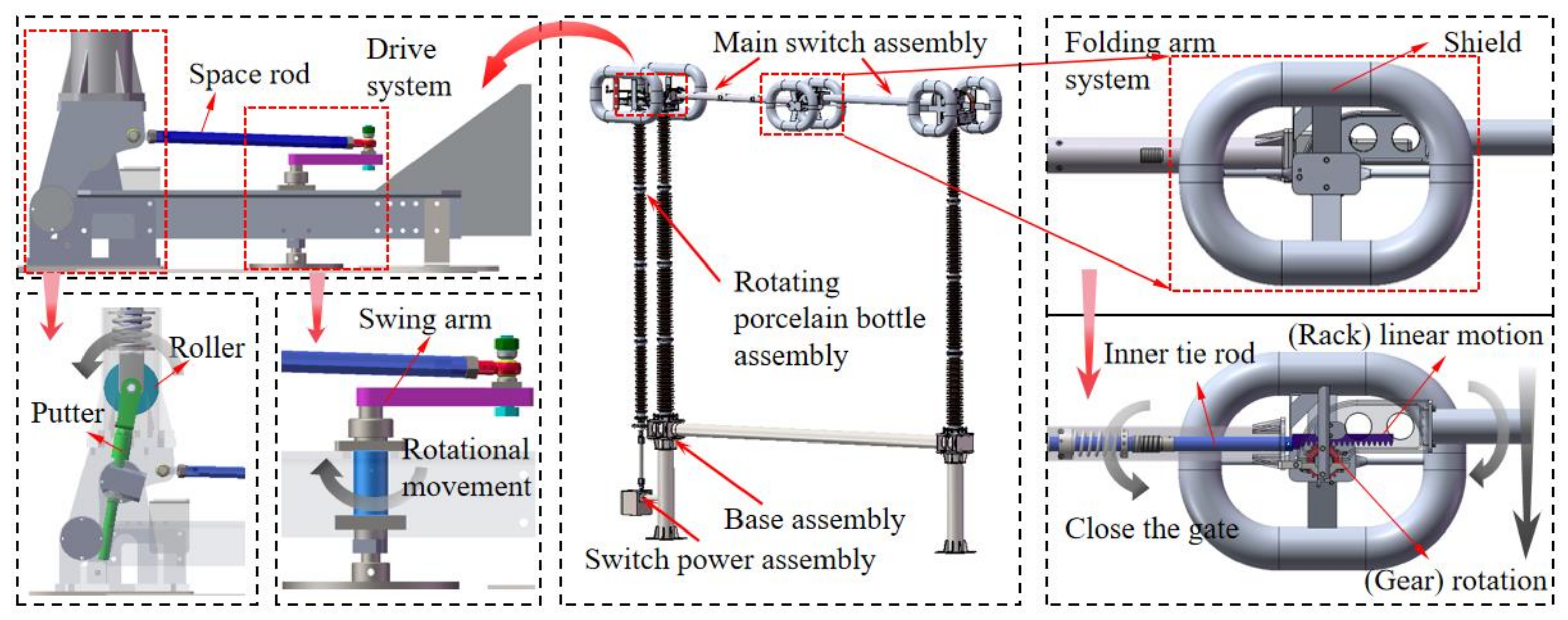
The main switch of disconnector mainly includes drive system and folding arm system. The mathematical models of the two parts are established respectively, and the geometric relationship between the components is deduced, which provides a theoretical basis for the later optimization design.

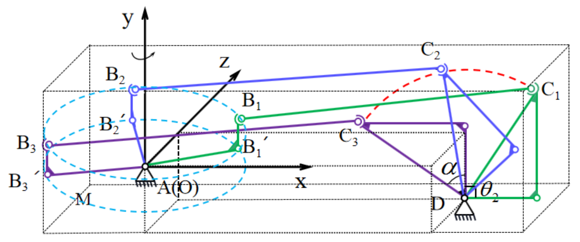
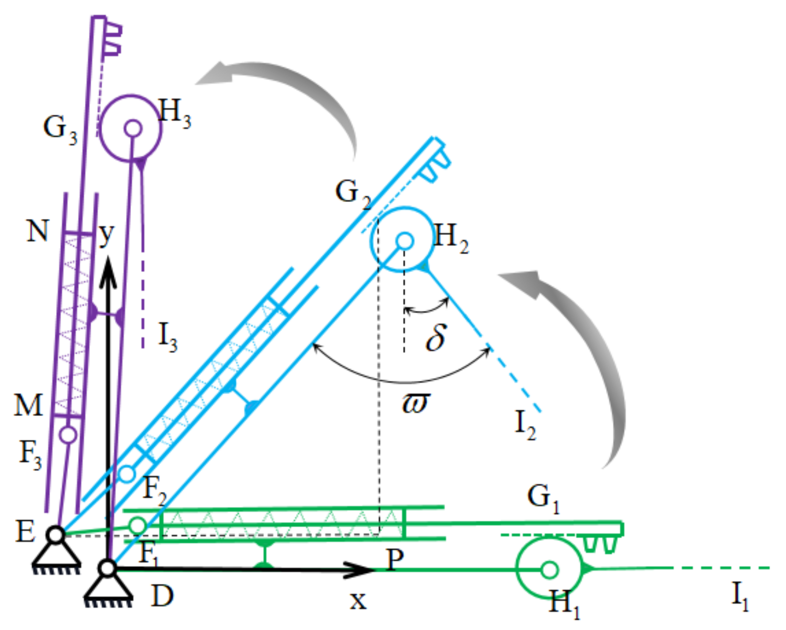
The mathematical analysis model of the drive system is shown in Figure 3. The coordinate system O-xyz is established at O (0,0,0), where point A coincides with point O, Subscript 1 represents the initial position of the spatial four-bar, subscript 2 represents a certain position in the middle of the spatial four-bar, and subscript 3 represents the end position of the spatial four-bar. In the Figure 3, A and D are the fixed frame, AB′ is the rotating arm, and it rotates in the M plane around point A with Oy as the axis; AB′ and BB′ are a whole, moving with the movement of AB′; BC is the space rod, B and C are the ball pairs; the CD is a frame that rotates around point D. Suppose the turning angle of AB′ is $\phi$, the included angle of frame D is $\theta$, and the angle between swing arm and space rod is $\epsilon$. In this paper, the coordinates of all points are expressed as ${\left[x,y,z\right]}^T$in the form of column vector, and the name of the point is expressed by subscript (for example, the coordinate of point D is ${\left[x_D,y_D,z_D\right]}^T$). Let AB′ = L₁, BB′ = L₂, BC = L₃, CD = L₄.

(1)

The value of $\phi$

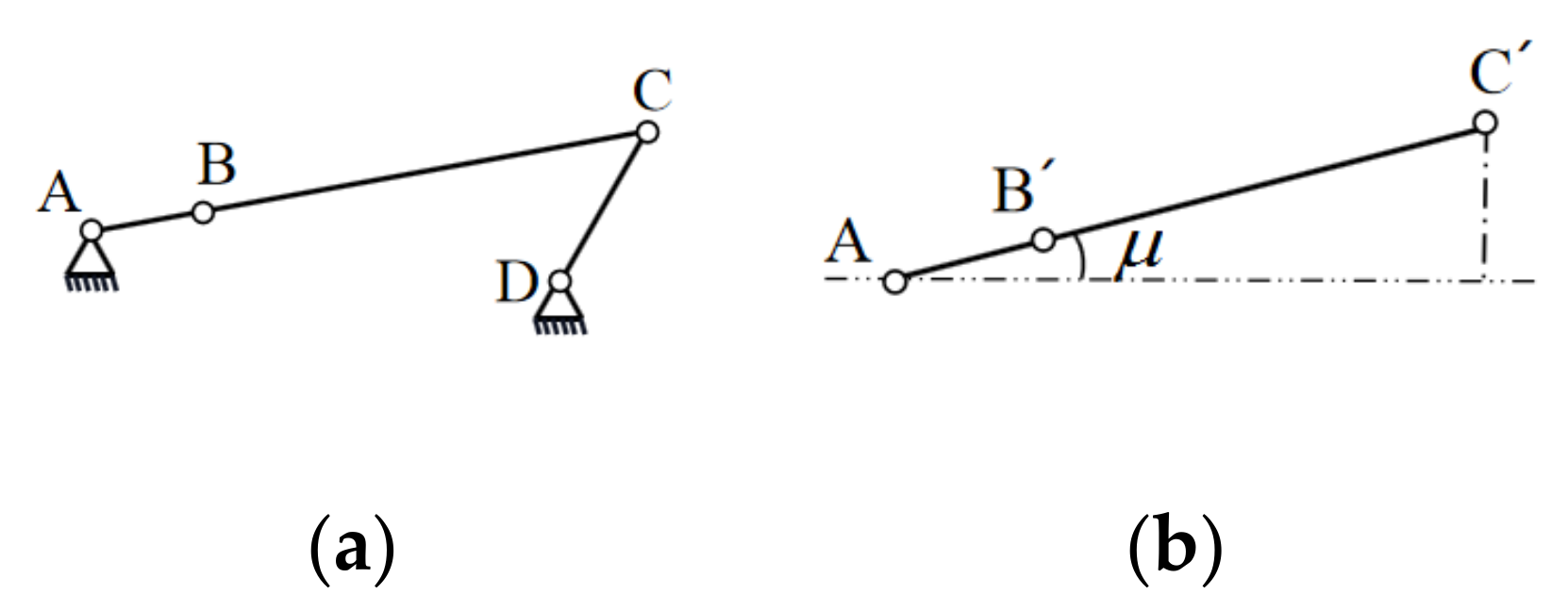
In order to ensure the stability of the mechanism when opening and closing the disconnector, it is necessary to ensure that the swing arm AB′ and the pull rod BC are at the dead center position relative to the component CD. The schematic diagram of the four-bar mechanism in the closed state is shown in Figure 4. The projection of the swing arm and the pull rod on the rotating plane of the swing arm are on the same straight line. Assuming that the angle between the swing arm and the horizontal axis of the base is $\mu$, according to Figure 4b, we can get:

$$\mu =\mathit{arctan}\frac{z_{C_1}-z_A}{x_{C_1}-x_A}$$

(2)

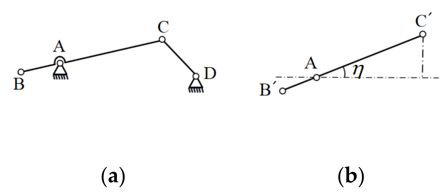
The schematic diagram of the four-bar mechanism in the open state is shown in Figure 5. Since the rod length of the space rod BC is much larger than the length of BB′, the length of BB′ is ignored and it is approximately regarded as the swing arm and the draw rod parallel. The angle between the horizontal axes of the base is $\eta$, according to Figure 5b, we can get:

$$\eta =\mathit{arctan}\frac{z_{C_3}-z_A}{x_{C_3}-x_A}$$

(3)

Therefore, the value range of the swing arm:

$$0^{°}\le \phi \le {180}^{°}-\mu +\eta$$

(4)

$${\phi }_{max}={180}^{°}-\mathit{arctan}\frac{z_{C_1}-z_A}{x_{C_1}-x_A}+\mathit{arctan}\frac{z_{C_3}-z_A}{x_{C_3}-x_A}$$

(5)

where ${\phi }_{max}$ is the maximum turning angle of swing arm.

(2)

Establish expressions for $\theta$ and $\phi$

When the motor drives AB′ to rotate, the frame CD will rotate with the movement of the multi-link. According to the geometric relationship between the bars in Figure 3, the following equation can be obtained.

The swing arm moves in the M plane, and the coordinate vector of point B′ can be obtained from the coordinate relationship between A and B′:

$${\overrightarrow{R}}_{O{B}^{\prime }}={\overrightarrow{R}}_{OA}+{\mathit{P}}_1\cdot {\mathit{Q}}_1\left(\phi \right)$$

(6)

where

$${\mathit{P}}_1=\left[\begin{array}{cc}{L}_1& 0\\ 0& 0\\ 0& L_1\end{array}\right],{\mathit{Q}}_1\left(\phi \right)=\left[\begin{array}{c}\mathit{cos}\phi \\ \mathit{sin}\phi \end{array}\right]$$

(7)

${\mathit{P}}_1$ and ${\mathit{Q}}_1\left(\phi \right)$ are the relation coefficient matrix and parameter matrix of points A and B′ respectively, ${\overrightarrow{R}}_{OA}$ and ${\overrightarrow{R}}_{O{B}^{\prime }}$ are the coordinate vectors of points A and B′ respectively.

The movement of BB′ is perpendicular to the M plane, then the coordinate vector of point B is:

$${\overrightarrow{R}}_{OB}={\overrightarrow{R}}_{O{B}^{\prime }}+\left[\begin{array}{c}0\\ L_2\\ 0\end{array}\right]$$

(8)

Substituting Equation (6) into Equation (8), we can get:

$${\overrightarrow{R}}_{OB}={\overrightarrow{R}}_{OA}+{\mathit{P}}_1\cdot {\mathit{Q}}_1\left(\phi \right)+\left[\begin{array}{c}0\\ L_2\\ 0\end{array}\right]$$

(9)

In the plane where the frame D rotates, the coordinate vector of point C can be obtained from point D:

$${\overrightarrow{R}}_{OC}={\overrightarrow{R}}_{OD}+{\mathit{P}}_2\cdot {\mathit{Q}}_2\left(\theta \right)$$

(10)

where

$${\mathit{P}}_2=\left[\begin{array}{cc}{L}_4& 0\\ 0& L_4\\ 0& 0\end{array}\right],{\mathit{Q}}_2\left(\theta \right)=\left[\begin{array}{c}\mathit{cos}(\alpha +\theta )\\ \mathit{sin}(\alpha +\theta )\end{array}\right]$$

(11)

${\mathit{P}}_2$ and ${\mathit{Q}}_2\left(\theta \right)$ are the relation coefficient matrix and parameter matrix of points C and D respectively, ${\overrightarrow{R}}_{OC}$ and ${\overrightarrow{R}}_{OD}$ are the coordinate vectors of points C and D respectively.

From the coordinates of B and C, the length of BC rod can be obtained as:

$$L_3=\left|{\overrightarrow{R}}_{OC}-{\overrightarrow{R}}_{OB}\right|$$

(12)

By substituting Equation (9) and Equation (10) into Equation (12), we can get:

$$L_3=\left|\left({\overrightarrow{R}}_{OD}+{\mathit{P}}_2\cdot {\mathit{Q}}_2\left(\theta \right)\right)-\left({\overrightarrow{R}}_{OA}+{\mathit{P}}_1\cdot {\mathit{Q}}_1\left(\phi \right)+\left[\begin{array}{c}0\\ L_2\\ 0\end{array}\right]\right)\right|$$

(13)

It can be seen from Equation (13) that under the condition that the length of each pole is determined, the functional relationship between the angle of the swing arm $\phi$ and the angle of the lower conducting rod $\theta$ can be obtained, where $\theta$ is the implicit function of $\phi$.

$$\overrightarrow{A{B}^{\prime }}\cdot \overrightarrow{BC}=\left|\overrightarrow{A{B}^{\prime }}\right|\cdot \left|\overrightarrow{BC}\right|\cdot \mathit{cos}\overrightarrow{A{B}^{\prime }},\overrightarrow{BC}$$

(14)

where $\overrightarrow{A{B}^{\prime }}={\overrightarrow{R}}_{{OB}^{\prime }}-{\overrightarrow{R}}_{OA}$, $\overrightarrow{BC}={\overrightarrow{R}}_{OC}-{\overrightarrow{R}}_{OB}$.

$$\epsilon =arc\mathit{cos}\frac{\left({\overrightarrow{R}}_{O{B}^{\prime }}-{\overrightarrow{R}}_{OA}\right)\cdot \left({\overrightarrow{R}}_{OC}-{\overrightarrow{R}}_{OB}\right)}{\left|\left({\overrightarrow{R}}_{O{B}^{\prime }}-{\overrightarrow{R}}_{OA}\right)\right|\cdot \left|\left({\overrightarrow{R}}_{OC}-{\overrightarrow{R}}_{OB}\right)\right|}$$

(15)

3.2. Motion Analysis of Folding Arm System

The main switch of disconnector mainly includes drive system and folding arm system. The mathematical models of the two parts are established respectively, and the geometric relationship between the components is deduced, which provides a theoretical basis for the later optimization design.

In order to ensure that the folding arm does not interfere with the frame when closing, the movement diagram of the folding arm system as shown in Figure 6 is established. Establish a coordinate system D-xy at D, where the subscript 1 represents the closing position of the folding arm system, the subscript 2 represents a certain position in the middle of the folding arm system, and the subscript 3 represents the opening position of the folding arm system. The relationship between geometric and motion parameters of the folding arm system is analyzed to provide theoretical guidance for the optimal design of spatial four-bar linkage. Let DE = R, DH = L₅, GH = r, EG = T, the angle between the folding arm is $\varpi$, and the angle between DE and y axis is $\mathsf{\beta }$.

From the geometric relationship of the organization diagram:

$$T=EG=\frac{EP}{\mathit{cos}\theta }$$

(16)

$$EP=L_5\mathit{cos}\theta +R\mathit{sin}\beta -r\mathit{sin}\theta$$

(17)

Substituting Equation (17) into Equation (16), we can get:

$$T=\frac{L_5\mathit{cos}\theta +R\mathit{sin}\beta -r\mathit{sin}\theta }{\mathit{cos}\theta }$$

(18)

In the initial state, the mechanism is in the closed state, and we can get:

$$T_0=L_5+R\mathit{sin}\beta$$

(19)

$$\Delta EG=T_0-T=\left(L_5+R\mathit{sin}\beta \right)-\frac{L_5\mathit{cos}\theta +R\mathit{sin}\beta -r\mathit{sin}\theta }{\mathit{cos}\theta }$$

(20)

Simplified:

$$\Delta EG=\frac{r\mathit{sin}\theta -R\mathit{sin}\beta \left(1-\mathit{cos}\theta \right)}{\mathit{cos}\theta }$$

(21)

The end of the inner rod is a rack, and the upper conducting rod and the gear are the same whole. When the unfolding mechanism moves, under the action of the rack and pinion, the upper conductive rod rotates with the gear. From the motion diagram, we can see that the change of EG is the arc length that the gear has rotated, and we can get:

$${90}^{\circ }-\delta =\frac{\Delta EG}{2\pi r}\cdot {180}^{\circ }$$

(22)

Substituting Equation (21) into Equation (22), we can get:

$$\delta ={90}^{\circ }\cdot \frac{r\left(\pi \mathit{cos}\theta -\mathit{sin}\theta \right)+R\mathit{sin}\beta \left(1-\mathit{cos}\theta \right)}{\pi r\mathit{cos}\theta }$$

(23)

$$\varpi ={90}^{°}-\theta +\delta$$

(24)

Substituting Equation (23) into Equation (24), we can get:

$$\varpi ={90}^{\circ }\cdot \frac{r\mathit{sin}\theta -R\mathit{sin}\beta \left(1-\mathit{cos}\theta \right)}{\pi r\mathit{cos}\theta }-\theta$$

(25)

It can be seen from Equation (25) that during the operation of the disconnector, the included angle of the folding arm is related to the distance between the frame D and E, the radius of the gear, the included angle between DE and the vertical line, and the angle of the lower conducting rod. In order to avoid interference to the base when the folding arm system is opened, it is necessary to limit the angle of the folding arm so that the angle range of the lower conductive rod can be obtained.

Based on the analysis of the mathematical model of the drive system and the folding arm system, the statistical table of the hard point statistics of disconnector and the expression of the relationship between the parameters can be obtained (

Table 1. Hard point statistics of disconnector.

Name	Point	Definition
The center point of the rotating shaft of the swing arm	A($0,0,0$)	The coordinate value does not change
Turning point of the swing arm	B′ ($L_1\mathit{cos}\phi$, 0, $L_1\mathit{sin}\phi$)	To be optimized
Front ball point of space rod	B ($L_1\mathit{cos}\phi$, $L_2$, $L_1\mathit{sin}\phi$)	To be optimized
Rear ball point of space rod	C ($x_D+L_4\mathit{cos}(\alpha +\theta )$, $y_D+L_4\mathit{sin}(\alpha +\theta )$, $z_D$)	To be optimized
Rack point	D ($x_D$, $y_D$, $z_D$)	The coordinate value does not change
Rack point	E ($x_D-R\mathit{sin}\beta$, $y_D+R\mathit{cos}\beta$, $z_D$)	The coordinate value does not change

), which provides a theoretical basis for the optimization of the parametric prototype model and design model.

4. Simulation and Verification of Disconnector

4.1. Simulation Analysis of the Disconnector

According to the design drawing of GW17 type disconnector, the base, spatial four-bar, upper and lower conductive rod, inner pull rod, gear rack and other components are established in SolidWorks. Finally, the components are assembled according to the position relationship shown in Figure 2 to form the overall assembly of main switch disconnector [24].

After the model is imported into ADAMS, the motion constraints are added according to the motion relationship among the components, and the solid model of GW17 disconnector is established as shown in Figure 7. According to the actual operation requirements, the opening and closing driving process is set: the whole opening and closing process is completed for 20 s, and closing is the reverse operation of opening; during operation, 1 s is accelerated, 2–9 s is uniform, and 10 s is decelerated. The rotation direction is counter clockwise when opening and clockwise when closing.

The initial parameters of the selected product are shown in

Table 2. Initial parameters.

Symbol	Numerical Value	Symbol	Numerical Value
L1	230 mm	$\alpha$	62.5°
L2	65 mm	$\beta$	17.4°
L3	915 mm	R	185 mm
L4	363 mm	r	100 mm

, where $\alpha$ is the included angle of the tripod at the frame D, $\beta$ is the included angle between frame D and E and the vertical line, R is the distance between frame D and E, and r is the radius of the gear.

The dynamic analysis of the opening and closing process is carried out, and the change curves of $\phi$, ${\theta }_c$, $\varpi$, $\epsilon$, and $F_B$ are obtained, as shown in Figure 8. Where${\theta }_{\mathrm{c}}$ is the minimum complementary angle of the lower conducting rod rotation angle, $F_B$ is the force on the ball pair.

When the disconnector is opened, the swing arm moves according to the driving function, with the maximum angle of 180°, and the lower conductive rod rises accordingly. After the disconnector opened, ${\theta }_{min }$ is 6.9°, ${\varpi }_{min}$ is 7.2°, and ${\epsilon }_{min }$ is 7.8°. At the end of opening operation and the beginning of closing, the buffer spring connected with the inner tie rod in the lower conducting rod collided with the outer rigid cylinder. At the same time, due to the friction of the ball pairs at both ends of the space rod, the force of the ball pair is unstable. The maximum force here is 1.4 × 10⁵ N. The analysis shows that the angle of the folding arm of the disconnector is large, the center of gravity of the folding arm system deviates from the direction of the transmission base, and the space rod will receive greater tension, and the space rod is a slender rod, which is prone to fracture. The ball pairs at both ends of the tie rod are worn seriously, which can easily cause mechanical failure. Therefore, it is necessary to optimize the spatial four-bar linkage to make the disconnector more stable and reliable during operation.

Where ${\epsilon }_{min }$ is the minimum included angle between the swing arm and the tie rod, ${\varpi }_{min}$ is the minimum included angle of the folding arm.

4.2. Simulation Result Verification

In order to verify the reliability of the simulation results, it is necessary to test the mechanical characteristics and kinematic characteristics during the opening and closing process, and compare with the simulation results. In this paper, an experimental platform for the GW17-800 high-voltage disconnecting switch was built, and test experiments are carried out. The magneto-sensitive angular displacement sensor is used to measure the angle change. Figure 9 shows the installation position of the angular displacement sensor when measuring $\theta$ and $\varpi$. Carry out opening and closing operations, and record the data with data acquisition instrument.

Table 3. Experimental test data.

Serial Number	First Group (°)		Second Group (°)		Third Group (°)
	${\mathit{\phi }}_{\mathit{m}\mathit{a}\mathit{x}}$	${\mathit{\varpi }}_{\mathit{m}\mathit{i}\mathit{n}}$	${\mathit{\phi }}_{\mathit{m}\mathit{a}\mathit{x}}$	${\mathit{\varpi }}_{\mathit{m}\mathit{i}\mathit{n}}$	${\mathit{\phi }}_{\mathit{m}\mathit{a}\mathit{x}}$	${\mathit{\varpi }}_{\mathit{m}\mathit{i}\mathit{n}}$
1	177.488	5.584	178.2	5.692	176.804	5.674
2	177.596	5.818	177.84	5.8	176.768	5.422
3	177.596	5.854	176.84	5.584	176.544	5.764
4	177.812	5.818	176.84	5.764	176.824	5.8
5	177.812	5.386	177.2	5.764	176.272	5.62
6	177.408	5.206	177.272	5.64	176.832	5.584
7	177.64	5.782	177.2	5.656	176.912	5.368
8	177.76	5.53	177.84	5.8	176.824	5.68
Average	177.64	5.62	177.0	5.71	176.85	5.61

extracts the maximum swing arm angle and the minimum folding arm angle of the three sets of experimental test data. The analysis shows that in the 24 opening and closing processes, the change of the maximum arm angle does not exceed 1.5°, with an error of 0.83%, and the average difference of the three groups does not exceed 1°, with an error of 0.55. The change does not exceed 1°, the error is 0.55%, the average difference of the three groups does not exceed 0.5°, the error is 0.23%. Figure 10 shows the comparison between the simulation and test data of $\theta$ and $\varpi$. It can be seen from the Figure 10 that the trend of simulation data and test data are consistent. Regarding $\theta$ as the input value, and $\varpi$ as the output value, the input and output of the simulation operation can match the input and output of the actual operation, which shows that the simulation model and various parameter settings are relatively reasonable and can correctly reflect the actual operation.

5. Optimal Design and Analysis of Drive System

5.1. Establish Optimization Model

5.1.1. Design Variable

Select design parameters L₁, L₂, L₃, $\phi$as design variables, expressed as:

$$X=\left[x_1,x_2,x_3,x_4\right]$$

(26)

The design variables x₁, x₂, x₃, x₄ are design parameters L₁, L₂, L₃, $\phi$respectively, and the range of design parameters $\theta$, $\epsilon$ and $\varpi$ are constraints. As shown in Figure 11, in the actual engineering design, the end of the swing arm AB′ is a variable-length cogging structure, which is convenient for adjusting the spatial four-bar linkage, and can move 20 mm to the left and right. Therefore, the upper and lower limits of other design variables can be inferred according to the boundary value of the design variable L₁. The initial value and the boundary value of the constraint conditions are shown in

Table 4. Boundary values of design variables and constraints.

Design Variable	Initial Value	Lower Limit	Upper Limit	Constraint Condition	Lower Limit	Upper Limit
L1/mm	230	210	250	$\theta$/°	0	90
L2/mm	65	55	75	$\epsilon$/°	0	180
L3/mm	915	880	940	$\varpi$/°	0	180
$\phi$/°	180	180	190

.

5.1.2. Objective Function

To ensure the stability during opening and closing, it is necessary to make the structure more compact after opening the switch under the condition of meeting the working requirements, especially the rising angle $\theta$ of the lower conducting rod as large as possible, so as to improve the stability of equipment operation. Take the rising angle $\theta$ of the lower conducting rod as the target object, as shown in Equation (27):

$$f\left(X\right)=mean\left[\theta \left(x_1,x_2,x_3,x_4\right)\right]$$

(27)

Then establish the objective function:

$$f\left(X\right)=min\left[\theta \left(x_1,x_2,x_3,x_4\right)\right]$$

(28)

5.1.3. Constraint Condition

The constraints mainly include the size limitation of the connecting rod and the interference between the conductive rod and the frame. The limiting conditions of connecting rod size include the boundary value of design variables and the maximum angle of the swing arm; the interference between the lower conducting rod and the frame is mainly due to the angle between the folding arm is not too small. The constraints can be described as follows:

•          $s.t.$
•          $g_j: x_{jl}\le x_j\le x_{ju}\left(j=1\sim 4\right)$
•          $g_5:-{\epsilon }_{min}$
•          $g_6:-{\theta }_c\le 0^{\circ }$

$$g_7:-{\varpi }_{min}$$

(29)

where$x_{jl }$ and $x_{ju}$ are the lower and upper limits of the design variables.

5.2. Optimization Design Based on ADAMS

ADAMS is a multi-body dynamics analysis software, which integrates modeling, calculation and post-processing. Users can simulate the various movements of the mechanical system, and carry out kinematics and dynamics analysis, observe the operation condition under different conditions, and get the optimal solution [25].

5.2.1. Parametric Virtual Prototype Model

The four-bar linkage mechanism of the disconnector is parameterized. The coordinates of key points are expressed by design parameters, and the geometry is described by the key points after parameterization [26]. The parameterized coordinates of the initial positions of the five key points are shown in

Table 5. Parameterized coordinates of the initial positions of key points.

Point	X	Y	Z
A	0	0	0
B′	$L_1\mathit{cos}\phi$	0	$L_1\mathit{sin}\phi$
B	$L_1\mathit{cos}\phi$	$L_2$	$L_1\mathit{sin}\phi$
C	$x_D+L_4\mathit{cos}(\alpha +\theta )$	$y_D+L_4\mathit{sin}(\alpha +\theta )$	$z_D$
D	$x_D$	$y_D$	$z_D$

, where L₁, L₂, L₃, L₄, $\alpha$,$\theta$, $\phi$, $\epsilon$, $x_D$, $y_D$, $z_D$ are design parameter.

5.2.2. Model Design Research

Within the variation range, the values of AB′, BB′, BC are changed to observe the change of the objective function, which can provide reference for the later optimization design. Figure 12a,b are the curves of the change of $\theta$ with AB’ and BB’ respectively, and Figure 12c is the curve of ${\theta }_{max}$ changing with AB′ and BB′. It can be seen from the Figure 12 that when AB’ is 215 mm,${\theta }_{max}$ is 75.7°; when AB’ is 245 mm, ${\theta }_{max}$ is 95.6°. Within the value range, ${\theta }_{max}$ increased by 19.9°; when BB′ is 57 mm, ${\theta }_{max }$ is 84.5°; when BB′ is 75 mm, ${\theta }_{max }$ is 95.6°. Within the value range, ${\theta }_{max}$ increased by 0.9°. The analysis shows that the length of AB′ and BC (the changing trend of $\theta$ with BC is the same as AB′) has a greater influence on $\theta$, and BB′ has a smaller influence on $\theta$.

5.2.3. Optimization Based On ADAMS

The design variables, objective functions and constraint functions are as shown above. The constraint functions are converted into ADAMS script language, and the OPTDES-GRG algorithm is used for optimization, which has good convergence [25]. The value and change rate of the design variables before and after optimization are shown in

Table 6. Particle swarm optimization conditions setting.

Particle Dimension	Number of Particles	$\mathbf{Learning}\mathbf{Factor} {\mathit{c}}_1$$,{\mathit{c}}_2$	Inertia Weight	Maximum Speed	Maximum Number of Iterations
5	50	0.8	0.5	0.1	100

. The change curves of ${\theta }_c$, $\varpi$, $\epsilon$ and $F_B$ before and after optimization are derived from the post-processing, as shown in Figure 13.

After optimization, ${\theta }_c$ becomes 2.2°, which is 68.1% less than before optimization; ${\varpi }_{min}$ is 0.8°, which is 87.1% less than before optimization; ${\epsilon }_{min }$ is 1.4°, which is 82.0% less than before optimization; the maximum $F_B$ is 9.0 × 10⁴ N, which is 35.7% less than before optimization. By analyzing the optimized data, the center of gravity of the mechanism is close to the base direction after the optimized disconnector is opened, and the swing arm and tie rod of the spatial four-bar linkage are close to the dead point, which greatly reduces the wear of the ball pair and ensures the long-term and stable operation of the mechanism.

5.3. Optimal Design Based on PSO

5.3.1. PSO Algorithm

Particle swarm optimization algorithm is used to imitate the foraging behavior of birds and use swarm intelligence to search for better solutions. In the algorithm, the position information of each individual bird represents a particle, and the position information of each particle indicates that the particle is a potential solution to the target problem. Finally, the value of these solutions can be judged by the objective function. Each particle has two attributes: speed and position. Speed represents information about the speed and direction of a particle’s movement, and position represents coordinates of the position of the particle. The optimal solution among all the solutions obtained by the particle in the search process is called the individual extreme value, which corresponds to the global optimum solution [26]. Figure 14 shows the flow chart of particle swarm optimization algorithm.

In the last 30 years, many new particle swarm optimization algorithms have been developed and applied to solve problems. Tanweer et al. [27] proposed a new particle swarm optimization algorithm, which is called the self-tuning particle swarm optimization (SRPSO) algorithm. The SRPSO algorithm can converge faster and provide better solutions to problems in most cases. Lynn et al. [28] proposed a comprehensive learning particle swarm optimization algorithm called “Heterogeneous Comprehensive Learning Particle Swarm Optimization” (HCLPSO), which is more exploratory and developmental. Xu et al. [29] proposed an accelerated two-stage particle swarm optimization (ATPSO) with the same efficiency as K-means particle swarm optimization (KPSO). Compared with Pareto based multi-objective PSO, ATPSO can detect clustering more accurately and quickly through the proposed two-stage search. This paper adopts the multi-objective particle swarm optimization algorithm, which has the advantages of simple implementation, efficient search and fast convergence, and has been widely used in engineering practice.

Assuming that the dimension of particles in the population is $\mathsf{\Lambda }$ and the number of particles is $\mathsf{{\rm Y}}$, the velocity and position of the k-th particle in the t-th iteration of the population can be expressed as:

$$v_k\left(t\right)=\left(v_{k,1}\left(t\right),v_{k,2}\left(t\right),\dots ,v_{k,D}\left(t\right)\right)$$

(30)

$$x_k\left(t\right)=\left(x_{k,1}\left(t\right),x_{k,2}\left(t\right),\dots ,x_{k,D}\left(t\right)\right)$$

(31)

The velocity and position of the k-th particle of the population in the (t + 1)-th iteration can be expressed as:

$$v_k\left(t+1\right)=\omega v_k\left(t\right)+c_1{r}_1\left(p_{best}-x_k\left(t\right)\right)+c_2{r}_2\left(g_{best}-x_k\left(t\right)\right)$$

(32)

$$x_k\left(t+1\right)=x_k\left(t\right)+v_k\left(t+1\right)$$

(33)

where t is the current evolutionary algebra, $p_{best}$ is the local optimal solution, $g_{best}$ is the global optimal solution, $\omega$ is the value of the inertia weight, $c_1$ and $c_2$ are learning factor (non-negative numbers),$r_1$ and $r_2$ are two random values of interval [0,1](0,1) [30].

5.3.2. Optimization Based On PSO

Since the optimization content of the two methods is the same, the setting of design variables, objective functions, and constraint functions are the same as Section 5.1. The condition settings of the particle swarm optimization model are shown in Table 6. The procedure of the particle swarm optimization algorithm used in this article is shown in Algorithm A1.

Substituting the algorithm into MATLAB for experimentation shows when the particle swarm optimization algorithm iterates for the 26th time, the objective function value quickly drops to a very low level. After the iteration, the objective function value gradually tends to be flat, indicating that the particle swarm algorithm has converged. The value and change rate of the design variables before and after optimization are shown in

Table 7. Parameters before and after optimization based on ADAMS and PSO algorithm.

Design Parameters	Before Optimization	After ADAMS Optimization	Rate of Change/%	After PSO Algorithm Optimization	Rate of Change/%
L1/mm	230	237	3	240	4.3
L2/mm	65	74	13.8	74	13.8
L3/mm	915	905	−1.1	900	−1.5
${\phi }_{max}$/°	180	184	2.2	184.2	2.2
${\theta }_c$/°	6.9	2.2	−68.1	2.0	−71.0
${\varpi }_{\min }$/°	7.2	0.8	−87.1	0.7	−88.7
${\epsilon }_{min}$/°	7.8	1.4	−82.0	1.3	−83.3

. The change curves of ${\theta }_c$, $\varpi$, $\epsilon$ and $F_B$ before and after optimization are shown in Figure 15.

5.4. Comparative Analysis of Optimization Results

As shown in Table 7, the length of swing arm AB′ after ADAMS optimization is increased by 7 mm, which is 3% more than that before optimization. After optimization by PSO algorithm, the length of swing arm AB′ is increased by 10 mm, which is 4.3% higher than that before optimization, and the optimized length is within the allowable range. After optimization by ADAMS and PSO, the connecting rod BB′ is increased by 9 mm, which is 13.8% more than before optimization, and ${\phi }_{max}$ is increased by 2.2% compared to before optimization, which ensures that the tie rod is parallel to the swing arm and close to the dead point when the brake is opened. After optimization by ADAMS, the space rod BC is reduced by 10 mm, which is 1.1% less than before optimization; after optimization by PSO algorithm, the space rod BC is reduced by 14 mm, which is 1.5% less than before optimization, which achieves a lightweight structure and makes the tie rod less likely to be damaged.

As shown in Figure 15, the design parameters $\theta$, $\epsilon$, and $\varpi$ after optimization by the ADAMS method and the PSO method have the same changing trend. After PSO algorithm optimization, ${\theta }_c$ is 2.0° and decreases by 71.0%; ${\varpi }_{min}$ is 0.7° and decreases by 88.7%; ${\epsilon }_{min }$ is 1.3° and decreases by 83.3%; the maximum $F_B$ is 9.0 × 10⁴ N and decreases by 35.7%.

By comparison, the optimization results of the two methods are very close, which verifies the reliability of the optimization results. The result of PSO optimization is slightly better than that of ADAMS, and the swing arm length AB′ after PSO optimization is still within the variable range. Although it is increased, the influence on the opening and closing movement can be ignored. Compared with the results of ADAMS optimization, the length of the space rod is reduced by 4 mm, ${\theta }_c$ is reduced by 2.9%, ${\varpi }_{min}$ is reduced by 1.6%, and ${\epsilon }_{min }$ is reduced by 1.3%.and the performance is better.

6. Physical Prototype Experiment

Based on the previous analysis, this paper conducts an experimental study on the performance of the physical model after the optimization of the GW17-800 high-voltage disconnecting switch. The swing arm was adjusted to 240 mm, the connecting vertical rod to 74 mm, and the space rod to 900 mm. After adjusting the length of each rod, it was verified on the experimental platform shown in Figure 16.

The angular displacement sensor was installed according to the position shown in Figure 10, performed the opening and closing movement, and the collected data compared with the simulation optimization results. The comparison result is shown in

Table 8. Comparison of simulation and experimental optimization results.

Parameter	Simulation	Experiment	Error/%
${\phi }_{max}$/°	184.2	178.6	3.1
$\theta$/°	88	89.5	1.7
$\varpi$/°	179.3	176.8	1.4

. The experimentally measured ${\phi }_{max}$ is 178.6°, and the error from the simulation result is 3.1%; $\theta$ is 89.5°, and the error is 1.7%; $\varpi$ is 176.8°, and the error is 1.4%. The error between simulation and experiment is small, which verifies the effectiveness of the optimization results, and the performance of the optimized results is good, achieving the goal of optimization.

7. Conclusions

This paper takes the GW17 high-voltage disconnecting switch as the research object. First, the optimization model of the disconnector is established, and the spatial four-bar linkage mechanism is optimized by using ADAMS and PSO algorithm. Then, an experimental platform is built to verify the simulation results and optimize the correctness of the results.

After optimization, the length of the swing arm is 240 mm, the length of the vertical rod is 74mm, and the length of the space rod is 900 mm. The minimum corner angle of the lower conductive rod is reduced by 71.0%, and the minimum folding arm angle is reduced by 88.7%. The angle of the tie rod is reduced by 83.3%, the angle between the swing arm and space rod is reduced by 83.3% and the maximum force of the ball pair has been reduced by 35.7%.

When the optimized disconnector is in operation, the space rod is closer to the dead center position, the opening and closing of the folding arm system is more in place, the wear is reduced, the light weight is realized, and improving the stability and reliability of equipment operation. In this paper, only the rigid body research is carried out on the high-voltage disconnecting switch, and further rigid-flexible coupling analysis of the model is needed.