A Markov-Switching VSTOXX Trading Algorithm for Enhancing EUR Stock Portfolio Performance

Abstract

In the present paper, we test the benefit of using Markov-Switching models and volatility futures diversification in a Euro-based stock portfolio. With weekly data of the Eurostoxx 50 (ESTOXX50) stock index, we forecasted the smoothed regime-specific probabilities at T + 1 and used them as the weighting method of a diversified portfolio in ESTOXX50 and ESTOSS50 volatility index (VSTOXX) futures. With the estimated smoothed probabilities from 9 July 2009 to 29 September 2020, we simulated the performance of three theoretical investors who paid different trading costs and invested in ESTOXX50 during calm periods (low volatility regime) or VSTOXX futures and the three-month German treasury bills in distressed or highly distressed periods (high and extreme volatility regimes). Our results suggest that diversification benefits hold in the short-term, but if a given investor manages a two-asset portfolio with ESTOXX50 and our simulated portfolios, the stock portfolio’s performance is enhanced significantly, in the long term, with the presence of trading costs. These results are of use to practitioners for algorithmic and active trading applications in ESTOXX50 ETFs and VSTOXX futures.

1. Introduction

Volatility futures are a type of security whose development started in the decade of the 1990s [1,2,3] with the inception of Volatility indexes (VSTOXX henceforth). Volatility is an essential, well-known, and established concept in Finance, Financial economics, and the financial industry. The term is a cornerstone in security asset pricing models and the rational (quantitative) investment selection process. The focus of the present paper is not to make a formal description of the role of volatility, proxied with either the standard deviation $\sigma$ or the variance ${\sigma }^2$ of a given security’s return time series. It must be mentioned that the expected return of that given security or investment is closely related (and determined) by the risk or volatility level.

Financial derivatives have had a special interest in asset pricing since their ancient origins in the Ancient Greek and Japanese cultures [4,5,6], or their more recent origins during the development of the Dutch, French, or English agricultural exchanges from the 17th to 19th centuries.

This led to the development of the traded European options contracts with a given exercise price $K$ settled at a future exchange date $T$. These options’ values are determined with the spot or actual price $S_t$ of a stock (or other underlying point) in the market with which a premium $C_t$is paid by the option’s buyer. On the other hand, the issuer of this theoretical option must deliver the agreed stock at the agreed price even if $S_t>K$ at $T$.

This option valuation rationale allowed an interesting development of other derivatives markets such as those of the volatility level with which these options are evaluated.

For the specific case of option premiums (especially in agricultural commodities), the mathematical interest for a proper valuation model started in the 19th century and motivated the first option valuation models [7,8]. These were based on the well-accepted valuation rationale presented in the seminal works of Markowitz [9,10] and Tobin [11]. Given the need for wider and more liquid options and futures markets, Black, Scholes, and Merton [12,13] demonstrated a valuation method for European options, that is, options that, contrary to other types such as American options, cannot be exercised (liquidated) in a time $t<T$. This led them to the next respective expressions for the valuation of a “call” or buy option ($C_t,$ as in the previous example) and a “put” or sell option ($P_t$):

$$C_t=S_t·N\left(d_1\right)-e^{-rf\left(T-t\right)}·K·N\left(d_2\right)$$

(1)

$$P_t=C_t-S_t+e^{-rf\left(T-t\right)}·K$$

(2)

In the two previous expressions, $rf$ is the risk-free asset rate. It is an interest rate that represents a low-risk investment for the holder in the shortest available investment period; that is, it corresponds to the rate of return paid by the shortest redemption period of the available government money-market securities. For the specific case of the U.S., the risk-free rate is the three-month U.S. Treasury bill (TBILL), and for the case of Europe and this paper, it is the three-month German treasury bill (Bundes).

Additionally, in those equations, $N(·)$ is the accumulated Gaussian or normal probability density function (pdf) of parameters $d_1$ and $d_2$. These are estimated as follows:

$$d_1=\frac{\ln \frac{s_t}{K}+\left(rf+0.5·{\sigma }^2\right)\left(T-t\right)}{\sigma \left(T-t\right)}$$

(3)

$$d_2=\frac{\ln \frac{s_t}{K}+\left(rf-0.5·{\sigma }^2\right)\left(T-t\right)}{\sigma \left(T-t\right)}$$

(4)

These two terms represent the standardized values of the likelihood that the valuated option ends, at $T$, at the money ($s_t>K$ in (3), or $s_t<K$ in (4)) or out of the money ($s_t<K$, or $s_t>K$), respectively.

The Black-Scholes-Merton option valuation model of (1) and (2) is a cornerstone that led to the development of the interbank (over-the-counter, or OTC) and well-known, established option markets such as the Chicago Board of Options Exchange (CBOE), which is now part of the Chicago Mercantile Exchange (CME), and the Deutsche Terminbörse (currently part of the Eurex exchange). These last two established markets experienced an important trading volume that led them to be the most liquid markets in the world, with a combined turnover of almost 100 million options in open interest as of January 2021 [14].

From the input parameters in (3) and (4), a special option price sensitivity plays an important role in options pricing. This sensitivity is that related to the option’s price change, given the change of the volatility level $\sigma$. A sensitivity known as vega ($\nu$) is calculated as follows:

$$\nu =\frac{\partial C_t}{\partial \sigma }=\frac{\partial P_t}{\partial \sigma }=K{e}^{-rf\left(T-t\right)}N\prime \left(d_2\right)\sqrt{T-t}$$

(5)

This sensitivity plays an important role in banks and brokerage houses’ option trading books and current positions, and, as will be mentioned later, it developed the need for volatility indexes. The related volatility $\sigma$ level in (1)–(5) is a fundamental parameter that determines the option’s market price. Given this, a current option position could have important price fluctuations if the volatility value $\sigma$ shows a significant change. Based on this rationale, the options volatility level ($\sigma$) becomes a potential underlying financial factor to be hedged, along with the option’s underlying asset price $S_t$.

To solve the need of volatility hedging in option positions, Grünblicher and Longstaff [15] were the first authors to discuss this possibility and the need for implied volatility ($\widehat{\sigma }$). The concept of implied volatility $\widehat{\sigma }$ refers to the volatility level necessary in (1) or (2) to reach the put or call market option value. Therefore, in well-established markets such as the Eurex or the CBOE-CME, the put and call options are valued by market participants based on their experience and valuation models that lead to a proper mark-to-model valuation process during trading. Given this, these market prices have an implied market volatility level $\widehat{\sigma }$. Given this implied volatility level, a general implied volatility index (VSTOXX) of currently traded options (puts and calls) could be estimated. These two authors gave the theoretical and mathematical foundations for this possibility.

Thanks to Grünblicer and Logstaff’s work and Brenner and Galai’s [16] proposal, the stochastic process of the volatility $\sigma$ could be modeled. Given the domain of values of volatility ($\sigma \in (0,\infty$)), its value could be proxied as a mean-reverting one, as in the case of the Cox, Ingersoll, and Ross [17] stochastic process of an interest rate or fixed-income security [18,19]. With this rationale for the volatility’s value at $t$ (${\sigma }_t$), Grünblicher and Longstaff proposed the following stochastic process:

$$d{\sigma }_t=\kappa \left({\sigma }_t-\tau \right)d_t+{\sigma }_{{\nu }_t}\sqrt{t}d{Z}_t$$

(6)

In the previous expression, $\tau$ is a long-term volatility value to which the current volatility ${\sigma }_t$ at $t$ converges. $\kappa$ is the rate of convergence; ${\sigma }_{{\nu }_t}$ is the volatility; and $d{Z}_t$ is a Wiener process (Brownian motion).

The development of options market VSTOXX indexes, proposed by Brenner and Galai, led to the development of several volatility derivatives. Based on this, several volatility futures were issued in the CME and the Eurex. The first one was issued in the CBOE-CME in 1993 for the implied volatility (VIX) index of the S&P 500 stock index. In the specific case of the Deutsche Terminbörse (now Eurex), an implied volatility index (VDAX) was issued for the implied volatility of the DAX index options. Later, in 1998, Eurex introduced the Eurostoxx 50 volatility index (VSTOXX) that is the implied volatility index of the Eurostoxx 50 European stock index (ESTOXX50). Based on these European volatility indexes, several futures were issued for the VSTOXX since 2005. Futures were later substituted by a more liquid version of these: the VSTOXX mini-futures. In these, the number of Euros (EUR) to be paid for each VSTOXX point is smaller (EUR 100) than the original futures. This led to more liquid trading positions.

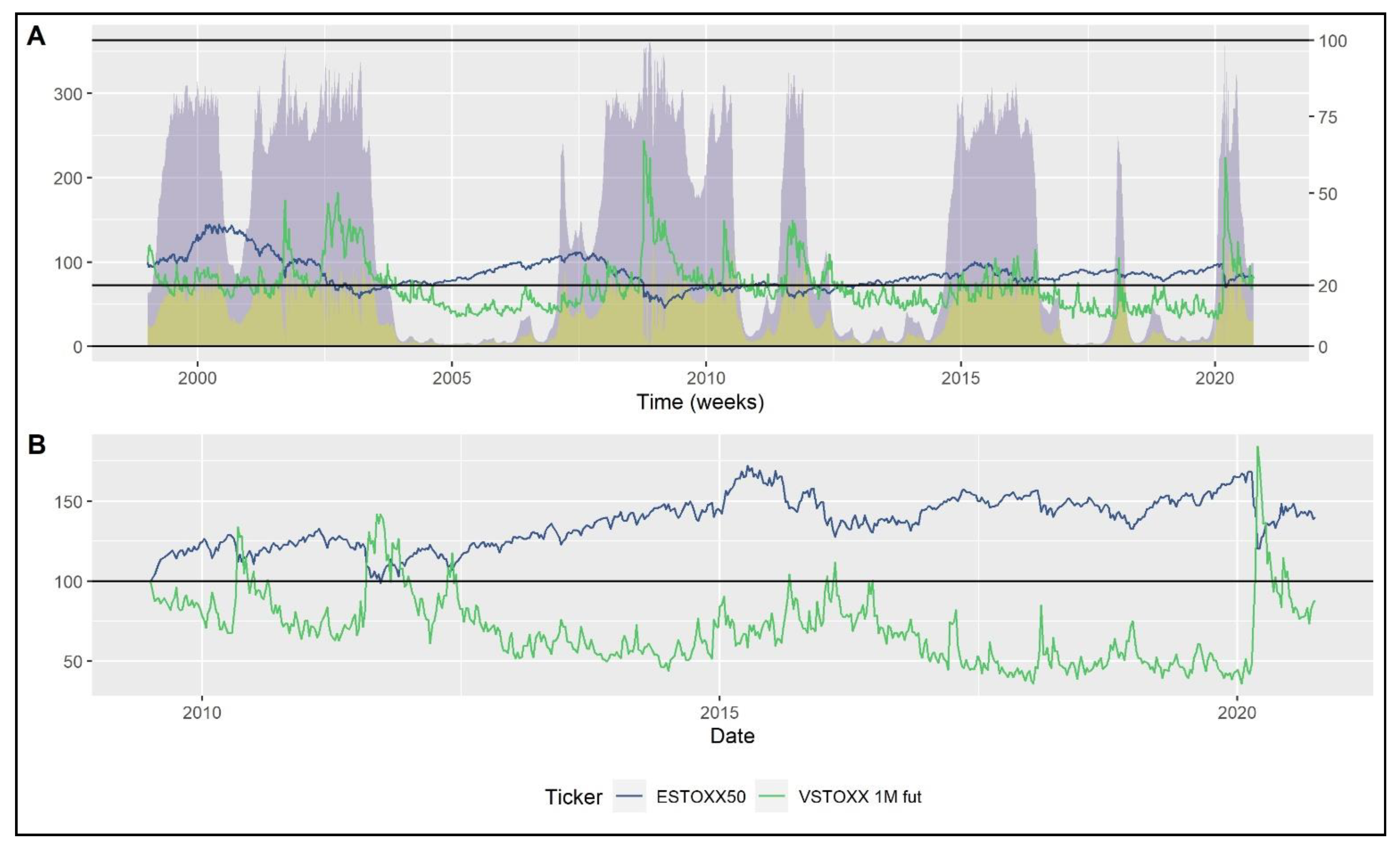
Given the VIX and VSTOXX futures markets development, these were seen as a potential source of diversification in a portfolio. That is, a well-accepted result from portfolio math and management is the fact that, in a highly volatile period, the correlations between assets tend to increase, and the diversification benefits tend to disappear. Given this, it is necessary to incorporate securities that show negative correlations in these periods. A potential solution to this issue remains in volatility futures [20,21,22,23]. This can be noted in panel A of Figure 1.

In that panel, we present the historical 8 August 1999 base 100 weekly value of the Estoxx 50 index (blue line and left axis) against the historical value of the one-month VSTOXX volatility index (green line and right axis). We also present the smoothed probabilities of being in the high ($s=2$) and extreme ($s=3$) volatility regimes (purple and yellow areas, respectively) at $t$. As noted in that panel, when the high or extreme volatility periods are more likely, the ESTOXX50 index tends to fall dramatically and the VSTOXX tends to increase in the same way. This joint behavior suggests that the VSTOXX could be an interesting source of diversification and could be tested in a Euro (EUR) stock index-volatility future portfolio. Given this, our goal is to extend the current and scant literature about the use of volatility indexes for diversification.

Previous works tested the practical benefits of volatility diversification [24,25,26,27] by investing in stocks of the U.S., the Eurozone, or Switzerland and their corresponding local currency bonds (or money markets) or their volatility index futures. In most cases, these authors found diversification benefits; however, they still observed either a utility function value loss or a significant performance impact with the presence of stock trading or future roll-over costs. Some of the most important conclusions of these works concern the impact of roll-over costs plus the negative risk premium of the volatility index’s stochastic process [28], which led the simulated portfolios to underperform against a buy-and-hold stock only strategy. Regarding the conclusions by Alexander, Kapraun, and Korovilas [24,25], volatility index diversification is appropriate only in times of high volatility. Therefore, in times of distress, a portfolio stock diversified with volatility futures is useful only in high volatility regimes.

Based on these conclusions, De la Torre-Torres, Venegas-Martínez, and Martinez-Torre-Enciso [29] tested the benefit of using two- and three-regime Markov-Switching GARCH (MS-GARCH) models to forecast low ($s=1$), high ($s=2$), and extreme ($s=3$) volatility regimes at $t+1$. Additionally, to invest in S&P 500 stock index volatility index (VIX) futures, requires an investment level given with the smoothed probability ${\xi }_{s,t}$ of being in the high (${\xi }_{s=2,t}$) and extreme (${\xi }_{s=3,t}$) volatility regime. They did this by considering the impact of future roll-over and stock trading costs for individual and institutional investors. Their results suggest that there is an improvement in the stock portfolio performance, but this result holds only in the presence of distressed market periods. They also observe that the use of VIX diversification with MS-GARCH models is only useful for institutional investors.

Given those conclusions, we extended the work of De la Torre-Torres, Venegas-Martínez, and Martinez-Torre-Enciso [29] and Alexander, Kapraun, and Korovilas [24,25] to review the performance that a EUR-based stock portfolio would have had, had the portfolio manager used MS-GARCH models in an ESTOXX50-VSTOXX-Bundes portfolio.

Our position is that the use of MS-GARCH models could help to improve the performance against a pure buy-and-hold ESTOXX50 portfolio, that is, against a passively managed portfolio with the ESTOXX50 as the benchmark.

The contributions of our paper, as we will present next, are to extend the review of the benefits of MS-GARCH models in European (VSTOXX) volatility futures. Additionally, we propose an ESTOXX50/ESTOXX50-VSTOXX diversified portfolio management algorithm to enhance the benefits of volatility diversification in the main European markets. Previous works, such as [24,25,26,27], found short-term benefits in volatility futures portfolio diversification. Additionally, ref. [29] found the benefits of using MS-GARCH models to enhance the short-term timing and performance of a U.S. stock/volatility portfolio but failed to propose investment strategies for the long-term. In this paper, we extended these works by the fact that, first, we tested the use of MS-GARCH models for trading decisions in the Eurostoxx 50 stock index and the VSTOXX futures markets. Second, we tested an investment strategy in which a given individual investor could manage a portfolio with two factors or assets: (1) a theoretical Exchange Traded Fund (ETF) that tracked the ESTOXX50 and (2) an ETF that used our simulated MS-GARCH VSTOXX trading algorithm. As we will present next, the results suggest a long-term benefit either for individual or institutional investors. This result holds even with the presence of roll-over future trading costs or the impact of stock trading fees and taxes.

Regarding research and methodology, we tested the use of MS-GARCH models in our simulations because these are widely used to filter and estimate the parameters of an $S$ number of regimes (or states of nature). There are some other interesting proposals such as the Threshold Autoregressive (TAR) or the Self Exciting TAR (SETAR) models of Tong [30,31]. These last models define, for the TAR and the SETAR, respectively, a stochastic process as follows:

$$x_t=\{\begin{array}{c}{\alpha }_1+{\beta }_1·x_{t-p},s_{t-1}<r\\ {\alpha }_2+{\beta }_2·x_{t-p}+{\epsilon }_{2,t},s_{t-1}\ge r\end{array}$$

(7)

$$x_t=\{\begin{array}{c}{\alpha }_1+{\beta }_1·x_{t-p},x_{t-1}<r\\ {\alpha }_2+{\beta }_2·x_{t-p}+{\epsilon }_{2,t},x_{t-1}\ge r\end{array}$$

(8)

The expression in (7) requires the definition of an observable state-determining variable $s_{t-1}$ that provokes a shift in the behavior of $x_t$. This also requires a threshold value $r$. If there is no known state-determining variable, or it is a hidden and unobservable one, Tong proposes the use of the SETAR model in (8). This model suggests that a regime switch occurs, given the indicator rule in (8).

A drawback of (7) and (8) is the need of the proper definition of $s_{t-1}$ and $r$. The estimation results are sensitive to this. On the other hand, and as we will mention in the literature review, Markov-Switching models (MS) and their extension with time-varying standard deviation or volatility (MS-GARCH) do not need the definition of $s_{t-1}$ or $r$. These models assume that the regime shift in $x_t,$ at $t,$ is modeled with a hidden first-order autoregressive Markovian process. That is, the value of regime $s_t$ is modeled at $t$, with a hidden $S$-state Markovian chain, given a transition probability matrix $\Pi$.

From this feature, it is of no need to determine a threshold value $r$ or a regime shifting variable $s_{t-1}$. The changes of regime can be inferred directly from the time series, along with the transition probabilities $\Pi$ and the regime-specific smoothed probability ${\xi }_{s=i,t}$ at $t$. This smoothed probability, contrary to (7) and (8), could be forecasted at $t+p$.

In a similar perspective, there are other interesting techniques such as wavelet analysis, in which the return or risk time series can be analyzed and filtered in a time-frequency space. This means that the fluctuation properties of a return or risk time series can be decomposed into short-term (long frequencies) and long-term (short frequencies) fluctuations. More specifically, they are used to measure the level of integration that return or risk time series have. Some of the main works that test the level of integration between the main world stock markets (by regions) and the VIX index are those of Marfatia [32,33] and Boubaker and Raza [34]. These works test the short-term and long-term link between these markets and this volatility index. They found evidence of high stock market integration in the long term. Even though there are other regimes or structural breaks models such as TAR, SETAR, or wavelets, these fail to infer the number of regimes and to forecast the probability of being in each in future periods ($T+p$). Given this feature, MS and MS-GARCH models will be used herein, leaving the development of other types of models for further research.

Given their assumptions and properties, MS and MS-GARCH were widely used in several Econometric applications, and their use in securities trading decisions is of interest in this paper.

Once we present our aim and motivations for this paper, we structure it as follows: In the next section, we make a literature review of the previous works that motivated the use of MS-GARCH models for volatility futures trading. In the third section, we present our VSTOXX and ESTOXX50 trading algorithms, along with the ones of our long-term portfolio management simulations. In the fourth section, we discuss our results and main findings, and, in the last section, we present our concluding remarks and guidelines for further research.

2. Literature Review

Given the previous introduction, our literature review will be introduced in two parts. We first discuss the previous works that tested the benefits and limitations of volatility futures portfolio diversification. Second, we review the literature that tests the benefits of MS-GARCH models in trading and investment decisions.

The need and potential benefits of volatility futures diversification were primarily suggested in the works of Daigler and Rossi [20], Hafner and Wallmeier [21,35], and Szado [22]. These papers studied the negative correlation of volatility futures and variance swaps with stocks of the SP500 and EUROSTOXX50 stock indexes. Given the recent inception of volatility futures and the option-like profile of variance swaps, the authors found evidence about the benefits of volatility diversification in the 2008 financial distress period. As noted, the short time series given the recent inception of these futures led to results that suggest their benefits. Despite this, the mean-reverting property of variance’s stochastic process in (8) and the impact of roll-over costs (as Alexander, Kapraun and Korovilas [24,25] showed) suggest that volatility diversification has its limitations in the long term. In the specific case of these three previous works, Daigler and Rossi [20] used a Markowitz [9,10] mean-variance portfolio selection of an SP500/VIX portfolio. The results of these three works do not include the impact of future position roll-over costs and stock trading commissions. Given this, we want to extend their work by incorporating this impact in our tests.

In a similar perspective, Dash and Moran [36] tested the benefit of VIX diversification with the performance of hedge funds. In their results, the authors found a negative and asymmetric correlation between these variables, suggesting the potential benefits of VIX diversification. Despite this result, these authors used the VIX index and not the VIX futures that include the impact of roll-over costs.

Two papers that have a close influence on ours and also make a more detailed review of volatility diversification are those of Alexander, Kapraun, and Korovilas [24] and Alexander, Korovilas, and Kapraun [25]. In these two works, the authors take into account the impact of roll-over costs and the mean-reverting property of variance’s stochastic process. By using a mean-variance-minimum variance and a Black-Litterman [37] optimal portfolio selection process, these authors tested a stock/volatility futures strategy in European and U.S. markets. With a preference threshold strategy in which the expected returns induce volatility diversification, the authors found that the benefits of this strategy hold in the short term. On the other hand, in an ex-post test scenario with stock trading fees and roll-over costs, the situation changes. Their results are in line with the work of Bahaji and Aberkane [26], who test the rational utility function maximization benefit (an ex-ante test) of volatility diversification. These three works motivate our paper because we want to test the benefits of stock portfolio diversification with VSTOXX futures, as the use of MS-GARCH models is an extension that we want to test for timing purposes. Why are MS-GARCH models used for timing? Among the main conclusions that Alexander, Korovilas, and Kapraun [25] show is the result that volatility diversification is useful only in the short term and also the result that this diversification works only in high or extreme volatility periods. Given this, we found the use of MS-GARCH models as a potential solution to determine the proper timing for VSTOXX diversification in an ESTOXX50 portfolio.

This rationale was previously tested in the work of De la Torre-Torres, Venegas Martínez, and Martínez-Torre-Enciso [29], and proved useful in the case of U.S. markets, with the simulation of an SP500 stock portfolio, diversified with one-month VIX futures and the use of Gaussian and t-Student MS-GARCH models. In their results, they followed the rationale of SP500/VIX portfolio diversification, but instead of a mean-variance portfolio selection framework, they used the forecast of the smoothed probabilities ${\xi }_{s=i,T+1}$ of MS-GARCH models. More specifically and by following Brooks and Persand’s [38] selection method, they used each regime-specific smoothed probability to determine the investment level, either in the S&P 500, the VIX, or the USTBILL. In their results, these authors found that the use of MS-GARCH models enhances the performance of the simulated portfolios against a buy-and-hold S&P 500 one. Despite this, the authors found that this better performance is only useful in highly distressed periods such as the financial crisis of 2007–2008 or the 2020 COVID-19 pandemic. Also, the authors proved that, given the impact of stock trading and roll-over costs, their MS-GARCH investment algorithm is useful only for Institutional investors. This led them to suggest that it could be implemented for individual investors had they had access to this kind of strategy through an exchange-traded fund (ETF) or similar investment security.

This last paper is also a very important motivation for the present one due to the fact that we extend their test to the European EUROSTOXX50 and VSTOXX futures markets, and due to the fact that we simulate the performance of a portfolio invested in two ETFs: (1) a EUROSTOXX50-Bundes and (2) VSTOX-Bundes portfolio. The purpose is to prove the long-term benefits of VSTOXX portfolio diversification with an MS-GARCH trading algorithm.

Following these last four works, Jung [27] tested the benefit of volatility diversification with three different portfolio selection methods: (1) the option-based portfolio insurance (OBPI) of Rubinstein and Leland [39], (2) a resetting OBPI strategy with a 1% change in the VIX floor exposure for each 10% increase in this index’s value, and (3) a constant proportion portfolio strategy (CPPI) in VIX futures, given in the utility function of Merton’s [40] continuous-time portfolio model. In his results, Jung found the OBPI and resetting models to be very useful in capturing the bullish trend (constant and long time-periods of upward trend movements) in VIX futures. His portfolio insurance strategies also showed potential benefits for diversification. This work motivates our paper in that we tested the use of MS-GARCH models to determine the appropriate proportion or investment level in VSTOXX futures, EURSTOXX50 stock, or the Bundes, given the regime-specific smoothed probability as investment level.

As pointed out previously in our literature review, we are suggesting the use of MS-GARCH models for investment decisions. Markov-Switching (MS) models represent a time-series analysis method suggested primarily by Hamilton [41,42,43]. The rationale of these models is based on the presence of $S-1$ structural breaks in the behavior of the data set, that leads to an $S\in \mathbb{N}$ number of regimes or states of nature. These regimes are unobserved to the analyst, and the stochastic process $r_t$ of a return time series is switching from one state $s_{t-1}=i$at $t-1$ to another $s_t=j$ at $t$. This switching behavior can be inferred from a hidden $s$-state Markovian chain with an $S\times S$ transition probability (${\pi }_{i,j}=P(s_t=j|s_{t-1}=i)$) matrix $\Pi$:

$$\Pi =\left[\begin{array}{ccc}{\pi }_{i,i}& \cdots & {\pi }_{i,j}\\ ⋮& \ddots & ⋮\\ {\pi }_{j,i}& \cdots & {\pi }_{j,j}\end{array}\right]$$

(9)

Given the transition probability matrix $\Pi$, the probability ${\xi }_{s=i,t}$ of being in each regime at $t$ can be filtered and later smoothed (with a method proposed by Kim [44]) from the time-series realization ($r_t$). This is done by using either a Gaussian or t-Student probability density function (pdf):

$${\xi }_{s,t}=\frac{1}{\sqrt{2\pi }{\sigma }_{{\overline{r}}_t,s}}{e}^{-\frac{1}{2}{\left(\frac{r_t-{\overline{r}}_s}{{\sigma }_{{\overline{r}}_t,s}}\right)}^2}$$

(10)

$${\xi }_{s,t}=\frac{\mathsf{\Gamma }\left(\frac{v_s+1}{2}\right)}{\sqrt{\left(v_s-2\right)\pi }\mathsf{\Gamma }\left(\frac{v_s}{2}\right)}{\left(1+\frac{{\left(\frac{r_t-{\overline{r}}_s}{{\sigma }_{{\overline{r}}_t,s}}\right)}^2}{\left(v_s-2\right)}\right)}^{-\frac{v_s+1}{2}}$$

(11)

As noted from (9)–(11), in which ${\nu }_s$ are the regime-specific degrees of freedom, MS models estimate the behavior of the time series according to the switching behavior of each regime $s$. This allows for the estimation of location (${\overline{r}}_s$) and scale (${\sigma }_{{\overline{r}}_t,s}$) parameters for each regime. This means that a mean and a standard deviation for each regime can also be estimated to determine the volatility and expected return if $r_t$ is a security’s time-series (such as stocks). Given this, the parameter set $\mathsf{\theta }=\left\{{\overline{r}}_s,{\sigma }_{{\overline{r}}_t,s},v_s,{\xi }_{s,t},\Pi \right\}$ of MS models could be used to forecast the probability of being in each regime at $T+n$ time-periods as follows:

$${\xi }_{s,T+n}={\Pi }^n·{\xi }_{s=i,T}$$

(12)

Based on these forecasts or the smoothed regime-specific probabilities ${\xi }_{s,t}$ of $\mathsf{\theta }$, Brooks and Persand [38] suggested and proved as true the benefit of using ${\xi }_{s,t}$ as a portfolio weighting method between the U.K. Financial Times FTSE-100 stock index and the ten-year U.K. treasury bonds (Gilts). By using the equity-bond yield ratio, these authors estimated Gaussian MS models with (12). By using the smoothed probability ${\xi }_{s=1,t}$ of the low volatility regime or $s=1$ as the weight in the FTSE-100 and the high volatility regime ${\xi }_{s=2,t}$ for the weight in Gilts, the authors found that their trading algorithm could beat a buy-and-hold strategy in the FTSE-100 and Gilts.

Given this work, we are motivated to test the use of MS models and their extension with Generalized Autoregressive Heteroskedastik Conditional Volatility (GARCH) [45,46,47] or MS-GARCH. The aim is to estimate the forecasted regime-specific probability as a weighting method in an ESTOXX50-VSTOXX-Bundes portfolio and to test the methods’ potential application in a three-regime context, as panel B of Figure 1 suggests.

MS and MS-GARCH models were previously used in several Economic and Financial analyses. Their original use was to forecast changes in the behavior of Gross Domestic Product (GDP) [42,48,49], or Foreign Exchange (FX) rates [50,51,52,53]. Later, their use in stocks [54,55,56,57,58,59,60,61,62] and commodity [61,63,64,65,66,67] markets were tested.

From all these applications, we are interested in their use in investment decisions, given the high ($s=2$) and extreme ($s=3$) volatility regimes as primarily suggested by Brooks and Persand [38]. In this line of research, we can mention the works of Ang and Bekaert [68,69,70] who tested a Markov-Switching portfolio selection process and showed its benefits in a multi-asset portfolio against a buy-and-hold version of it. In a similar way and by using Markov-Switching models to determine tilts in the current position of a multi-asset portfolio, Kritzman, Page, and Turkington [71] showed the benefits of two-regime Gaussian MS models to manage a portfolio actively.

Similarly to our paper, Hauptmann et al. [72] and Engel, Wahl, and Zagst [73] developed a warning system with sequential three-regime MS models. These models were estimated with a multi-factor time-varying transition probability with logit models, similar to Filardo’s MS model [74]. These two works tested the benefits of these warning systems in the U.S., German, Swiss, and Japanese stock markets. Their results show the benefits of their use against a buy-and-hold strategy in their corresponding stock indexes.

The use of MS and MS-GARCH models in trading algorithms was also tested in commodity markets [75,76]. The results are similar for the U.S. West Texas Intermediate oil futures, along with the corn and soybean ones. Therefore, there is a performance improvement against a buy-and-hold strategy.

Based on these previous works and as we previously mentioned, only one work extended and tested the benefits of their use in volatility (VIX) futures trading and stock portfolio diversification [29]. In their paper, the authors found the MS-GARCH models in a three-regime context useful and showed the benefits of an MS-GARCH trading algorithm to enhance the performance of a U.S. SP500-VIX-TBILL portfolio.

Despite this, it is important to note that the implied volatility levels and their corresponding futures valuation could behave differently in each market. Given this and by noting that the Eurex volatility derivatives market is among the most liquid in the world, we want to extend the previous literature in three ways:

• To test if the same results and conclusions hold in the Eurex VSTOXX futures markets, and to compare (discuss) these with those observed in the U.S. VIX markets in [29].
• To make a comparison of eight portfolios (with different MS-GARCH investment algorithms) that invest in each security of interest, given regime-specific smoothed probabilities. The eight chosen portfolios were compared with eight similar portfolios, with a different trading strategy: to invest 100% in one of the portfolio’s securities if its corresponding regime smoothed probability is higher than 50%.
• To test the performance of a mean-variance selected portfolio that invests in two funds (ETFs): one that invests in the ESTOXX50 with a passive, buy-and-hold strategy, and another that invests in the best performing portfolio, from the eight simulated portfolios, invested in the ESTOXX50 and the VSTOXX.

Our aim in this paper is to prove that the use of MS-GARCH models in an ESTOXX50 stock portfolio, diversified with VSTOXX volatility futures, led to better performance against an ESTOXX50 buy-and-hold strategy.

Once we have described the theoretical motivations of our work, we will describe in detail how we gathered the data, processed it, and made our simulations. After that, we will describe our trading algorithm’s simulation pseudocode, followed by the observed results of our tests.

3. VSTOXX Trading Algorithm Simulations

In this section, we will describe the two trading algorithms for portfolio selection that we simulated, along with the input data acquisition and processing. The former goal also motivates this work and our simulations’ pseudocode.

Additionally, in this discussion, we will present the assumptions and trading costs taken into account for the tests.

3.1. Input Data Description, Gathering and Processing

To run our simulations, we retrieved, from the Eikon Refinitiv [77] databases, the historical values of the ESTOXX50 stock index, the price of the one-month VSTOXX volatility index futures (continuation time-series), and the three-month German Treasury bill (Bundes) yearly rate. This was conducted for the weekly period of 9 January 1987 to 10 October 2020 (1761 weeks) for the ESTOXX50 and from 3 July 2009 to 10 October 2020 (587 weeks) for the VSTOXX and Bundes. This is summarized in

Table 1. The name, description, Refinitiv Identification Code (RIC), currency, and the identifier used in this paper of the three securities used in our simulations.

RIC	Value	Source	Currency	Identifier in Paper
STOXX50	Eurostoxx 50 stock index	Refinitiv Eikon	EUR	ESTOXX50
FVSc1	1-month continuation VSTOXX volatility index futures	Refinitiv Eikon	EUR	VSTOXX
EU3MT = RR	3-month German Treasury bill yearly rate	Refinitiv Eikon	EUR	Bundes

.

For the specific case of ESTOXX50 and the VSTOXX, we estimated the continuous-time return (with $P_t$ the index value at $t$) as

$$r_t=\mathit{ln}\left(P_t\right)-\mathit{ln}\left(P_{t-1}\right)$$

(13)

The purpose was to estimate the theoretical base 100 value (at) of a theoretical zero tracking-error ETF that replicates the performance of the ESTOXX50 from 9 January 1987.

For the Bundes data, we transformed the yearly rate values into weekly ones. The negative Bundes rates (a result of the expansionary monetary policies of the European Central Bank, ECB, during the 2007–2008, 2013, and 2019–2020 time periods) were set to zero. We did this because the presence of negative rules could handicap our simulations with a money-market negative performance. That is, a money market investor with negative rates would (1) invest in the three-month Bundes and have a negative return, (2) invest in higher McCaullay duration (riskier) securities to achieve a positive return, or (3) keep the proceedings in cash. We simulated the third option, given its simplicity.

With this yearly rate using Bundes historical data, we estimated the historical weekly equivalent rate and simulated the value of a theoretical mutual fund that tracks the performance of a Bundes-cash buy-and-hold strategy. As a theoretical assumption in our simulations, this fund invested in the Bundes if the interest rate was positive or zero otherwise.

To estimate the trading decision using MS or MS-GARCH models at each simulation date, we used the EUROSTOXX50 historical return data estimated with (13) in an MS-GARCH model estimation and selection algorithm that we describe in the next subsection.

3.2. MS and MS-GARCH Model Estimation and Selection Algorithm

To estimate the forecasted smoothed probabilities of each regime (${\xi }_{s=i,t+1}$), we estimated the MS-GARCH models either with a Gaussian or a t-Student pdf as in (10) and (11). This was used with the historical return ($r_t$) of the EUROSTOXX50 stock index from $t_0=\mathrm{July}9\mathrm{of}1987$ to $T\in \left[\mathrm{July}3\mathrm{of}2009,\mathrm{September}25\mathrm{of}2020\right]$. That is, from 3 July 2009, we used the entire information set ($I$) of the time-series of data from 9 July 1987, and estimated the MS-GARCH models. In the next date $t$ of the 589 weeks, we used the same information set and added the return realization of the newest week corresponding to $t$.

Also, the MS-GARCH models were estimated with three types of standard deviations (volatilities):

(1)

A time-fixed standard deviation as in (14). We identified this MS model as MS.

(2)

A time-varying Autoregressive Conditional Heteroskedasticity (ARCH) [78] with 1 lag in the ARCH term as in (15). This model is identified with the MS-ARCH acronym.

(3)

A time-varying Generalized Autoregressive Conditional Heteroskedasticity (GARCH) [79] as in (16). This was used with one lag either in the ARCH and GARCH terms (identified as MS-GARCH model).

$${\widehat{\sigma }}_t=\sqrt{{\displaystyle \sum }_{t_0}^T\frac{{\left(r_t-\overline{r}\right)}^2}{t-1}}$$

(14)

$${\widehat{\sigma }}_t=\sqrt{\tau +{\displaystyle \sum }_{p=1}^P{\beta }_p·{\epsilon }_{t-p}^2}$$

(15)

$${\widehat{\sigma }}_t=\sqrt{\tau +{\displaystyle \sum }_{p=1}^P{\beta }_p·{\epsilon }_{t-p}^2+{\displaystyle \sum }_{q=1}^Q{\gamma }_q·{\widehat{\sigma }}_{t-q}^2{}_{t-p}}$$

(16)

In (14) and (15), ${\displaystyle \sum }_{p=1}^P{\beta }_p·{\epsilon }_{t-p}^2$ is the ARCH term and ${\displaystyle \sum }_{q=1}^Q{\gamma }_q·{\widehat{\sigma }}_{t-q}^2{}_{t-p}$ the GARCH term. In the former, ${\beta }_p$ estimates the magnitude in which the past squared residual impacts in the actual variance (${\widehat{\sigma }}_t^2$) and in the long-term value ($\tau$). In the latter, ${\gamma }_q$ estimates the rate of convergence of the short-term variance value to the long-term value.

It is important to mention that the estimation of Gaussian or t-Student MS-GARCH models led to a bigger parameter set in which the ARCH or GARCH parameters are estimated for each regime as follows. Given this, the t-Student (or Gaussian without $\nu$) parameters sets of the time-fixed MS model or the MS-ARCH or MS-GARCH are the following ones, respectively:

$${\mathsf{\theta }}_{MS}=\left\{{\overline{r}}_s,{\sigma }_{r_t,s},v_s,{\xi }_{s,t},\Pi \right\}$$

(17)

$${\mathsf{\theta }}_{MS-ARCH}=\left\{{\overline{r}}_s,v_s,{\xi }_{s,t},{\tau }_s,{\beta }_{s,p},\Pi \right\}$$

(18)

$${\mathsf{\theta }}_{MS-GARCH}=\left\{{\overline{r}}_s,v_s,{\xi }_{s,t},{\tau }_s,{\beta }_{s,p},{\gamma }_{s,q},\Pi \right\}$$

(19)

By following Haas, Mitnik, and Paolella [47] and with the theoretical suggestions of Ardia [80], we used the MSGARCH library in R [81], and we estimated these three models in (17)–(19) with the pdfs of (15) and (16). For this purpose and following these recommendations, we used the residuals of the historical return time-series of the ESTOXX50, estimated as follows:

$${\epsilon }_t=r_t-\overline{r}$$

(20)

With these residuals, we estimated two- and three-regime Gaussian and t-Student pdf MS, MS-ARCH, and MS-GARCH models at $T$ (each simulated week). Since the estimation of these models comes from a hidden Markovian chain, we used a convergent Bayesian estimation method: The Metropolis-Hastings [82] algorithm, which is a Markov-Chain Monte Carlo estimation method. Given the $S$ number of hidden parameters to be estimated from (13) to (15), it is necessary to use an algorithm with an appropriate rate of convergence and feasibility, a situation that is not always achieved with Dempster’s [83] E-M algorithm for this specific time-series model.

From the estimated Gaussian or t-Student MS, MS-ARCH, or MS-GARCH models, we selected, at $T$, the one that fitted the time series of interest (${\epsilon }_t$) best. We made this selection by using the Deviance Information Criterion (DIC) [84]. These fitting criteria have a similar rationale to the Akaike [85], Bayesian (Schwarz [86]), or Hannan-Quinn methods. That is, the model with the lowest DIC is the one that best fits the time series.

This led us to estimate the regime-specific smoothed probabilities’ forecast at $t+1$ (${\xi }_{s=i,T+1}$) with the following MS models’ fitting and forecast of Algorithm 1:

Algorithm 1 The estimation of the best-fitting MS or MS-GARCH

Loop 1 for an s number of regimes ranging from 2 to 3 in the current simulated portfolio (given Table 2. The eight types of portfolios simulated, given the number of regimes fitted for each scenario and their corresponding security to invest, given the likelihood of being in each regime at the simulated date. Simulated Portfolio Low Volatility Regime (s = 1) High Volatility Regime (s = 2) Extreme Volatility Regime (s = 3) Portfolio 1 ESTOXX50 VSTOXX --- Portfolio 2 ESTOXX50 Bundes --- Portfolio 3 ESTOXX50 VSTOXX Bundes Portfolio 4 ESTOXX50 Bundes VSTOXX Portfolio 5 if 2 regimes are appropriate at t ESTOXX50 VSTOXX --- Portfolio 5 if 3 regimes are appropriate at t ESTOXX50 VSTOXX Bundes Portfolio 6 if 2 regimes are appropriate at t ESTOXX50 Bundes --- Portfolio 6 if 3 regimes are appropriate at t ESTOXX50 VSTOXX Bundes Portfolio 7 if 2 regimes are appropriate at t ESTOXX50 VSTOXX --- Portfolio 7 if 3 regimes are appropriate at t ESTOXX50 Bundes VSTOXX Portfolio 8 if 2 regimes are appropriate at t ESTOXX50 Bundes --- Portfolio 8 if 3 regimes are appropriate at t ESTOXX50 Bundes VSTOXX Note: In portfolios 5 to 8, we mean by “appropriate” that the best-fitting MS or MS-GARCH model estimated with Algorithm 1 is the one with the lowest DIC value. That is, if the best-fitting model is a two-regime one, the asset allocation rule of 2 regimes is appropriate for the investment levels of that portfolio. ): Loop 2 for Gaussian (10) to t-Student (11) pdf: Loop 3 for standard deviation time-fixed (13) to ARCH (14) and GARCH (15) models: To estimate the residuals time series as in (19) with the ESTOXX50 returns (rt) time-series from July 9 of 1987 to the current date $T\in \left[\mathrm{July}3\mathrm{of}2009,\mathrm{September}25\mathrm{of}2020\right]$. To estimate the corresponding step MS, MS-ARCH, or MS-GARCH model in ${\epsilon }_t$. To estimate the Deviance Information Criterion of the estimated m model (DICm). To save in an R list object the estimated model parameters and DIC values.                 End loop 3                 End loop 2

5 With the estimated DIC values of the M models, the MS or MS-GARCH model with the lowest DIC is selected. 6 To estimate the t + 1 regime-specific smoothed probabilities forecast with (12).                 End loop 1                 End

Once we estimated the best-fitting model and regime-specific smoothed probabilities’ forecast, we simulated eight theoretical portfolios with a specific investment decision rule, which is summarized in Table 2 for each case.

As noted, the first two simulated portfolios assume a two-regime context in the behavior of the ESTOXX50 index. Their asset allocation rule suggests investing in the ESTOXX50 in “calm” or low volatility ($s=1$) time-periods and in the VSTOXX futures or the Bundes fund in high ($s=2$) or extreme ($s=3$) time-periods.

Portfolios 3 to 4 assume a three-regime context with the suggested securities in each regime-specific column. Finally, portfolios 5 to 8 assume that the two- or three-regime behavior of the ESTOXX50 return time series could change from week to week. Given this, the best-fitting model could be either the two-regime or three-regime. Given this fitting result at $t$, we detailed the asset allocation for each asset in each regime in Table 2.

It is important to remember that the estimation of the best two- or three-regime MS or MS-GARCH models (along with the best-fitting pdf) was addressed with Algorithm 1 in each simulation date from 3 July 2009 to 29 September 2020.

Once we have described the MS or MS-GARCH selection algorithm, along with the asset allocation rule followed in each simulated theoretical portfolio, we will describe how we simulated the performance of three theoretical investors:

(1)

A theoretical investor who paid no stock trading fees, but had a performance impact due to VSTOXX future contract roll-over costs.

(2)

An individual investor who paid a 0.1% stock trading fee plus a 10% of Value Added Tax (VAT).

(3)

An institutional investor who paid a 0.08% monthly stock trading fee in the mean position in stocks (ESTOXX50). This, plus the 10% of VAT.

As one of our extensions to the current literature in MS-GARCH trading algorithms and VIX portfolio diversification, we ran two different portfolio weighting methods in the eight portfolios of Table 2:

Scenario 1: a weighting method in which each security portfolio investment level (${\omega }_i$) is given with the regime-specific smoothed probability (${\omega }_i={\xi }_{s=i,T+1}$). We called this weighting method smoothed weighting.

Scenario 2: one in which the investment level of a given security is 100% if its corresponding smoothed probability (${\xi }_{s=i,T+1}$) is higher than 50% at $T$ (${\omega }_i=100\%⟺{\xi }_{s=i,T+1}>50\%$). We called this weighting method fully invested.

3.3. MS-GARCH Trading Algorithm Simulations

Once we have described how we estimated MS-GARCH models each week and the asset allocation rules of the eight simulated portfolios of the three types of investors to be simulated, we will describe in detail the entire portfolio simulations.

As mentioned, we simulated the historical weekly performance of these three portfolios from 9 July 2009 to 29 September 2020. We started in 2009 because the VSTOXX volatility mini futures started to trade that date. By using an R script for our simulations, we ran the steps of Algorithm 1 to estimate the regime-specific smoothed probabilities, that is, to determine how much to invest in each asset (following the asset allocation rules of Table 2). Given the investment levels estimated with Algorithm 1 for each simulated week (t), we ran the steps of Algorithm 2 to simulate the performance of the 8 portfolios (trading rules) of Table 2.

Algorithm 2 The steps followed in the simulation of the three theoretical investors that invest in the eight theoretical portfolios (asset allocation rules) of Table 2.

Loop 1 from weighting method scenario 1 (smoothly invested weighting method) to 2 (fully invested weighting method): Loop 2 from 9 July 2009 to 29 September 2020 (t as date or week counter): Loop 3 for portfolio 1 to portfolio 8 of Table 2 (p as counter of the simulated portfolio): With the weekly ESTOXX50 close price (Pt) values from July 2 of 2009 to the simulated week t, to estimate the continuous-time returns ri,t with (11). To estimate the residuals εt by using (20). To perform the S-number of regime-specific probability ${\xi }_{s=i,T+1}$ forecasts by using Algorithm 1 and the portfolio-specific asset allocation rules of Table 2. If the simulated scenario is 1 (${\omega }_i={\xi }_{s=i,T+1}$): a. To determine the investment levels in each security of the P simulated portfolio of Table 2 with the following rule: $${\omega }_i={\xi }_{s=i,T+1}$$ Else b. To run the next weighting rule: $${\omega }_i=100\%⟺{\xi }_{s=i,T+1}>50\%$$ If the simulated scenario is 1 (${\omega }_i={\xi }_{s=i,T+1}$): a. To rebalance the current portfolio holdings. Else b. If the security with ωi = 100% is not the one of the current portfolio holdings: To sell the actual security in the portfolio and to buy the one with ${\omega }_i=100\%{⟺}_{s=i,T+1}>50\%$) If the simulated investor is an individual: a. To estimate the simulated portfolio ($W_p$) percentage variation ($\mathsf{\Delta }\%W_t$) by including the impact of a 0.10% stock trading fee plus 10% VAT: $$\mathsf{\Delta }\%W_t={\displaystyle \sum }_{i=1}^N{\omega }_i·r_{a,t}-\left[\left|{\omega }_{ESTOX50,t}-{\omega }_{ESTOX50,t-1}\right|·\left(0.10\%·1+10\%\right)\right]$$ Else If the simulated investor is an institutional one and t is the first week of the corresponding month: a. To estimate the simulated portfolio (Wp) percentage variation (Δ%Wt) by including the impact of a 0.89% stock trading fee plus 10% VAT from the previous end of month mean stock (ESTOXX50) position: $$\mathsf{\Delta }\%W_t={\displaystyle \sum }_{i=1}^N{\omega }_i·r_{a,t}-\left[mean\left(\left\{{\omega }_{ESTOX50,t-4},{\omega }_{ESTOX50,t}\right\}\right)·\left(0.89\%·1+10\%\right)\right]$$ Else, the simulated investor is the theoretical one that pays no stock-trading fees or is an institutional investor, being t another week different to the first of the month one: a. To estimate the simulated portfolio (Wp) percentage variation (Δ%Wt) as follows: $$\mathsf{\Delta }\%W_t={\displaystyle \sum }_{i=1}^N{\omega }_i·r_{a,t}$$                 End loop 3 To mark-to-market the simulated portfolio values, given the actual closing prices of the ESTOXX50, the VSTOX futures, and the Bundes. To store each simulated portfolio in each trading fee (investor) scenario in a SQL database.                   End loop 2                   End loop 1

End

As previously mentioned and to enhance the performance of the simulated portfolios in the long term, we performed a second type of simulation, which is an optimal mean-variance two-ETF portfolio selection. In this simulation, we assumed that a theoretical individual investor has access to two theoretical ETFS: (1) a zero tracking-error ETFS that tracks the ESTOXX50 and (2) another that invests in portfolio 1 of Table 2 (with a smoothed weighting method and institutional stock trading fees, the best performer in our simulations). The theoretical investor of this second simulation paid a 0.1% stock trading-fee plus 10% VAT.

For this purpose, we used the fPortfolio [87] R library to estimate the optimal mean-variance portfolio selection. We did this by selecting the tangency portfolio (the one that maximizes the Sharpe [88] ratio), given the weekly Bundes rate at the simulated week ($t$).

For the input portfolio selection model, we estimated the optimal portfolio with the next optimization problem that led to the optimal weight vector $w^{*}$:

$$\underset{w}{\arg \max }\frac{w^{\prime }e-bunde{s}_t}{\sqrt{w^{\prime }\Sigma w}}$$

(21)

Subject to:

$w^{\prime }e=E_{r,i}^{*}$

$w^{\prime }1=1$

$0\le w\le 1$

In the previous optimization problem, $e$ is an ETF-specific $2\times 1$ expected return (arithmetic mean) vector; $w$ is a $2\times 1$ ETF weight vector (investment level in percentage); and is $\Sigma$ a $2\times 2$ covariance matrix. As noted from (20), we estimated the optimal mean-variance, tangency portfolio [9,10,11]. This portfolio belongs to the efficient portfolio set $\mathsf{\Xi }$ and has the highest Sharpe [88] ratio. That is, it has the highest slope of an increase of the risk premium ($w^{\prime }e-bunde{s}_t$), given a unitary risk level increase ($w^{\prime }\Sigma w$).

By using the fPortfolio R library and the data of the latest 50 weeks, we simulated the performance that this theoretical individual would have had. Our weekly simulation time window is from 10 September 2009 to 2 October 2020 (526 weeks).

To estimate the optimal portfolio with (21) and to simulate our theoretical investor, we ran, each week, the simulation detailed in Algorithm 3:

Algorithm 3 The steps executed to simulate the performance of a theoretical investor who allocates his/her capital in a portfolio invested in a theoretical zero tracking-error ESTOXX50 portfolio ETF and another theoretical one invested in portfolio 1 of Table 2.

Loop 1 from 10 September 2009 to 1 October 2020 (t as date or week counter): With the weekly ESTOXX50 and Portfolio 1 close price (Pt) values of the previous 50 weeks at the simulated T, to estimate the continuous-time returns ri,t with (11). To estimate the optimal ETF weights $w^{*}$ vector with (21). To estimate the simulated portfolio (Wp) percentage variation of a theoretical investor who pays no stock trading fees: $$\mathsf{\Delta }\%W_t={\displaystyle \sum }_{i=1}^N{\omega }_i·r_{i,t}$$ To estimate the simulated portfolio (Wp) percentage variation of the individual investor (Δ%Wt) by including the impact of a 0.10% stock trading fee plus 10% VAT: $$\mathsf{\Delta }\%W_t={\displaystyle \sum }_{i=1}^N{\omega }_i·r_{a,t}-\left[\left|{\omega }_{ESTOX50,t}-{\omega }_{ESTOX50,t-1}\right|·\left(0.10\%·1+10\%\right)\right]$$            End loop 1 With the simulated portfolio’s percentage variations Δ%Wt, to estimate the October 10 of 2010 Base 100 with these variations plus 1 to reach 1 + Δ%Wt and to estimate the accumulated product of the base 100 value at t.

End

As mentioned in Algorithm 2, we used the historical data from $t_0=50\mathrm{week}\mathrm{before}t$ to $t$. This equals an entire year of weekly historical data. It is a time window that is suggested by most of the risk management literature and technical documents [89,90]. We also simulated the performance of a theoretical no-stock trading-fee portfolio to compare the impact of these fees and to test the benefits of this strategy in real life.

Once we have described in detail how we gathered and processed the simulation’s input data, along with the simulation algorithms, we will detail our results and main findings.

4. Simulation Results Discussion

As mentioned in the previous section, we will present the historical performance of the eight simulated portfolios that used our suggested MS-GARCH trading algorithm. Once we have presented some of our main considerations and limitations of our algorithm, we will continue with the benefits that our suggested trading rule would pay to a theoretical individual investor had he/she invested in a portfolio with two funds: an ESTOXX50 ETF and a Portfolio 1 ETF.

Before we present our eight simulated portfolios’ results, we want to highlight the appropriateness that two- and three-regime MS-GARCH models had for the ESTOXX50 return time series. In

Table 3. The eight types of portfolios simulated, given the number of regimes fitted for each scenario and their corresponding security to invest, given the likelihood of being in each regime on the simulated date.

	Gaussian 2 Regimes	t-Student 2 Regimes	Gaussian 3 Regimes	t-Student 3 Regimes
Time-fixed MS	−6971.99	−7007.69	−6989.49	2.01863 × 1017
MS-ARCH	−6975.98	−7017.67	−6996.18	2.79415 × 1017
MS-GARCH	−7051.05	−7056.74	−7052.22	1.02595 × 1017

, we summarized the historical DIC value measured in the possible combinations of the number of regimes, pdfs, and volatility (time-fixed, ARCH, or GARCH) models.

As noted from Table 3, the lowest mean observed deviance information criterion (DIC) was observed mainly in the MS-GARCH models. More specifically, the Gaussian pdf MS-GARCH with the 3 regimes model and the t-Student pdf MS-GARCH with 2 are the best-fitting models most of the time. Additionally, with close mean values, the Gaussian pdf Ms-GARCH with 2 regimes is the one with the best DIC.

Even if we estimated and used the best-fitting MS-GARCH model at $t$, as Algorithm 1 suggests, we present the results of Table 3 for two reasons:

• Even though we estimated different MS or MS-GARCH models in each simulated date (t), given the observed DIC value, we want to highlight the most selected MS-GARCH models in our simulations.
• We wanted to test if two or three regimes are appropriate for our trading decision intentions. The results in Table 3 suggest that this was a dynamic decision and the use of steps 3 to 5 of Algorithm 1 is appropriate for practical purposes.

Additionally, for comparison purposes, we summarized the performance that the theoretical portfolios (one invested in ESTOXX50, another one in the VSTOXX, and another one in the Bundes) would have had with a buy-and-hold (BH) investment strategy. We present the summary of performance results in

Table 4. The historical and accumulated performance of a buy-and-hold investment strategy in the three types of securities of interest in our simulations.

Portfolio	Accumulated Return	Mean Return	Returns’ Standard Deviation	Percentile 5% Return	Percentile 95% Return	Min Return	Max Return
ESTOXX50	22.86	0.04	2.34	−3.51	3.24	−18.92	8.01
VSTOXX	−8.52	−0.02	10.97	−15.91	17.30	−44.83	56.03
EURTBILL	1.10	0.00	0.00	0.00	0.01	0.00	0.02

.

Now, we will detail the results and main findings of our eight simulated portfolios’ performance. As we mentioned in the Introduction section, and as stated in Algorithm 2, we simulated two weighting scenarios. That is: (1) one scenario in which the simulated investor allocates all his/her resources to a given security by following the portfolio-specific trading rules of Table 2 and if the corresponding forecasted smoothed probability ${\xi }_{s=i,T+1}$ is higher than 50%, we call this scenario “fully invested portfolio”; (2) another scenario in which the investment levels in each security are given by ${\omega }_i={\xi }_{s=i,T+1}$. This latter scenario was called the “smoothly invested portfolio”.

As noted, the first scenario corresponds to the trading rules suggested in [75,76,91]. The second scenario is similar to the trading rule suggested by Brooks and Persand [38]. As mentioned in the Introduction section, one of the extensions made to the current literature in this paper is to compare the benefits of using a fully or a smoothed security invested strategy.

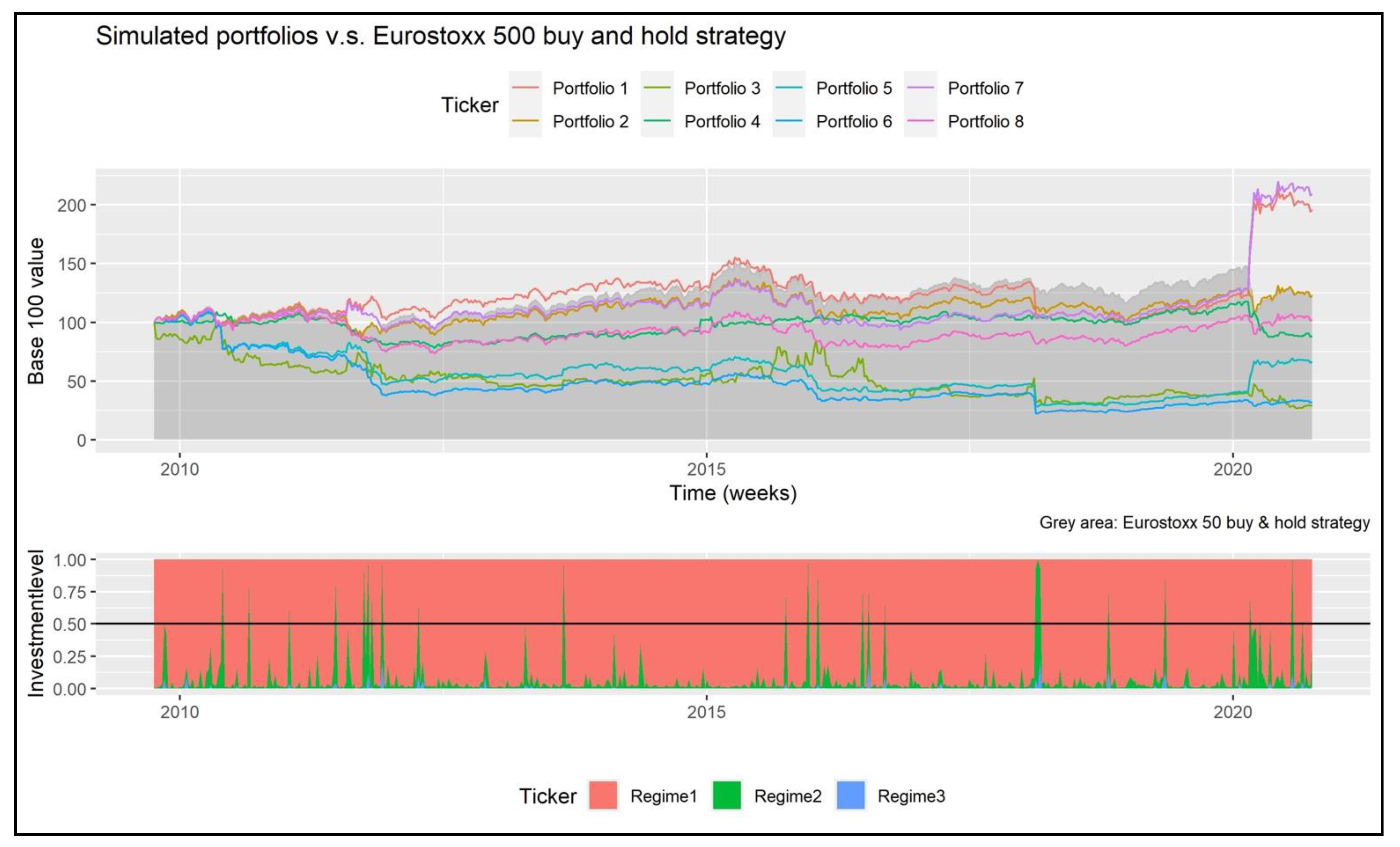
In Figure 2, we show the historical performance of the fully invested (${\omega }_i=100\%\mathrm{if}\xi {}_{s=i,T+1}>50\%$) strategy in the eight simulated portfolios. In that figure, we compare their performance against a theoretical buy-and-hold (BH) ESTOXX50 portfolio (grey area). As noted, only portfolios 1 and 7 showed signs of better performance (19.17% and 35.46% of accumulated return, respectively) than the ESTOXX50 BH portfolio (22.86% according to Table 4). This result occurred only in high and extreme volatility periods (such as the COVID-19 2020-current period).

These results are in line with Alexander, Kapraun, and Korovilas’ [24,25] conclusions given that a stocks/volatility portfolio diversification is useful only in distress periods, as the lower panel (three-regime smoothed probabilities) of Figure 2 shows. Given this, had the investor followed any of these eight simulated trading rules, he/she would not have outperformed a BH ESTOXX50-only portfolio most of the time.

In Figure 3, we present a similar analysis rationale, but in the smoothly invested portfolios (${\omega }_i={\xi }_{s=i,T+1}$). As shown, the portfolio performance improved significantly against the previous weighting method. As noted in the upper panel, portfolios 1, 2, and 7 showed signs of a better performance in several periods (96.02%, 22.83%, and 109.50% of accumulated return, respectively). These are periods in which the VSTOXX and distress levels in the ESTOXX50 market were low (as noted and compared with the lower panel). This result suggests that, for the specific case of an ESTOXX50-VSTOXX-Bundes portfolio, it is preferable to use a smoothed weighting method (as in Brooks and Persand [38]) rather than a security fully invested method.

An interesting result observed in portfolio 1 is the fact that the suggested trading strategy only holds when opposite changes in the ESTOXX50 and the VSTOXX occur (that is, when the negative correlation between these two securities holds). There is a special period in which this relationship did not hold and affected the simulated investor: The 2016–2019 international trade tension started with the new economic and commerce policy of the U.S. In this period, the volatility levels remained relatively low, but the ESTOXX50 still showed some drawback movements due to the trade tension between the European Union or China with the U.S. Given this geopolitical situation, the high ($s=2$) or extreme ($s=3$) regime smoothed probabilities remained low most of the time. This was observed with the jumps in July and September of 2016 and February to March of 2018. These jumps reversed rapidly, given the fast mean-reverting property of volatility.

Given these performance results, a partial conclusion is the fact that the use of MS-GARCH models for stocks-volatility futures trading decisions is useful only in distressed stock market periods. Consistent with this, the use of a smoothed weighting method (${\omega }_i={\xi }_{s=i,T+1}$) led to better performance.

The results of the previous simulations did not include the impact of stock trading fees, but rather only VSTOXX future position’s roll-over costs. By following the suggestions of the previous literature, we present the results of a theoretical investor that paid a 0.1% fee, plus 10% of VAT in the traded amount in the ESTOXX50. The performance results of the security fully invested weighting method are shown in Figure 4 and the results of the smoothed method in Figure 5.

As noted in Figure 4, there is an impact on the performance given the stock-trading fees, but given the small changes made each week in calm ($s=1$) periods, the accumulated return decreased from 19.17% and 35.46%, in portfolios 1 and 7, to 18.39% and 32.54%, respectively.

In a parallel situation to the results of Figure 2, the conclusion of the benefit of the simulated trading strategy holds only in distress periods.

The same result is shown in Figure 5, in which the accumulated return of portfolios 1, 2, and 7 (the best performers in Figure 3 and Figure 5) is higher than the buy-and-hold strategy, but lower than the observed values of Figure 3; that is, these three portfolios paid an accumulated return of 90.91%, 19.61%, and 101.39%, respectively. These returns are lower than the observed returns in Figure 2, given the impact of the trading fees.

To gain a different perspective of the impact of stock trading fees, we simulated the performance of a theoretical institutional investor who paid a 0.08% monthly fee in the monthly mean position in the ESTOXX50. For this purpose, we present the performance of the eight simulated portfolios with a fully invested weighting method in Figure 6 and the smoothed method in Figure 7.

As noted in Figure 6, the impact of stock trading fees eroded the performance of the fully invested weighting method portfolios. For the specific case of this type of weighting method, the accumulated return of portfolio 1 (the best performer in the previous related figures) is marginally lower.

In Figure 7, in which the simulated portfolios used a smoothed weighting method, the performance results hold, as observed in the two previous cases (trading fee-free and individual investor). With this, the accumulated return of portfolios 1, 2, and 7 are 94.99%, 22.18%, and 108.31%, respectively.

A very important result of Figure 2, Figure 3, Figure 4, Figure 5, Figure 6 and Figure 7 is the fact that the simulated algorithm, along with a VSTOXX future diversification strategy, work only in distress periods. During calm ($s=1$) periods or regimes in which the ESTOXX50 market grew or fell with small volatility levels, the diversification benefits and timing did not pay all the time.

Even if the final portfolio performance of three of the smoothly weighted portfolios is high at the end of our simulations, the observed results suggest that this diversification with volatility holds only in the short term. From a longer-term perspective, it is necessary to find diversification alternatives, as the one suggested with Algorithm 3 and tested next.

As mentioned in the Introduction section, we noted in our simulations that portfolio 1 of an institutional investor with a smoothed weighting method (${\omega }_i={\xi }_{s=i,T+1}$) had a higher or at least equal performance to the buy-and-hold ESTOXX50 strategy. Only in the aforementioned February to March of 2018 period, the simulated portfolio fell in value as the ESTOXX50 did, but did not recover until the distress ($s=2$) period of the COVID-19 pandemic took place. This led us to assume that maybe a portfolio with our suggested VSTOXX MS-GARCH trading algorithm is useful in the short term and could be combined with another one with a buy-and-hold ESTOXX50 strategy, that is, to invest in ESTOXX50 stocks in calm periods and to diversify with portfolio 1 in distressed periods.

Given this rationale, we asked: What would happen if a given investor could invest in two ETFs? Specifically, we refer to one ETF that tracks the ESTOXX50 index and another that performs the VSTOXX MS-GARCH trading algorithm, as in portfolio 1 of Figure 7. Based on these questions, we simulated the performance of an individual investor who used a mean-variance portfolio selection process in these two ETFs each week and managed a portfolio that actively allocates money in each.

By using Algorithm 3 to simulate this investor and by using a 0.1% stock trading fee plus 10% VAT in each ETF traded amount, we reached the performance shown in Figure 8 and Figure 9.

In both figures, we present the historical performance of a theoretical investor that paid no stock trading fees (blue line in the upper panel of both figures) and compare it against the performance of a theoretical investor that paid a 0.1% plus 10% VAT trading fee (red line). Additionally, in both figures, the historical performance of the simulated investors is compared against the buy-and-hold ESTOXX50 strategy (grey area in the upper panel of Figure 8) or the historical value of the VSTOXX index (Figure 9). As noted, the impact of ETF (stock) trading fees is marginal in the simulated portfolio performance.

In the lower panels of both figures, we present the historical weight in each ETF, estimated with the optimization problem (20) in Algorithm 3. As noted from the results in both figures, both simulated portfolios invested more in the ESTOXX50 ETF during calm periods in which the stocks grew in value (blue area of lower panel) and more in the simulated VSTOXX diversified ETF (red area) during distress periods.

Specific evidence of this result can be noted in Figure 9 in which the investment level in the ESTOXX50/VSTOXX ETF (portfolio 7) increased when the VSTOXX value increased (evidence of a more distressing period).

Given this result, we summarize that VSTOXX diversification is appropriate in the short term if a given investor uses our suggested MS-GARCH trading algorithm (Algorithm 2). If the goal is to have a long-term benefit, then it is appropriate to combine the suggested trading algorithm in an ETF with an ESTOXX50 buy-and-hold method. This could enhance the performance of a stock portfolio significantly by benefiting from stock growth during calm ($s=1$) periods and the increase in volatility futures’ value in distress ($s=2$) periods.

5. Conclusions and Guidelines for Further Research

Volatility futures represent a very important security since the inception of stock-option-implied volatility indexes. They serve as a gauge of stock market volatility and as diversification security in distressed stock market periods. One limitation of volatility futures is the fact that volatility’s stochastic process is a fast mean-reverting one. Given this, along with the impact of future position roll-over costs, volatility futures have some limitations for a buy-and-hold position and for long-term diversification benefits.

Previous works proved the benefits of volatility portfolio diversification as true in an ex-ante manner. Therefore, there is evidence of mean-variance efficiency or significant benefits in an investor’s volatility function [20,21,22,23,35]. Despite these results, ex-post benefits were proved marginally, given the impact of roll-over costs and stock trading fees [24,25]. These first reviews about volatility future diversification were made in a mean-variance, Black-Litterman [37] optimal portfolio selection rationale. Among their main findings, the authors found that volatility future diversification benefits hold in the short term and only in distressed market periods.

To test another quantitative portfolio selection model for stocks and volatility futures, De la Torre-Torres, Venegas-Martínez, and Martínez-Torre-Enciso [29] tested the use of symmetric Gaussian and t-Student MS-GARCH models. It was performed to forecast the probability of being in distressed ($s=2$) or extremely distressed ($s=3$) periods at $T+1$. By testing their trading algorithm in the S&P 500 stock index and the VIX index volatility, the authors found benefits of volatility futures’ diversification for institutional investors in the short term.

The present paper extended the previous results in two aspects: (1) It tested the benefits of MS-GARCH models for portfolio trading in the Eurostoxx 50 (ESTOXX50) stock index, and the corresponding VSTOXX option implied volatility index’s futures. With the use of weekly historical data, the simulations made suggest that there are performance benefits either for individual or institutional Euro-based portfolios. The results of our simulations include the impact of either roll-over future position costs or the impact of a 0.1% stock trading fee plus 10% of value-added tax (VAT).

We also found that the lack of performance that the simulated portfolios had in some periods has been compensated and turned to overperformance in distress periods such as the one of the COVID-19 pandemic (2020) or the European debt crisis (2013).

Despite this, we found additional ways to enhance an investor’s performance against a buy-and-hold stock (ESTOXX50) only strategy. More specifically, we enhanced our results by simulating the performance that an individual investor would have had, had he/she invested in a portfolio with two securities only:

• An ETF that tracked (with zero tracking-error) the ESTOXX50.
• An ETF that invested in a theoretical portfolio that used our suggested MS-GARCH trading algorithm. An ETF that invested only in ESTOXX50 and VSTOXX.

The results of this second simulation suggest that the simulated performance of this investor is considerably high against an ESTOXX50 buy-and-hold strategy.

Given this, our main findings are that our suggested MS-GARCH trading algorithm is useful for institutional and individual investors in the short term. Additionally, if a given individual or institutional investor invested in the aforementioned two ETF portfolios, his/her performance would increase and could create value with VSTOXX futures or during either distressing periods or do calm periods with stocks.

Our results could be of use for institutional investors. For fund managers (ETF managers), they could offer two securities (fund or ETFs): one that tracks the performance of the ESTOXX50 and another that performs our MS-GARCH ESTOXX50-VSTOXX strategy. During calm market periods, investors would demand their ESTOXX50 fund, and during distressed periods, they could use the ESTOXX50-VSTOXX option. Given this, the ETF or fund manager could benefit from the management fees of both available ETFs and the rebalancing decisions of their customers.

In addition, the strategy could be of use for institutional investors such as pension funds, insurance companies, or endowments by benefiting from the VSTOXX future value during periods of distress and benefiting from stock market growth during calm periods.

Among the guidelines for further research that we suggest, we can mention the use of asymmetric MS-GARCH models and pdfs in the trading algorithm. We also suggest the use of multi-factor or time-varying transition probabilities MS models such as that of Filardo [74,92], or the estimation of MS and MS-GARCH models with neural networks, as in Liao, Yamaka, and Sriboonchita [93]. Weekly historical performance of the eight simula.

As another extension of our work, we suggest extending our review to test the performance of our VSTOXX trading strategy to shorter-term simulation periods, such as daily or even intra-day periods. We suggest this to have a proper record and robustness test of what would be the short-term and long-term benefits (including the impact of roll-over, stock trading fees, and taxes) of our simulated strategies.

Finally, we suggest research of more precise, converging, and computationally efficient algorithms for the estimation of MS-GARCH models. Markov-Chain Monte Carlo methods are very precise and convergent, but they are not computationally efficient.