An Adaptive Proximal Bundle Method with Inexact Oracles for a Class of Nonconvex and Nonsmooth Composite Optimization

Abstract

In this paper, an adaptive proximal bundle method is proposed for a class of nonconvex and nonsmooth composite problems with inexact information. The composite problems are the sum of a finite convex function with inexact information and a nonconvex function. For the nonconvex function, we design the convexification technique and ensure the linearization errors of its augment function to be nonnegative. Then, the sum of the convex function and the augment function is regarded as an approximate function to the primal problem. For the approximate function, we adopt a disaggregate strategy and regard the sum of cutting plane models of the convex function and the augment function as a cutting plane model for the approximate function. Then, we give the adaptive nonconvex proximal bundle method. Meanwhile, for the convex function with inexact information, we utilize the noise management strategy and update the proximal parameter to reduce the influence of inexact information. The method can obtain an approximate solution. Two polynomial functions and six DC problems are referred to in the numerical experiment. The preliminary numerical results show that our algorithm is effective and reliable.

1. Introduction

Consider the following optimization problem:

$$\underset{x\in {\mathbf{R}}^N}{min}\psi \left(x\right):=f\left(x\right)+h\left(x\right),$$

(1)

where $f:{\mathbf{R}}^N\to \mathbf{R}$ is a finite convex function and function h is not necessarily convex. So the primal function (1) may be nonconvex and note that functions f and h are not necessarily smooth. In this paper, we consider the case that function h is easy to evaluate while the function f is much harder to evaluate and is time consuming.

The sum of two functions can be found in many optimization problems such as the Lasso problem in image problems and the optimization problems in machine leaning and so on. Meanwhile, the composite function (1) can be obtained from other problems such as by splitting technique and nonlinear programming and so on. Concretely, in some cases, the function considered is much complicated and difficult to evaluate, to speed up calculations, dividing the primal function into two functions f and h with relatively simple structure is a possible way. Besides that, another way is the penalty strategy which transfers the constraint problem into an unconstrained problem with the sum form.

Note that the splitting type methods (see [1,2]) and the alternating type methods (see [3,4]) are two classes of important methods for composite optimization. When functions f and h have some special structures, the above methods may be effective and own better convergent results. However, if the functions do not own special structures or the functions are much complex and difficult to evaluate, the above methods may not be suitable for Problem (1). Meanwhile, in the alternating direction type methods, at least two subproblems need to be solved at each iteration, if one of the subproblems is difficult or hard to solve, the algorithms’ effectiveness may be slowed down. Then, it is meaningful to seek other suitable methods to deal with Problem (1) without special structures.

In recent years, many scholars have devoted time to seeking effective methods for nonconvex and nonsmooth optimization problems, see [5,6,7,8,9,10,11,12,13,14,15,16,17,18,19,20]. Usually, bundle methods are much effective for solving nonsmooth optimization problems [21,22,23,24,25,26]. Bundle methods use “black box” to compute the objective value and one of its subgradients (not special) at each iterations. Then, bundle techniques can be a class of possible effective ways to deal with the composite problem (1). At present, the proximal alternating linearization type methods (see [4,27,28,29]) are one effective kind of bundle methods for some composite problems. They need to solve two subproblems at each iteration and the data referred are usually exact. When inexact oracles are involved, the above methods may not be suitable and even be not convergent.

In this paper, we design a proximal bundle method for the inexact composite problem (1) and update the proximal parameter $\mu$ to reduce the effects of the inexact information. In the following, we first present some cases where inexact evaluations are generated.

Inexact evaluations are usually referred to in stochastic programming and Lagrangian relaxation [30,31]. It is at the very least impractical and is usually not even easy to solve those subproblems exactly. In bundle methods, inexact information are obtained from inexact oracles. There are different types of inexact oracles. In our work, we consider the Upper oracle (see (2a)–(2c) below). The Upper oracles may overestimate the corresponding function values and get negative linearization errors even if the primal function is convex.

In this paper, we focus on a class of nonconvex and nonsmooth composite problems with inexact data. The design and convergence analysis of bundle methods for nonconvex problems with inexact function and subgradient evaluations are quite involved and there are only a handful of papers for this topic, see [15,32,33,34,35].

In this paper, we present a proximal bundle method with a convexification technique and noise management strategy to solve composite problem (1). Concretely, we design “convexification” technique for the nonconvex function h to make sure the corresponding linearization error nonnegative and then we adopt the noise management strategy for inexact function f. If the error is “too ” large and the testing condition (22) is not satisfied, we decrease the value of the proximal parameter $\mu$ to obtain better iterative point. We summary our work as follows:

• Firstly, we design the convexification technique for the nonconvex function h to make sure the linearization errors of the augment function ${\varphi }_n=h+\frac{{\eta }_n}{2}{\parallel ·\parallel }^2$ are nonnegative. Note that the the augment function ${\varphi }_n$ may not be a convex function, the nonnegative linearization errors can be obtained by the choices of the parameter ${\eta }_n$. Similar strategy can also be seen in [10,11,15,16].
• Then, the sum of functions f and ${\varphi }_n$ is regarded as an approximate function for the composite function (1). We construct respectively the cutting plane models for functions f and ${\varphi }_n$ and regard the sum of the two cutting plane models as the cutting plane model for the approximate function which may be a better cutting plane model. It should be noted that since inexact information are referred, the corresponding cutting plane model may not always be below function f.
• Although we design the cutting plane models for functions f and ${\phi }_n$, respectively, only one quadratic programming (QP) subproblem needs to be solved at each iteration. By the construction of cutting plane models, we have that the QP subproblem is strictly convex and has unique solution which makes our algorithm more effective.
• In the method, we construct the noise management step to deal with the inexact data for function values and subgradient values where the errors are only bounded and need not to vanish. If the noise error is “too” large and the testing condition (22) is not satisfied, we decrease the value of $\mu$ to obtain a better iterative point.
• Two polynomial functions with twenty different dimensions and six DC (difference of convex) problems are referred to in the numerical experiment. In exact cases, our method is comparable with the method in [16] and has higher precision. In five different types of inexact oracles, we obtain that the exact case has the best performance and the performance of the vanishing error cases are generally better than that in the constant error cases. We also apply our method to six DC problems and the results show that our algorithm is effective and reliable.

The remainder of this paper is organized as follows. In Section 2, we review some variational analysis definitions and some preliminaries for proximal bundle method. Our proximal bundle method is given in Section 3. In Section 4, we present the convergent property of the algorithm. Some preliminary numerical testings are implemented in Section 5. In Section 6, we give some conclusions.

2. Preliminaries

In this section, we firstly review some concepts and definitions and then present some preliminaries for a proximal bundle method.

2.1. Preliminary

In this subsection, we recall concepts and results of variational analysis that will be used in the latter of the paper. The definition of lower-${\mathcal{C}}^k$ is given in Definition 10.29 in [36]. For completeness, we state it as follows:

Definition 1.

A function $F:\mathcal{O}\to \mathbf{R}$, where $\mathcal{O}$ is an open subset of ${\mathbf{R}}^N$, is said to be lower-${\mathcal{C}}^k$ on $\mathcal{O}$, if on some neighborhood V of each $\widehat{x}\in \mathcal{O}$, there is a representation:

$$F\left(x\right)=\underset{t\in T}{max}{F}_t\left(x\right),$$

in which the function $F_t$ are of class $C^k$ on V and the index set T is a compact space such that $F_t\left(x\right)$ and all its partial derivatives through order k depend continuously not just on x but on $(t,x)\in T\times V$.

If $k=2$, F is a lower-${\mathcal{C}}^2$ function. lower-${\mathcal{C}}^2$ function has a special relationship with convexity, see Theorem 10.33 in [36]. We state its equivalent statement as follow: A function F is lower-${\mathcal{C}}^2$ on an open set $\mathcal{O}\subseteq {\mathbf{R}}^N$ if F is finite on $\mathcal{O}$ and for any $x\in \mathcal{O}$, there exists a threshold $\overline{\lambda }\ge 0$ such that $F+\frac{\lambda }{2}{\parallel ·\parallel }^2$ is convex on an open neighborhood V of x for all $\lambda \ge \overline{\lambda }$. Specifically, if the function F is convex and finite-valued, then F is lower-${\mathcal{C}}^2$ with threshold $\overline{\lambda }=0$.

For nonconvex function h, in the following, we consider that h is a lower-${\mathcal{C}}^2$ function. Since functions f and h are all not necessarily smooth, then the composite function (1) is also not necessarily smooth. For proper convex function f, the common subdifferential in convex analysis is used, which is denoted by $\partial f\left(x\right)$ at the point $x\in {\mathbf{R}}^N$ (see in [37]). For proper and regular function h, we utilize the limiting subdifferential and also denote it by $\partial h\left(x\right)$ at point x (see in [36]). The definition of the limiting subdifferential is as follows:

$$\partial h\left(x\right):=\underset{y\to x,h\left(y\right)\to h\left(x\right)}{lim\; sup}\left\{v|\underset{u\to y,u\ne y}{lim\; inf}\frac{h\left(u\right)-h\left(y\right)-⟨v,u-y⟩}{\parallel u-y\parallel }\ge 0\right\}.$$

In nonsmooth analysis for convex function f, $\epsilon -\mathrm{subdifferential}$ at point $x^k$ is usually used, which is defined:

$${\partial }_{\epsilon }f\left(x^k\right):=\left\{g|f\left(x\right)\ge f\left(x^k\right)-\epsilon +⟨g,x-x^k⟩\right\},$$

where $\epsilon \ge 0$. In the following, we present the inexact data for function f and give some preliminaries for proximal bundle method.

2.2. Inexact Information and Bundle Construction

Bundle methods are much effective for nonsmooth problems and always utilize “black box” to compute function value and one subgradient at each iterative point. It should be noted that the obtained subgradient is not special. Along the iterative progress, the generated points are divided into two styles: null points, used essentially to increase the model’s accuracy; serious points, significantly decreasing the objective function (and also improve the approximate model’s accuracy). The corresponding iterations are respectively called null steps and serious steps. In the literature, serious points are sometimes called as prox-center or stability center, denoted by ${\widehat{x}}^{k\left(n\right)}$. Then, the sequence $\left\{{\widehat{x}}^{k\left(n\right)}\right\}$ is a subsequence of the sequence $\left\{x^n\right\}$. For notation simplification, we write ${\widehat{x}}^k={\widehat{x}}^{k\left(n\right)}$.

For function f, the oracle can only provide inexact function value and one subgradient value at each iteration, ${\widehat{f}}^l:=f_{x^l},{\widehat{g}}_f^l:=g_f^{x^l}$, with unknown but bounded inaccuracy. That is, for $\forall x^l\in {\mathbf{R}}^N$, we have

$${\widehat{f}}^l\ge f\left(x^l\right)-{\theta }_l,$$

(2a)

$$f(·)\ge {\widehat{f}}^l+⟨{\widehat{g}}_f^l,·-x^l⟩-{\epsilon }_l,$$

(2b)

Meanwhile

$${\theta }_l\le \overline{\theta },\mathrm{and}{\epsilon }_l\le \overline{\epsilon }.$$

(2c)

According to (2a)–(2c), we have the following relationships

$$\begin{array}{c}\hfill \left\{\begin{array}{c}{\widehat{g}}_f^l\in {\partial }_{{\theta }_l+{\epsilon }_l}f\left(x^l\right),\hfill \\ {\widehat{f}}^l\in [f\left(x^l\right)-{\theta }_l,f\left(x^l\right)+{\epsilon }_l].\hfill \end{array}\right.\end{array}$$

(3)

Note that we only require the relationship ${\theta }_l+{\epsilon }_l\ge 0$ holds for each index l. The bundle for function f can be noted as

$${\mathrm{B}}_k^f:=\left\{\left(x^l,{\widehat{f}}^l=f_{x^l},{\widehat{g}}_f^l\in \partial f_{x^l}\right),l\in I_n\right\},$$

(4)

Now we present the cutting plane model of function f by the inexact information:

$${\tilde{\phi }}_n\left(x\right)=\underset{l\in I_n}{max}\left\{{\widehat{f}}^l+⟨{\widehat{g}}_f^l,x-x^l⟩\right\}={\widehat{f}}^{\overline{k}}+\underset{l\in I_n}{max}\left\{-e_{f,l}^k+⟨{\widehat{g}}_f^l,x-{\widehat{x}}^k⟩\right\},$$

(5)

where ${\widehat{f}}^{\overline{k}}=f_{x^{k\left(n\right)}}$, ${\widehat{x}}^k=x^{k\left(n\right)}$ is the current stability center with index $k\left(n\right)$ corresponding to its candidate point index and $e_{f,l}^k$ is linearization errors, which measures the difference between cutting planes and the function value computed in the oracle for the current serious point, that is

$$e_{f,l}^k={\widehat{f}}^{\overline{k}}-{\widehat{f}}^l-⟨{\widehat{g}}_f^l,{\widehat{x}}^k-x^l⟩.$$

(6)

Especially, note that the relation ${\tilde{\phi }}_n\left(x\right)\le f\left(x\right)$ does not necessarily hold. So the linearization error $e_{f,l}^k$ may be negative. In fact, by (2a), (2b) and (6), $e_{f,l}^k$ satisfies that

$$e_{f,l}^k\ge -({\theta }_{k\left(n\right)}+{\epsilon }_l).$$

(7)

Meanwhile, cutting plane model ${\tilde{\phi }}_n$ may overestimate f at some points. By (2b), the following inequality holds

$${\tilde{\phi }}_n\left(x\right)\le f\left(x\right)+\underset{l\in I_n}{max}{\epsilon }_l.$$

(8)

For nonconvex function h, linearization errors may be nonnegative. In bundle methods, nonnegative linearization errors are much important for the convergence. For that we present a local “convexification” technique, similar techniques can also be seen in [15,16,38]. For the convexification parameter ${\eta }_n$, its choice is as follows

$${\eta }_n\ge {\eta }_n^{min}=max\left\{-\frac{e_{h,l}^k}{\frac{1}{2}{\parallel x^l-{\widehat{x}}^k\parallel }^2}\right\},\mathrm{with}l\in I_n,\mathrm{and}\parallel x^l-{\widehat{x}}^k{\parallel }^2\ne 0,$$

(9)

where $I_n$ denotes an index set, i.e., $I_n\subseteq \{0,1,2,\cdots \}$ and $e_{h,l}^k$ is the linearization error of h, which is defined as follows with $h^l=h\left(x^l\right),g_h^l\in \partial h\left(x^l\right)$

$$e_{h,l}^k:=h\left({\widehat{x}}^k\right)-h^l-⟨g_h^l,{\widehat{x}}^k-x^l⟩.$$

The bundle for function h can be noted as

$${\mathrm{B}}_k^h:=\left\{\left(x^l,h^l=h\left(x^l\right),g_h^l\in \partial h\left(x^l\right)\right),l\in I_n\right\},$$

(10)

Next, we introduce the augment function ${\varphi }_n$ of f, it is defined by

$${\varphi }_n\left(x\right):=h\left(x\right)+\frac{{\eta }_n}{2}{\parallel x-{\widehat{x}}^k\parallel }^2,\forall x\in {\mathbf{R}}^N,$$

(11)

where ${\eta }_n\ge {\eta }_n^{min}$ holds. Note that by the definition of ${\varphi }_n$, we have $h\left({\widehat{x}}^k\right)={\varphi }_n\left({\widehat{x}}^k\right)$. By the calculation of subgradient, we have there exists $g_h^l\in \partial h\left(x^l\right)$ satisfying

$$g_{\varphi }^l=g_h^l+{\eta }_n(x^l-{\widehat{x}}^k)\in \partial {\varphi }_n\left(x^l\right).$$

Meanwhile, the linearization error of function ${\varphi }_n$ is

$$\begin{array}{cc}{e}_{\varphi ,l}^k\hfill & {\displaystyle ={\varphi }_n\left({\widehat{x}}^k\right)-{\varphi }_n\left(x^l\right)-⟨g_{\varphi }^l,{\widehat{x}}^k-x^l⟩}\hfill \\ \hfill & {\displaystyle =h\left({\widehat{x}}^k\right)-h\left(x^l\right)-\frac{{\eta }_n}{2}\parallel x^l-{\widehat{x}}^k{\parallel }^2-⟨g_h^l+{\eta }_n(x^l-{\widehat{x}}^k),{\widehat{x}}^k-x^l⟩=e_{h,l}^k+\frac{{\eta }_n}{2}{\parallel x^l-{\widehat{x}}^k\parallel }^2.}\hfill \end{array}$$

(12)

By the choice of the convexification parameter ${\eta }_n$, we have $e_{\varphi ,l}^k\ge 0$ holds for all $l\in I_n$.

In the following, we regard the sum of functions f and ${\varphi }_n$ as an approximate function for composite function (1):

$${\Psi }_n\left(x\right)=f\left(x\right)+{\varphi }_n\left(x\right).$$

(13)

For (13), we utilize the sum of cutting plane models of functions f and ${\varphi }_n$ as the cutting plane model. The cutting plane model of the augment function ${\varphi }_n$ is defined as follows

$${\tilde{\varphi }}_n\left(x\right)=\underset{l\in I_n}{max}\left\{{\varphi }_n\left(x^l\right)+⟨g_{\varphi }^l,x-x^l⟩\right\}.$$

Its equivalent form is

$$\begin{array}{cc}\hfill {\tilde{\varphi }}_n\left(x\right)=& {\varphi }_n\left({\widehat{x}}^k\right)+\underset{l\in I_n}{max}\left\{-e_{\varphi ,l}^k+⟨g_{\varphi }^l,x-{\widehat{x}}^k⟩\right\}\hfill \\ \hfill =& h\left({\widehat{x}}^k\right)+\underset{l\in I_n}{max}\left\{-\left(e_{h,l}^k+\frac{{\eta }_n}{2}{\parallel x^l-{\widehat{x}}^k\parallel }^2\right)+⟨g_h^l+{\eta }_n(x^l-{\widehat{x}}^k),x-{\widehat{x}}^k⟩\right\}.\hfill \end{array}$$

(14)

Then, the cutting plane model for the approximate function ${\Psi }_n$ is

$${\Phi }_n\left(x\right)={\tilde{\phi }}_n\left(x\right)+{\tilde{\varphi }}_n\left(x\right).$$

The new iterative point $x^{n+1}$ is given by the following QP (quadratic programming) subproblem

$$x^{n+1}:=arg\underset{x\in {\mathbf{R}}^N}{min}\left\{{\tilde{\phi }}_n\left(x\right)+{\tilde{\varphi }}_n\left(x\right)+\frac{{\mu }_n}{2}{\parallel x-{\widehat{x}}^k\parallel }^2\right\}=arg\underset{x\in {\mathbf{R}}^N}{min}\left\{{\Phi }_n\left(x\right)+\frac{{\mu }_n}{2}{\parallel x-{\widehat{x}}^k\parallel }^2\right\},$$

(15)

where ${\mu }_n>0$ is the proximal parameter. Note that $x^{n+1}$ is the unique solution to (15) by strong convexity. The following lemma shows the relation between the current stationary center and the new generated point. Similar conclusion can also be seen in Lemma 10.8 in [39] which is for convex function. Here we omit the proof.

Lemma 1.

Let $x^{n+1}$ be the unique solution to the QP subproblem (15) and proximal parameter ${\mu }_n>0$. Then, we have

$$x^{n+1}={\widehat{x}}^k-\frac{1}{{\mu }_n}{G}^n,$$

(16a)

where

$$G^n:=\sum _{l\in I_n}{\alpha }_1^l{\widehat{g}}_f^l+\sum _{l\in I_n}{\alpha }_2^l\left(g_h^l+{\eta }_n(x^l-{\widehat{x}}^k)\right).$$

(16b)

Meanwhile ${\alpha }_1=({\alpha }_1^1,\cdots ,{\alpha }_1^n)$ and ${\alpha }_2=({\alpha }_2^1,\cdots ,{\alpha }_2^n)$ is the solution to

$$\left\{\begin{array}{cc}{\displaystyle \underset{{\alpha }_1,{\alpha }_2\in {\mathbf{R}}_{+}^{|I_n|}}{min}}\hfill & \frac{1}{2{\mu }_n}{∥G^n∥}^2+\sum _{l\in I_n}{\alpha }_1^l{e}_{f,l}^k+\sum _{l\in I_n}{\alpha }_2^l{e}_{\varphi ,l}^k\hfill \\ {\displaystyle s.t.}\hfill & {\alpha }_1,{\alpha }_2\in S_n:=\left\{z\in {[0,1]}^{|I_n|}:\sum _{l\in I_n}{z}^l=1\right\}.\hfill \end{array}\right.$$

(17)

In addition, the following relations hold:

(i) 

${\displaystyle G^n\in \partial {\Phi }_n\left(x^{n+1}\right)}$;

(ii) 

${\displaystyle {\widehat{f}}^{\overline{k}}+{\varphi }_n\left({\widehat{x}}^k\right)-{\Phi }_n\left(x^{n+1}\right)={\mu }_n{\parallel x^{n+1}-{\widehat{x}}^k\parallel }^2+\sum _{l\in I_n}{\alpha }_1^l{e}_{f,l}^k+\sum _{l\in I_n}{\alpha }_2^l{e}_{\varphi ,l}^k}$.

In the following, we present the concepts of the predict descent. Concretely, the predict descent for functions $f,{\varphi }_n,{\Psi }_n$ are stated as follows

$$\begin{array}{c}\hfill \left\{\begin{array}{c}{\displaystyle {\delta }_{n+1}^f={\widehat{f}}^{\overline{k}}-{\tilde{\phi }}_n\left(x^{n+1}\right),}\hfill \\ {\displaystyle {\delta }_{n+1}^{\varphi }=h\left({\widehat{x}}^k\right)+\frac{{\eta }_n}{2}{\parallel x^{n+1}-{\widehat{x}}^k\parallel }^2-{\tilde{\varphi }}_n\left(x^{n+1}\right),}\hfill \\ {\displaystyle {\delta }_{n+1}={\delta }_{n+1}^f+{\delta }_{n+1}^{\varphi }.}\hfill \end{array}\right.\end{array}$$

(18)

Note that the predict descent is much important for the convergence of bundle methods. By the definitions of functions ${\varphi }_n$ and ${\tilde{\varphi }}_n$, we have ${\delta }_{n+1}^{\varphi }\ge 0$. Since inexact data are referred to in the computation of function f, the nonnegativity of ${\delta }_{n+1}^f$ can not be guaranteed. Hence the nonnegativity of ${\delta }_{n+1}$ can not be guaranteed too.

Next we give the aggregate linearization error which is defined by

$$e_{n+1}:=\sum _{i\in I_n}{\alpha }_1^l{e}_{f,l}^k+\sum _{l\in I_n}{\alpha }_2^l{e}_{\varphi ,l}^k.$$

(19)

By the term (ii) in Lemma 1 and the definition of ${\delta }_{n+1}$ in (18), the following relationship holds

$$\begin{array}{cc}{\delta }_{n+1}\hfill & {\displaystyle =\frac{\parallel G^n{\parallel }^2}{{\mu }_n}+\frac{{\eta }_n}{2}{\parallel x^{n+1}-{\widehat{x}}^k\parallel }^2+e_{n+1}}\hfill \\ \hfill & {\displaystyle =\frac{R_n+{\mu }_n}{2}{\parallel x^{n+1}-{\widehat{x}}^k\parallel }^2+e_{n+1},}\hfill \end{array}$$

(20)

where $R_n={\mu }_n+{\eta }_n$. Next we define the aggregate linearization for approximate model ${\Phi }_n$:

$${\Phi }_n^{lin}\left(x\right):={\Phi }_n\left(x^{n+1}\right)+⟨G^n,x-x^{n+1}⟩.$$

Then, the aggregate linearization error can be also expressed as the difference between the value of the oracle at the current serious point and the value of aggregate linearization ${\Phi }_n^{lin}$ at that point, that is,

$$e_{n+1}={\widehat{f}}^{\overline{k}}+h\left({\widehat{x}}^k\right)-{\Phi }_n^{lin}\left({\widehat{x}}^k\right).$$

Indeed, by the definition of ${\Phi }_n^{lin}\left(x\right)$, we have

$${\Phi }_n^{lin}\left(x\right)={\widehat{f}}^{\overline{k}}+h\left({\widehat{x}}^k\right)+⟨G^n,x-{\widehat{x}}^k⟩-e_{n+1}.$$

By the convexity of function ${\Phi }_n$, the inequality ${\Phi }_n\left(x\right)\ge {\Phi }_n^{lin}\left(x\right)$ holds. So for any $x\in {\mathbf{R}}^N$, we have

$${\widehat{f}}^{\overline{k}}+h\left({\widehat{x}}^k\right)\le {\Phi }_n\left(x\right)-⟨G^n,x-{\widehat{x}}^k⟩+e_{n+1}.$$

By (8), the following inequality holds under the condition ${\tilde{\varphi }}_n\left(x\right)\le {\varphi }_n\left(x\right)$:

$${\widehat{f}}^{\overline{k}}+h\left({\widehat{x}}^k\right)\le \psi \left(x\right)+\frac{{\eta }_n}{2}{\parallel x-{\widehat{x}}^k\parallel }^2+\underset{l\in I_n}{max}{\epsilon }_l-⟨G^n,x-{\widehat{x}}^k⟩+e_{n+1}.$$

(21)

Note that the condition ${\tilde{\varphi }}_n\left(x\right)\le {\varphi }_n\left(x\right)$ may not be hold if the convexification parameter ${\eta }_n$ is less that the threshold parameter $\overline{\rho }$ (the function ${\varphi }_n\left(x\right)$ may not be convex), but the choice of ${\eta }_n$ ensures the nonnegativity of $e_{\varphi ,l}^k$ for all $l\in I_n$.

By the nonnegativity of $e_{\varphi ,l}^k$ and (7), the aggregate linearization error satisfies

$$e_{n+1}\ge -\left({\theta }_{k\left(n\right)}+\sum _{l\in I_n}{\alpha }_1^l{\epsilon }_l\right)\ge -\left(\overline{\theta }+\overline{\epsilon }\right).$$

Using the fact that $x^{n+1}$ is the solution of the QP problem (15) and the definition of predict descent in (18), we have that

$$\begin{array}{ccc}\hfill {\delta }_{n+1}& \ge & \frac{{\mu }_n}{2}{\parallel x^{n+1}-{\widehat{x}}^k\parallel }^2-\left({\tilde{\phi }}_n\left({\widehat{x}}^k\right)+{\tilde{\varphi }}_n\left({\widehat{x}}^k\right)-{\widehat{f}}^{\overline{k}}-{\varphi }_n\left({\widehat{x}}^k\right)-\frac{{\eta }_n}{2}{\parallel x^{n+1}-{\widehat{x}}^k\parallel }^2\right)\hfill \\ & \ge & \frac{{\mu }_n}{2}\parallel x^{n+1}-{\widehat{x}}^k{\parallel }^2+\frac{{\eta }_n}{2}{\parallel x^{n+1}-{\widehat{x}}^k\parallel }^2-\left({\tilde{\phi }}_n\left({\widehat{x}}^k\right)-{\widehat{f}}^{\overline{k}}\right)\hfill \\ & =& \frac{R_n}{2}{\parallel x^{n+1}-{\widehat{x}}^k\parallel }^2-\left({\tilde{\phi }}_n\left({\widehat{x}}^k\right)-{\widehat{f}}^{\overline{k}}\right),\hfill \end{array}$$

where the second inequality follows from the nonnegativity of $e_{\varphi ,l}^k$. By (5) and $x={\widehat{x}}^k$, we have ${\tilde{\phi }}_n\left({\widehat{x}}^k\right)-{\widehat{f}}^{\overline{k}}={max}_{l\in {\mathrm{B}}_n^f}\left\{-e_{f,l}^k\right\}$ holds, Note that if only “small” errors have been introduced into the model ${\Phi }_n$, then it holds

$${\delta }_{n+1}>\frac{{\eta }_n}{2}\parallel x^{n+1}-{\widehat{x}}^k{\parallel }^2+\frac{{\mu }_n}{2}\parallel x^{n+1}-{\widehat{x}}^k{\parallel }^2=\frac{R_n}{2}{\parallel x^{n+1}-{\widehat{x}}^k\parallel }^2.$$

(22)

Then, by (20) and (16), (22) has the following equivalent forms:

$$\begin{array}{c}\hfill \left\{\begin{array}{c}\left(22\right)\mathrm{holds},\mathrm{if}\mathrm{and}\mathrm{only}\mathrm{if}\frac{\parallel G^n{\parallel }^2}{2{\mu }_n}>-e_{n+1},\hfill \\ \left(22\right)\mathrm{holds},\mathrm{if}\mathrm{and}\mathrm{only}\mathrm{if}{\delta }_{n+1}>\frac{\parallel G^n{\parallel }^2}{2{\mu }_n}+\frac{{\eta }_n}{2}{\parallel x^{n+1}-{\widehat{x}}^k\parallel }^2.\hfill \end{array}\right.\end{array}$$

(23)

Next, we present a optimality measure. Concretely, it is that

$${\mathrm{V}}_n:=max\{\parallel G^n\parallel ,e_{n+1}\}.$$

By the above discussions, we have

$$\begin{array}{c}\hfill \left\{\begin{array}{c}{\mathrm{V}}_n\le max\left\{\sqrt{2{\mu }_n{\delta }_{n+1}},{\delta }_{n+1}\right\},\mathrm{if}\left(22\right)\mathrm{holds},\hfill \\ {\mathrm{V}}_n\le \sqrt{-2{\mu }_n{e}_{n+1}}\le \sqrt{2{\mu }_n(\overline{\theta }+\overline{\epsilon }}),\mathrm{otherwise}.\hfill \end{array}\right.\end{array}$$

(24)

From the above inequalities, the smaller ${\mu }_n$ may lead to higher probability to make inequality (22) hold. Based on that, we will update the parameter ${\mu }_n$ to reduce the effects of errors. In the next section, we will give our proximal bundle algorithm for the primal composite problem (1) with inexact information.

3. Algorithm

In this section, we present our adaptive bundle algorithm to composite problem (1) with inexact information. To handle inexact information, similar to [17], we introduce the noise management step. Concretely, when the condition (22) does not hold, ${\mu }_n$ is reduced in order to make ${\delta }_{n+2}>{\delta }_{n+1}$ and increase the probability of condition (22).

Algorithm 1 (Nonconvex Nonsmooth Adaptive Proximal Bundle Method with Inexact Information for a class of composite optimization)

Step 0 (Input and Initialization):          Choose initial point $x^0\in {\mathbf{R}}^N$, constants $\kappa ,m_1\in \left(0,1\right)$, an unacceptable increase parameter $M_0>0$, ${\mu }_{max}>0,R_0>0,\tau >1,\gamma \ge 1$ and a stopping tolerance $Tol\ge 0$. Set noise management parameter NMP = 0 and ${\widehat{x}}^0=x^0$. Set $({\eta }_0,{\mu }_0)=(0,R_0)$. Call the black box to compute $f_{{\widehat{x}}^0},g_{{\widehat{x}}^0}^0,h\left({\widehat{x}}^0\right),g_{h,0}^0$. Set $n=k=0$.

Step 1 (Model generation and QP subproblem):          Having the current proximal center ${\widehat{x}}^k$, the current bundles ${\mathrm{B}}_n^f$ and ${\mathrm{B}}_n^h$ with index set $I_n$, and the current proximal parameter ${\mu }_n$ and the convexification parameter ${\eta }_n$. Having the current approximate models ${\tilde{\phi }}_n\left(x\right)$ and ${\tilde{\varphi }}_n\left(x\right)$. Compute the QP problem (15) to get the next iterative point $x^{n+1}$ and simplex multipliers $({\alpha }_1,{\alpha }_2)$. Then, compute $G^n,{\delta }_{n+1},e_{n+1}$ and $V_n$.

Step 2 (Stopping criterion):          If ${\mathrm{V}}_n\le Tol$, then stop. Otherwise, go to Step 3.

Step 3 (Noise Management):          If relationship (22) does not hold, set $NMP=1$, ${\mu }_{n+1}=\kappa {\mu }_n$, $n:=n+1$, go to Step 1; otherwise, set $NMP=0$ and we call the noise is acceptable and go to Step 4.

Step 4 (Descent testing):         Call the black box to compute $({\widehat{f}}^{n+1},{\widehat{g}}_f^{n+1})$ and $(h^{n+1},g_h^{n+1})$. Check the descent condition $${\widehat{f}}^{\overline{k}}+h\left({\widehat{x}}^k\right)-{\widehat{f}}^{n+1}-h^{n+1}-\frac{{\eta }_n}{2}{\parallel x^{n+1}-{\widehat{x}}^k\parallel }^2\ge m_1{\delta }_{n+1},$$ (25) if (25) does not hold, then declare a null step, and set $k(n+1)=k\left(n\right)$. If $\mathrm{NMP}=0$, choose ${\mu }_{n+1}\in [\gamma {\mu }_n,{\mu }_{max}]$; else if NMP = 1, take ${\mu }_{n+1}={\mu }_n$. Update the bundle information and go to Step 5. Otherwise, declare a serious step. Set ${\widehat{x}}^{k+1}=x^{n+1}, \mathrm{NMP}=0,f_{{\widehat{x}}^{k+1}}=f_{x^{n+1}},k(n+1)=k+1$ and choose ${\mu }_{n+1}={\mu }_n$, update the bundle information and go to Step 5.

Step 5 (Update parameter):         Apply the rule to compute ${\eta }_{n+1}$ $$\begin{array}{c}\hfill \left\{\begin{array}{cc}\hfill & {\eta }_{n+1}={\eta }_n,\mathrm{if}{\eta }_n\ge {\eta }_{n+1}^{min},\hfill \\ \hfill & {\eta }_{n+1}=\tau {\eta }_{n+1}^{min},\mathrm{if}{\eta }_n<{\eta }_{n+1}^{min},\hfill \end{array}\right.\end{array}$$ (26) where ${\eta }_n^{min}$ is given by (9), written with n replaced by $n+1$.

Step 6 (Restart step):           If $\psi \left(x^{n+1}\right)>\psi \left({\widehat{x}}^k\right)+M_0$ holds, then the objective increase is unacceptable; Restart the algorithm by setting $${\eta }_0:={\eta }_n,{\mu }_0:=\tau {\mu }_n,R_0:={\eta }_0+{\mu }_0,$$ $$x^0:={\widehat{x}}^k,k\left(0\right):=0,i_0:=0,I_0:=\left\{0\right\},n:=0,$$ where $i_k$ is the index of serious points. Then, loop to Step 1; otherwise, increase k by 1 in the case of the serious step. In all cases, increase n by 1, and loop to Step 1.

Remark 1.

Note that in Algorithm 1, the update of elements in bundles are not stated clearly. For null step and serious step, the updating strategies are different. When a serious step occurs, the new generated point is regarded as a new proximal center and the corresponding linearization errors in the bundles all should be updated. When a null step emerges, the proximal center keeps unchanged and only the new generated information are added into the bundles to improve the model’s accuracy. As the iterations proceed, the elements in the bundles may be too large that reduces the efficiency of the algorithm. Then, the active technology (only the active element ${\alpha }_1^l$ and ${\alpha }_2^l$ are kept in the bundles) and the compression strategy can be adopted. For the compression strategy, the number of elements in the bundles can be at least two, the aggregate information and the new generated information. It should be noted that although the compression strategy does not impair the convergence of the algorithm, it may affect the model’s effectiveness if the number of elements in the bundles is too small.

In the following, we will focus on the analysis of Algorithm 1 which indicates the algorithm is well defined. If the algorithm loops forever, three situations may occur (the number of restart steps are finite, which can be see in Lemma 3 ):

• an very large loop of noise management between Step 1 and Step 3, driving ${\mu }_n\to 0$;
• a finite number of serious steps, followed by an very large number of null steps;
• an very large number of serious steps.

Next, we firstly give the case of very large loop of noise management.

Lemma 2.

If an very large loop between Step 1 and Step 3 in Algorithm 1 occurs, then the optimal measure ${\mathrm{V}}_n\to 0$.

Proof. 

Suppose an very large loop between Step 1 and Step 3 begins at iterative index $\overline{l}$. According to the algorithm, this means that for all $n\ge \overline{l}$, neither the proximal center ${\widehat{x}}^{k\left(n\right)}={\widehat{x}}^{k\left(\overline{l}\right)}$ nor the approximate models ${\tilde{\phi }}_n,{\tilde{\varphi }}_n,{\Phi }_n$ change. Hence, when solving sequentially the QP optimization problem (15), only parameter ${\mu }_n$ is updated. By the strategy for ${\mu }_n$, we have ${\mu }_n={\kappa }^{n-\overline{l}}{\mu }_{\overline{l}}$, then it holds ${\mu }_n\to 0$ as $n\to \infty$ by $\kappa \in (0,1)$. Using (24), we have

$$0\le {\mathrm{V}}_n\le \sqrt{2{\mu }_n(\overline{\theta }+\overline{\epsilon }})\to 0,{\mu }_n\to 0\mathrm{when}n\to \infty .$$

Then, the proof is completed. □

Note that if very large noise management steps happen, there is finite number of update for the convexification parameter ${\eta }_n$. Then, ${\eta }_n$ eventually is bounded. Before the last two cases, we show that there is only finite number of restart steps in Algorithm 1. For that, we make an assumption, which can also be founded in [16].

Assumption 1.

The following level set $\mathcal{T}:=\{x\in {\mathbf{R}}^N:\psi \left(x\right)\le \psi \left({\widehat{x}}^0\right)+M_0\}$ is nonempty and compact.

By the definition of lower-${\mathcal{C}}^2$, the compactness of set $\mathcal{T}$ and the finite covering theorem, there exists a threshold $\overline{\rho }$ such that for all $\eta \ge \overline{\rho }$, the augmented function $h\left(x\right)+\eta \parallel x-{\widehat{x}}^k{\parallel }^2/2$ is convex for $\forall x,{\widehat{x}}^k\in \mathcal{T}$.

The compactness of $\mathcal{T}$ allows us to find Lipschitz constants for functions f and h, named $L_f$ and $L_h$ respectively (by lower-${\mathcal{C}}^2$ function’s local lipschitz property and the finite covering theorem). The following lemma indicates that the restart step in Algorithm 1 is finite.

Lemma 3.

Suppose only finite number of the noise management steps occur, Assumption 1 holds and consider the sequence of iterative points $\left\{x^n\right\}$ generated by Algorithm 1. The index $l_k\in I_n$ denotes the current proximal center index, then there can be only a finite number of restart steps in Algorithm 1. Hence, eventually the sequence $\{{\widehat{x}}^k\}$ is entirely in $\mathcal{T}$.

Proof. 

Firstly, new iterative point $x^{n+1}$ is well defined by the strong convexity of QP subproblems (15). As functions f and h are lipschitz continuous on the level set $\mathcal{T}$ and their lipschitz constants are respective $L_f$ and $L_h$, $\psi \left(x\right)$ is also lipschitz continuous in the compact set $\mathcal{T}$ and one of its lipschitz constants is $L:=L_f+L_h$. By the lipschitz continuity of $\psi$, there exists $ϵ>0$ such that for any $\tilde{x}\in \{x:\psi \left(x\right)\le \psi \left({\widehat{x}}^0\right)\}$, the open set $B_{ϵ}\left(\tilde{x}\right)$ is contained in compact set $\mathcal{T}$ (indeed, the choice of $ϵ=M_0/L$ suffices). Note that:

$$\begin{array}{ccc}\hfill x^{n+1}=p_{{\mu }_n}({\tilde{\phi }}_n+{\tilde{\varphi }}_n)\left({\widehat{x}}^k\right)& =& arg\underset{x}{min}\left\{({\tilde{\phi }}_n+{\tilde{\varphi }}_n)\left(x\right)+\frac{{\mu }_n}{2}{\parallel x-{\widehat{x}}^k\parallel }^2\right\}\hfill \\ & \subseteq & \left\{x:({\tilde{\phi }}_n+{\tilde{\varphi }}_n)\left(x\right)+\frac{{\mu }_n}{2}{\parallel x-{\widehat{x}}^k\parallel }^2\le ({\tilde{\phi }}_n+{\tilde{\varphi }}_n)\left({\widehat{x}}^k\right)\right\}\hfill \\ & \subseteq & \left\{x:({\tilde{\phi }}_n+{\tilde{\varphi }}_n)\left({\widehat{x}}^k\right)+⟨g^{l_k},x-{\widehat{x}}^k⟩+\frac{{\mu }_n}{2}{\parallel x-{\widehat{x}}^k\parallel }^2\le ({\tilde{\phi }}_n+{\tilde{\varphi }}_n)\left({\widehat{x}}^k\right)\right\}\hfill \\ & \subseteq & \left\{x:-\parallel g^{l_k}\parallel \parallel x-{\widehat{x}}^k\parallel +\frac{{\mu }_n}{2}{\parallel x-{\widehat{x}}^k\parallel }^2\le 0\right\}\subseteq \left\{x:\parallel x-{\widehat{x}}^k\parallel \le \frac{2L}{{\mu }_n}\right\},\hfill \end{array}$$

where $l_k\in I_n$, and $g^{l_k}\in \partial ({\tilde{\phi }}_n+{\tilde{\varphi }}_n)\left({\widehat{x}}^k\right)$. It also holds $g^{l_k}\in \partial \psi \left({\widehat{x}}^k\right)$, then $\parallel g^{l_k}\parallel \le L$. In Algorithm 1, ${\mu }_n$ increases when the restart steps and the null steps with $NMP=0$ happen, eventually proximal parameter ${\mu }_n$ becomes large enough that the relationship $\frac{2L}{{\mu }_n}<ϵ$ holds. Noting that $\psi \left({\widehat{x}}^k\right)\le \psi \left({\widehat{x}}^0\right)$ for any new serious point ${\widehat{x}}^k$ generated in Algorithm 1 completes the proof. □

Next, we focus on the update of convexification parameter ${\eta }_n$. The following lemma shows ${\eta }_n$ eventually keeps unchanged.

Lemma 4.

Suppose there is a finite number of the noise management steps and Assumption 1 holds. Then, there exists an iteration index $\overline{n}$ such that for all $n\ge \overline{n}$, the convexification parameter ${\eta }_n$ stabilizes, i.e., ${\eta }_n=\overline{\eta }$. Moreover, if $\overline{\eta }\ge \overline{\rho }$ holds, then for all $n\ge \overline{n}$, the augmented function ${\varphi }_n\left(x\right)=h\left(x\right)+\frac{{\eta }_n}{2}{\parallel x-{\widehat{x}}^k\parallel }^2$ is convex on the compact set $\mathcal{T}$.

Proof. 

By the update of the convexification parameter ${\eta }_n$ in Algorithm 1, we have ${\eta }_n$ is nondecreasing: either ${\eta }_{n+1}={\eta }_n$ or ${\eta }_{n+1}=\tau {\eta }_{n+1}^{min}>\tau {\eta }_n$. Suppose the sequence $\left\{{\eta }_n\right\}$ does not stabilize, there must exist an very large number iterations such that the convexification parameter is increased by a factor of at least $\tau$, but that is difficult and can lead to a contradiction. Since there exists an index $\tilde{n}$ such that ${\eta }_{\tilde{n}}\ge \overline{\rho }$ and $h\left(x\right)+\frac{{\eta }_{\tilde{n}}}{2}{\parallel x-x^{k\left(n\right)}\parallel }^2$ is convex on the compact set $\mathcal{T}$. For this iteration, we have $e_{h,l}^k+{\eta }_{\tilde{n}}{\parallel x-x^{k\left(\tilde{n}\right)}\parallel }^2/2\ge 0$ for all $l\in I_{\tilde{n}}$ (the linearization error for a convex is always nonnegative). Hence, ${\eta }_{\tilde{n}}\ge {max}_{l\in I_{\tilde{n}}}\left\{\frac{-e_{h,l}^k}{\frac{1}{2}{\parallel x-x^{k\left(\tilde{n}\right)}\parallel }^2}\right\}={\eta }_{\tilde{n}+1}^{min}$ holds. Then, from the iteration onward, the convexification parameter will keep unchanged, i.e., ${\eta }_{\tilde{n}+i}={\eta }_{\tilde{n}}$ for all $i\ge 1$. Then, the sequence $\left\{{\eta }_n\right\}$ stabilizes. Specially, we choose $\overline{\eta }={\eta }_{\tilde{n}}$. For $n\ge \overline{n}$, if ${\eta }_n=\overline{\eta }\ge \overline{\rho }$ holds, then the augmented function ${\varphi }_n\left(x\right)$ in $\mathcal{T}$ is convex. □

The optimality measure in Algorithm 1 for inexact information is different with that in exact case. The following lemma justifies the choice of ${\mathrm{V}}_n$ as optimality measure and indicates the accumulate point is an approximate solution of primal problem (1).

Lemma 5.

Suppose there is a finite number of the noise management steps and Assumption 1 holds. Suppose that for an very large subset of iterations $\mathcal{I}\subseteq \{0,1,\cdots \}$, the sequence ${\left\{{\mathrm{V}}_{\lambda }\right\}}_{\lambda \in \mathcal{I}}\to 0$ as $\mathcal{I}\ni \lambda \to \infty$. Let ${\left\{{\widehat{x}}^{k\left(\lambda \right)}\right\}}_{\lambda \in \mathcal{I}}$ be the corresponding subsequence of serious points and let ${\widehat{x}}^{acc}$ be an accumulation point. If $\overline{\eta }\ge \overline{\rho }$ holds, then ${\widehat{x}}^{acc}$ is an approximate solution to the problem (13) with

$${\Psi }_n\left({\widehat{x}}^{acc}\right)\le {\Psi }^{*}+\underset{\lambda \in \mathcal{I}}{lim\; sup}{\theta }_{k\left(\lambda \right)}+\underset{\lambda \in \mathcal{I}}{lim\; sup}\left(\underset{l\in I_n}{max}{\epsilon }_l\right),$$

(27)

where ${\Psi }^{*}$ is the optimal value of function ${\Psi }_n$.

Proof. 

Taking $\lambda \in \mathcal{I}$ large enough and by the definition of ${\Psi }_n$, we have ${\Psi }_n\left({\widehat{x}}^{k\left(\lambda \right)}\right)=f\left({\widehat{x}}^{k\left(\lambda \right)}\right)+h\left({\widehat{x}}^{k\left(\lambda \right)}\right)+\frac{\overline{\eta }}{2}{\parallel {\widehat{x}}^{k\left(\lambda \right)}-{\widehat{x}}^{k\left(\lambda \right)}\parallel }^2=f\left({\widehat{x}}^{k\left(\lambda \right)}\right)+h\left({\widehat{x}}^{k\left(\lambda \right)}\right)$. Passing to the limit in inequality (21) and by $\overline{\eta }\ge \overline{\rho }$, we have that

$$\underset{\lambda \to \infty }{lim}({\widehat{f}}^{k\left(\lambda \right)}+h\left({\widehat{x}}^{k\left(\lambda \right)}\right))\le {\Psi }_n\left(x\right)+\underset{\lambda \to \infty }{lim\; sup}\left(\underset{l\in I_n}{max}{\epsilon }_l\right).$$

Moreover, for any cluster point ${\widehat{x}}^{acc}$ of ${\left\{{\widehat{x}}^{k\left(\lambda \right)}\right\}}_{\lambda \in \mathcal{I}}$, passing to the limit to (2a), we obtain that

$${\Psi }_n\left({\widehat{x}}^{acc}\right)-\underset{\lambda \to \infty }{lim\; sup}{\theta }_{k\left(\lambda \right)}\le \underset{\lambda \to \infty }{lim}({\widehat{f}}^{k\left(\lambda \right)}+h\left({\widehat{x}}^{k\left(\lambda \right)}\right)).$$

Rewriting the two inequalities above, the conclusion holds. □

Note that by the definition of function ${\Psi }_n$ and large enough index n, we have ${\Psi }_n\left(x\right)=\psi \left(x\right)+\frac{\overline{\eta }}{2}{\parallel x-{\widehat{x}}^{acc}\parallel }^2$ and ${\Psi }_n\left({\widehat{x}}^{acc}\right)=\psi \left({\widehat{x}}^{acc}\right)$. By the above discussions, we have $\psi \left({\widehat{x}}^{acc}\right)\le {\psi }^{*}+\frac{\overline{\eta }}{2}{\parallel x^{*}-{\widehat{x}}^{acc}\parallel }^2+{lim\; sup}_{\lambda \in \mathcal{I}}{\theta }_{k\left(\lambda \right)}+{lim\; sup}_{\lambda \in \mathcal{I}}\left({max}_{l\in I_n}{\epsilon }_l\right)$ where $x^{*}$ and ${\psi }^{*}$ are local optimal solution and optimal value respectively. Then, ${\widehat{x}}^{acc}$ is an approximate solution to the primal problem (1). There are some corollaries from Lemma 5, which are much important for convergent analysis. We state it here but omit its proof.

Corollary 1. 

(i) if for some iteration index λ, ${\eta }_{\lambda }\ge \overline{\rho }$ holds and the optimality measure satisfies ${\mathrm{V}}_{\lambda }=0$, then the serious point ${\widehat{x}}^{k\left(\lambda \right)}$ is an approximate solution to problem (13) with

$${\Psi }_n\left({\widehat{x}}^{k\left(\lambda \right)}\right)\le {\Psi }^{*}+{\theta }_{k\left(\lambda \right)}+\underset{l\in I_n}{max}{\epsilon }_l.$$

(28)

(ii) Suppose that the serious point sequence finally stabilizes, i.e., there exists a constant m such that for all $\lambda \ge m$, we have ${\widehat{x}}^{k\left(\lambda \right)}={\widehat{x}}^{k\left(m\right)}$. If ${\eta }_m\ge \overline{\rho }$ holds, then ${\widehat{x}}^{k\left(m\right)}$ is an approximate solution to the problem (13) with

$${\Psi }_n\left({\widehat{x}}^{k\left(m\right)}\right)\le {\Psi }^{*}+{\theta }_{k\left(m\right)}+\underset{\lambda \in \mathcal{I}}{lim\; sup}\left(\underset{l\in I_n}{max}{\epsilon }_l\right).$$

(29)

Note that if an very large loop of noise management happens after some iteration $\tilde{l}$ and ${\eta }_{\tilde{l}}\ge \overline{\rho }$, then the proximal center keeps unchanged. According to (29), the last serious point ${\widehat{x}}^{k\left(\tilde{l}\right)}$ is an approximate solution to problem (13). From above lemmas and corollary, we have Algorithm 1 is well defined. In the next section, we will study separately the last two cases.

4. Convergence Theory

In this section, we study separately the last two cases above. The similar proof process can be found in [13,16,17,38,40]. In the following lemma, the second case, i.e., finite serious step with very large null steps, is considered.

Lemma 6.

Assumption 1 holds and suppose that, after some iteration $\overline{n}$, ${\eta }_{\overline{n}}\ge \overline{\rho }$ holds and there is no serious step declared in Algorithm 1. Then, there exists a subsequence ${\left\{x^n\right\}}_{n\in {\mathcal{I}}_n}$, such that ${\mathrm{V}}_n\to 0$ as ${\mathcal{I}}_n\ni n\to \infty$.

Proof. 

After some iteration $\overline{n}$, no serious step is declared. Hence either noise management steps or null steps are done for $n\ge \overline{n}$. The serious point does not change, i.e., for all $n\ge \overline{n}$, ${\widehat{x}}^{k\left(n\right)}={\widehat{x}}^{k\left(\overline{n}\right)}$. For notational simplicity, we denote $\widehat{x}:={\widehat{x}}^{k\left(\overline{n}\right)}$.

If the number of noise management steps is very large, we have that ${\mu }_n\to 0$ as ${\mathcal{I}}_n\ni n\to \infty$. The previous proof indicates that there exists a subsequence ${\left\{x^{n+1}\right\}}_{n\in {\mathcal{I}}_n}$ such that ${\mathrm{V}}_n\to 0$ as ${\mathcal{I}}_n\ni n\to \infty$.

Suppose there is only a finite number of noise management steps. Since the number of the restart steps is finite, there exists some iterative index $\widehat{n}$, such that (22) holds and only null steps occur for all $n\ge \widehat{n}$. Consequently, $\left\{{\mu }_n\right\}$ is a nondecreasing sequence since ${\mu }_{n+1}\in [\gamma {\mu }_n,{\mu }_{max}]$ for all $n>\widehat{n}$. Meanwhile ${\mu }_n\to \tilde{\mu }\le {\mu }_{max}$ as $n\to \infty$. In the following, we show ${\delta }_n\to 0$. Let $P_n$ be the partial linearization of the the QP model (15), that is,

$$P_n\left(x\right):={\Phi }_n^{lin}\left(x\right)+\frac{{\mu }_n}{2}{\parallel x-\widehat{x}\parallel }^2,\forall x\in \mathcal{T}.$$

By Lemma 10.10 in [39], we know that the rules to apply selection on the bundles guarantee that ${\Phi }_n^{lin}\left(x\right)\le {\Phi }_{n+1}\left(x\right)$ holds. By the inequality (8), we have

$$P_n\left(\widehat{x}\right)={\Phi }_n^{lin}\left(\widehat{x}\right)\le {\Phi }_{n+1}\left(\widehat{x}\right)\le \psi \left(\widehat{x}\right)+\frac{{\eta }_n}{2}{\parallel \widehat{x}-\widehat{x}\parallel }^2+\overline{\epsilon }=\psi \left(\widehat{x}\right)+\overline{\epsilon }.$$

(30)

Similarly, evaluating $P_n$ at $x^{n+2}$, and using the fact that ${\mu }_{n+1}\ge \gamma {\mu }_n$, we have

$$\begin{array}{ccc}\hfill P_n\left(x^{n+2}\right)& \le & {\Phi }_{n+1}\left(x^{n+2}\right)+\frac{{\mu }_{n+1}}{2}{\parallel x^{n+2}-\widehat{x}\parallel }^2\hfill \\ & =& {\Phi }_{n+1}^{lin}\left(x^{n+2}\right)-⟨G^{n+1},x^{n+2}-x^{n+2}⟩+\frac{{\mu }_{n+1}}{2}{\parallel x^{n+2}-\widehat{x}\parallel }^2=P_{n+1}\left(x^{n+2}\right).\hfill \end{array}$$

Furthermore, $x^{n+1}$ is the unique solution to (15), then $\nabla P_n\left(x^{n+1}\right)=0$. By Taylor’s expansion, we get

$$P_n\left(x\right)=P_n\left(x^{n+1}\right)+\frac{{\mu }_n}{2}{\parallel x-x^{n+1}\parallel }^2.$$

Hence the following two equalities hold

$$\begin{array}{c}\hfill \left\{\begin{array}{c}{P}_n\left(x^{n+2}\right)=P_n\left(x^{n+1}\right)+\frac{{\mu }_n}{2}{\parallel x^{n+2}-x^{n+1}\parallel }^2,\hfill \\ P_n\left(\widehat{x}\right)=P_n\left(x^{n+1}\right)+\frac{{\mu }_n}{2}{\parallel \widehat{x}-x^{n+1}\parallel }^2.\hfill \end{array}\right.\end{array}$$

Using the relationship above, the fact ${\mu }_n\ge {\mu }_{\widehat{n}}$ and (30), we obtain

$$\begin{array}{c}\hfill \left\{\begin{array}{c}{P}_n\left(x^{n+1}\right)+\frac{{\mu }_{\widehat{n}}}{2}{\parallel x^{n+2}-x^{n+1}\parallel }^2\le P_{n+1}\left(x^{n+2}\right),\hfill \\ P_n\left(x^{n+1}\right)+\frac{{\mu }_n}{2}{\parallel \widehat{x}-x^{n+1}\parallel }^2=P_n\left(\widehat{x}\right)\le \psi \left(\widehat{x}\right)+\overline{\epsilon }.\hfill \end{array}\right.\end{array}$$

(31)

Then, the sequence ${\left\{P_n\left(x^{n+1}\right)\right\}}_{n\ge \widehat{n}}$ is nondecreasing and bounded. Hence the limit exists:

$$P_n\left(x^{n+1}\right)\to P^{*}<\infty ,\mathrm{and}\parallel x^{n+1}-x^n\parallel \to 0,\mathrm{when}n\to \infty .$$

(32)

Then, the sequence of null steps $\left\{x^n\right\}$ is bounded. By (16) and $\left\{{\mu }_n\right\}$ is bounded, we have $\left\{G^{n+1}\right\}$ is bounded (see [39]). Since for $n>\widehat{n}$, the serious steps test is not satisfied, so by the definition of ${\delta }_{n+1}$, we have

$${\widehat{f}}^{n+1}+h\left(x^{n+1}\right)+{\eta }_n{\parallel x^{n+1}-\widehat{x}\parallel }^2-{\Phi }_n\left(x^{n+1}\right)>(1-m_1){\delta }_{n+1}.$$

Since ${\widehat{f}}^{n+1}+h\left(x^{n+1}\right)+\frac{{\eta }_n}{2}{\parallel x^{n+1}-\widehat{x}\parallel }^2\le {\Phi }_{n+1}\left(x^{n+2}\right)+⟨G^{n+1},x^{n+1}-x^{n+2}⟩$ holds, then by the definition of partial linearization and $\Omega :={\widehat{f}}^{n+1}+h\left(x^{n+1}\right)+{\eta }_n{\parallel x^{n+1}-\widehat{x}\parallel }^2-{\Phi }_n\left(x^{n+1}\right)$, we have

$$\begin{array}{ccc}\hfill \Omega & \le & {\Phi }_{n+1}\left(x^{n+2}\right)-{\Phi }_n\left(x^{n+1}\right)+∥G^{n+1}∥∥x^{n+1}-x^{n+2}∥+\frac{{\eta }_n}{2}{\parallel x^{n+1}-\widehat{x}\parallel }^2\hfill \\ & =& {\Phi }_{n+1}^{lin}\left(x^{n+2}\right)-{\Phi }_n^{lin}\left(x^{n+1}\right)+∥G^{n+1}∥∥x^{n+1}-x^{n+2}∥+\frac{{\eta }_n}{2}{\parallel x^{n+1}-\widehat{x}\parallel }^2\hfill \\ & =& P_{n+1}\left(x^{n+2}\right)-P_n\left(x^{n+1}\right)+∥G^{n+1}∥∥x^{n+1}-x^{n+2}∥\hfill \\ & & -\frac{{\mu }_{n+1}}{2}{∥x^{n+2}-\widehat{x}∥}^2+\frac{{\mu }_n}{2}{∥x^{n+1}-\widehat{x}∥}^2+\frac{{\eta }_n}{2}{\parallel x^{n+1}-\widehat{x}\parallel }^2.\hfill \end{array}$$

By (32), Theorem 1 in [16] and ${\mu }_n\to \tilde{\mu }\le {\mu }_{max}$, we have the right side of the above inequality vanishes as $n\to \infty$. So $\Omega \to 0$ holds as $n\to \infty$. Hence

$$0\le (1-m_1){\delta }_{n+1}<{\widehat{f}}^{n+1}+h\left(x^{n+1}\right)+{\eta }_n{\parallel x^{n+1}-\widehat{x}\parallel }^2-{\Phi }_n\left(x^{n+1}\right)\to 0.$$

Then, ${\delta }_{n+1}\to 0$ holds as $n\to \infty$. By (24), ${\mathrm{V}}_n\to 0$ holds as $\widehat{l}<n\to \infty$. □

Theorem 1.

Suppose Algorithm 1 loops forever and Assumption 1 holds. Assume there are finite number of serious steps and $\overline{\eta }\ge \overline{\rho }$ holds. Then, the last serious point $\widehat{x}$ is an approximate solution of problem (13) with

$${\Psi }_n\left(\widehat{x}\right)\le {\Psi }_n^{*}+{\theta }_{\widehat{x}}+\underset{n\to \infty }{lim\; sup}\left(\underset{l\in I_n}{max}{\epsilon }_l\right).$$

Proof. 

(i) If very large noise management steps happens, Algorithm 1 finally stops and the conclusion holds. (ii) If very large null steps happen in Algorithm 1, by Lemma 6 and the second term of Corollary 1, the conclusion holds. □

The case of very large serious points generated in Algorithm 1 is considered in the next lemma. For notational convenience, we denote by $\mathcal{K}$ the subset of iterations which are chosen as serious points. Let ${\widehat{x}}^k$ and ${\widehat{x}}^{k*}$ be two successive serious points.

Lemma 7.

Suppose an very large sequence of serious steps is generated in Algorithm 1, Assumption 1 and $\overline{\eta }\ge \overline{\rho }$ hold. Then, the ${\mathrm{V}}_n\to 0$ as $\mathcal{K}\ni n\to \infty$.

Proof. 

Since the serious points satisfy the descent condition (25), for two successive serious points ${\widehat{x}}^k$ and ${\widehat{x}}^{k*}$, applying the descent condition inequality, we have

$${\widehat{f}}^{\overline{k}}+h\left({\widehat{x}}^k\right)-{\widehat{f}}^{\overline{k}*}-h\left({\widehat{x}}^{k*}\right)-\frac{{\eta }_{n_k}}{2}{\parallel {\widehat{x}}^{k*}-{\widehat{x}}^k\parallel }^2\ge m_1{\delta }_{n_{k*}}.$$

Rewriting the above inequality, we have

$${\widehat{f}}^{\overline{k}}+h\left({\widehat{x}}^k\right)-{\widehat{f}}^{\overline{k}*}-h\left({\widehat{x}}^{k*}\right)\ge m_1{\delta }_{n_{k*}}+\frac{{\eta }_{n_k}}{2}{\parallel {\widehat{x}}^{k*}-{\widehat{x}}^k\parallel }^2>0.$$

Then, we have the sequence $\{{\widehat{f}}^{\overline{k}}+h\left({\widehat{x}}^k\right)\}$ is strictly decreasing. By summing up this inequality for all serious steps, we deduce that

$$\frac{1}{2}\sum _{k\in \mathcal{K}}{\eta }_k{\parallel {\widehat{x}}^{k*}-{\widehat{x}}^k\parallel }^2+m_1\sum _{k\in \mathcal{K}}{\delta }_k<\infty ,\mathrm{with}{\delta }_k>0.$$

Hence, the above inequality deduces ${\delta }_k\to 0$. Since (22) holds, then by (24), we have ${\mathrm{V}}_k\to 0$ as $\mathcal{K}\ni k\to \infty$. □

Theorem 2.

Suppose Algorithm 1 loops forever, there are very large number of serious steps and $\overline{\eta }\ge \overline{\rho }$ holds. Then, any accumulation point ${\widehat{x}}^{acc}$ of serious points sequence ${\left\{{\widehat{x}}^k\right\}}_{k\in \mathcal{K}}$ is an approximate solution of the problem (13) with

$${\Psi }_n\left({\widehat{x}}^{acc}\right)\le {\Psi }_n^{*}+\underset{\mathcal{K}\ni k\to \infty }{lim\; sup}{\theta }_{{\widehat{x}}^k}+\underset{\mathcal{K}\ni k\to \infty }{lim\; sup}\left(\underset{l\in {\mathcal{I}}_n}{max}{\epsilon }_l\right).$$

Proof. 

The conclusion follows from Lemma 5 and Lemma 7. □

5. Numerical Results

In this section, we consider two Ferrier polynomial functions (see [10,15,16]) and some DC (difference of convex) functions (see [41,42,43,44]). The section is divided into three parts. We code Algorithm 1 in MATLAB R2016 and run it on a PC with 2.10 GHZ CPU. Meanwhile, the Quadratic programming solver for Algorithm 1 in this paper is the Quadprog.m, which is available in the Optimization Toolbox in MATLAB. Note that the quadratic programming solver is not special and any solver for quadratic programming is accepted.

5.1. Two Polynomial Functions

In this subsection, we first present two polynomial functions which are in the form of the objective function (1). The two polynomial functions have the following forms:

$${\psi }_1\left(x\right):=\sum _{i=1}^N\left|{\omega }_i\left(x\right)\right|+\frac{{\parallel x\parallel }^2}{2},{\psi }_2\left(x\right):=\sum _{i=1}^N\left|{\omega }_i\left(x\right)\right|+\frac{\parallel x\parallel }{2},$$

where ${\omega }_i\left(x\right):{\mathbf{R}}^N\to \mathbf{R}$ is defined by ${\omega }_i\left(x\right)=(i{x}_i^2-2x_i)+{\sum }_{j=1}^n{x}_j$, where ∀$x\in {\mathbf{R}}^N$ and for each $i=1,\cdots ,N$. It is clear that the above functions are nonconvex, nonsmooth, lower-${\mathcal{C}}^2$ and have $\mathbf{0}$ as their global minimizer. If we denote $h\left(x\right)={\sum }_{i=1}^N\left|{\omega }_i\left(x\right)\right|$ and $f\left(x\right)={\parallel x\parallel }^2/2$ or $f\left(x\right)=\parallel x\parallel /2$, the above functions are clear in the form (1). In the following, we adopt initial points $x_0=[1,1,\dots ,1]$ and consider the case $N\in \{1,2,\dots ,19,20\}$. The parameters in this subsection are set as follows: $m_1=0.01$, $\kappa =0.9$, $R_0=10$, $M_0=10$, $\tau =2$, $\gamma =2$, ${\mu }_{max}={10}^{20}$ and $Tol={10}^{-6}$. We also stop the algorithm when the iterative number is over 1000. First, we present the numerical results in Table 1 and Table 2 for the case $\overline{\theta }=0$ and $\overline{\epsilon }=0$, that is the exact case, and compare them with the results in [16]. We call the algorithm in [16] as the RedistProx algorithm. Meanwhile, we adopt $I_n=\{0,1,2,\cdots \}$. Note that in the exact case, we stop the progress when ${\delta }_k\le Tol$ occurs, which is the same in [16]. In exact case, the linearization error $e_{f,i}^k$ and $e_{\varphi ,i}^k$ are nonnegative, so the noise attenuation steps never happen. Then, in the numerical results for exact cases, the NNA is always zero, and we omit the NNA in the Table 1 and Table 2. The columns of Tables have the following meanings: Dim: the the tested problem dimension, NS: the number of serious steps, NNA: the number of noise attenuation steps, NF: the number of oracle function evaluations used, fk: the minimal function value found, ${\delta }_k$: the value of ${\delta }_k$ at the final iteration, ${\psi }^{*}$: the optimal function found, $V_k$: the value of $V_n$ at the final iteration, RN: the number of restart steps, Nu: the number of null steps.

Table 1. The numerical results of Algorithm 1 and RedistProx for ${\psi }_1\left(x\right)$.

	Algorithm 1				RedistProx
Dim	NS	NF	${\mathit{\delta }}_{\mathit{k}}$	fk	NF	${\mathit{\delta }}_{\mathit{k}}$	fk	${\mathit{\psi }}^{*}$
1	28	31	1.2844$\times {10}^{-7}$	3.0702$\times {10}^{-9}$	5	1.0000$\times {10}^{-4}$	0.5000	0
2	46	77	7.4453$\times {10}^{-7}$	9.2727$\times {10}^{-9}$	10	8.0019$\times {10}^{-4}$	3.6623$\times {10}^{-4}$	0
3	12	18	5.3128$\times {10}^{-7}$	5.1480$\times {10}^{-8}$	12	2.5212$\times {10}^{-1}$	5.2922$\times {10}^{-4}$	0
4	11	19	4.1736$\times {10}^{-7}$	7.0451$\times {10}^{-6}$	18	1.23599$\times {10}^{-1}$	2.5722$\times {10}^{-2}$	0
5	15	18	8.9098$\times {10}^{-7}$	5.4569$\times {10}^{-2}$	26	3.04311$\times {10}^{-1}$	5.1166$\times {10}^{-2}$	0
6	70	375	5.9718$\times {10}^{-7}$	1.7556$\times {10}^{-7}$	60	2.0000$\times {10}^{-5}$	0.000000	0
7	29	73	8.2491$\times {10}^{-7}$	1.2567$\times {10}^{-7}$	34	2.57493$\times {10}^{-1}$	2.39281$\times {10}^{-1}$	0
8	40	168	8.2662$\times {10}^{-7}$	1.0969$\times {10}^{-7}$	56	1.54684$\times {10}^{-1}$	6.9823$\times {10}^{-2}$	0
9	31	54	9.0585$\times {10}^{-7}$	3.7028$\times {10}^{-7}$	150	1.4000$\times {10}^{-5}$	0.000000	0
10	41	70	5.9340$\times {10}^{-7}$	1.4399$\times {10}^{-7}$	61	1.71962$\times {10}^{-1}$	2.17352$\times {10}^{-1}$	0

Table 2. The numerical results of Algorithm 1 and RedistProx for ${\psi }_2\left(x\right)$.

	Algorithm 1				RedistProx
Dim	NS	NF	${\mathit{\delta }}_{\mathit{k}}$	fk	NF	${\mathit{\delta }}_{\mathit{k}}$	fk	${\mathit{\psi }}^{*}$
1	0	4	9.8111$\times {10}^{-9}$	0.5000	13	0.0000	7.0000$\times {10}^{-6}$	0
2	13	16	7.3850$\times {10}^{-7}$	3.6061$\times {10}^{-9}$	16	0.0000	0.0000	0
3	12	17	9.9438$\times {10}^{-7}$	5.8183$\times {10}^{-7}$	17	2.0000$\times {10}^{-6}$	0.0000	0
4	11	14	8.7577$\times {10}^{-7}$	2.0964$\times {10}^{-2}$	23	1.28998$\times {10}^{-1}$	1.9105$\times {10}^{-2}$	0
5	31	51	3.7942$\times {10}^{-7}$	2.5534$\times {10}^{-7}$	31	3.74674$\times {10}^{-1}$	3.51332$\times {10}^{-1}$	0
6	32	62	8.7508$\times {10}^{-7}$	1.4844$\times {10}^{-7}$	35	2.17732$\times {10}^{-1}$	1.13835$\times {10}^{-1}$	0
7	16	22	4.6810$\times {10}^{-7}$	4.5559$\times {10}^{-2}$	41	1.82087$\times {10}^{-1}$	1.20009$\times {10}^{-1}$	0
8	29	158	6.7910$\times {10}^{-7}$	2.2678$\times {10}^{-7}$	41	8.6662$\times {10}^{-2}$	1.084600	0
9	41	83	9.0456$\times {10}^{-7}$	2.7211$\times {10}^{-1}$	42	2.3830$\times {10}^{-1}$	7.8253$\times {10}^{-1}$	0
10	47	116	9.6527$\times {10}^{-7}$	2.8546$\times {10}^{-7}$	66	8.7404$\times {10}^{-2}$	3.6327$\times {10}^{-2}$	0

From Table 1 and Table 2, in most cases, our algorithm has a higher accuracy and compares with the RedistProx algorithm in [16]. For $N=\{11,12,13,14\}$, we adopt a larger initial model prox-parameter ${\mu }_0$ (a smaller steplength), $R_0=1000$. Meanwhile, the $Tol$ and other parameters keep unchanged. For $N\in \{15,16,17,18,19,20\}$, We take $Tol={10}^{-5}$, $R_0=1000$ and keep other parameters unchanged. The numerical results for ${\psi }_1\left(x\right)$ and ${\psi }_2\left(x\right)$ are reported in Table 3.

Table 3. The numerical results of Algorithm 1 for ${\psi }_1\left(x\right)$ and ${\psi }_2\left(x\right)$.

	Algorithm 1 for ${\mathit{\psi }}_1\left(\mathit{x}\right)$				Algorithm 1 for ${\mathit{\psi }}_2\left(\mathit{x}\right)$
Dim	NS	NF	${\mathit{\delta }}_{\mathit{k}}$	fk	NS	NF	${\mathit{\delta }}_{\mathit{k}}$	fk	${\mathit{\psi }}^{*}$
11	180	279	4.7172$\times {10}^{-7}$	1.5830$\times {10}^{-7}$	173	187	8.4825$\times {10}^{-7}$	1.2989$\times {10}^{-7}$	0
12	180	207	7.0756$\times {10}^{-7}$	3.5108$\times {10}^{-7}$	174	237	9.9598$\times {10}^{-7}$	4.0815$\times {10}^{-7}$	0
13	170	214	8.1686$\times {10}^{-7}$	3.0480$\times {10}^{-7}$	178	363	9.7867$\times {10}^{-7}$	6.7149$\times {10}^{-7}$	0
14	169	238	8.8377$\times {10}^{-7}$	4.1342$\times {10}^{-7}$	165	246	9.1131$\times {10}^{-7}$	1.8555$\times {10}^{-7}$	0
15	177	231	9.5084$\times {10}^{-6}$	1.2213$\times {10}^{-6}$	167	174	7.7433$\times {10}^{-6}$	3.8891$\times {10}^{-2}$	0
16	166	210	5.0300$\times {10}^{-6}$	2.0755$\times {10}^{-6}$	167	212	6.5387$\times {10}^{-6}$	3.1144$\times {10}^{-6}$	0
17	178	216	8.5472$\times {10}^{-6}$	2.8304$\times {10}^{-6}$	170	185	7.4924$\times {10}^{-6}$	2.9795$\times {10}^{-6}$	0
18	188	259	9.8221$\times {10}^{-6}$	2.6160$\times {10}^{-6}$	150	195	5.0552$\times {10}^{-6}$	3.6197$\times {10}^{-6}$	0
19	187	389	6.7693$\times {10}^{-6}$	2.6364$\times {10}^{-6}$	173	191	9.0980$\times {10}^{-6}$	2.0003$\times {10}^{-2}$	0
20	168	183	7.7570$\times {10}^{-6}$	4.46795$\times {10}^{-2}$	236	571	9.8828$\times {10}^{-6}$	3.0570$\times {10}^{-6}$	0

From Table 3, Algorithm 1 can solve the two Ferrier polynomial functions in higher dimension successfully and have a reasonable and higher accuracy. The parameters $\mu$ and $\eta$ eventually keep unchanged in exact case, which is illustrated by Figure 1.

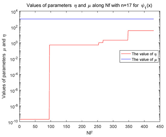
Figure 1. Values of $\eta$ and $\mu$ in function ${\psi }_1\left(x\right)$ with $N=17$ in exact case.

Next, inexact data are referred and we consider the cases of random noises for function value and subgradient. We introduce two kinds of random noises in matlab codes. The first case is ${\theta }_j=0.01\ast normrnd(0,0.1)$, and ${\epsilon }_j=0.01\ast normrd(0,0.1,1,dim)$. The code $normrnd(0,0.1,1,dim)$ generates random numbers from the normal distribution with mean value 0, standard deviation 0.1 and scalars $dim$ and 1 are the row and column dimensions. We take $m_1=0.01$, $\kappa =0.9$, $\gamma =2$, $\tau =2$, $M_0=5$ and $R_0=1000$ in this random error case. The algorithm stops when $V_k\le Tol$ holds or the number of function evaluated is over 1000. The numerical results for this case are report in Table 4.

Table 4. The numerical results of Algorithm 1 for ${\psi }_1\left(x\right)$ and ${\psi }_2\left(x\right)$ in normal case.

	Algorithm 1 for ${\mathit{\psi }}_1\left(\mathit{x}\right)$						Algorithm 1 for ${\mathit{\psi }}_2\left(\mathit{x}\right)$
Dim	Nu	NS	NNA	NF	${\mathit{V}}_{\mathit{k}}$	fk	Nu	NS	NNA	NF	${\mathit{V}}_{\mathit{k}}$	fk
1	5	10	114	130	9.0344$\times {10}^{-7}$	7.0717$\times {10}^{-4}$	1	0	68	70	9.6383$\times {10}^{-7}$	0.49979
2	5	117	126	249	9.2468$\times {10}^{-7}$	3.8879$\times {10}^{-4}$	0	146	82	229	9.7514$\times {10}^{-7}$	1.5986$\times {10}^{-3}$
3	1	89	102	193	9.1171$\times {10}^{-7}$	3.4264$\times {10}^{-4}$	1	83	133	218	9.8973$\times {10}^{-7}$	3.1147$\times {10}^{-5}$
4	1	59	114	175	9.5976$\times {10}^{-7}$	6.5193$\times {10}^{-4}$	1	61	98	161	9.2704$\times {10}^{-7}$	3.3729$\times {10}^{-5}$
5	3	48	87	139	9.4254$\times {10}^{-7}$	7.6518$\times {10}^{-4}$	2	48	107	158	9.9754$\times {10}^{-7}$	7.9746$\times {10}^{-4}$
6	1	44	112	158	9.0774$\times {10}^{-7}$	4.7392$\times {10}^{-4}$	1	43	111	156	9.7216$\times {10}^{-7}$	7.3592$\times {10}^{-4}$
7	3	45	58	107	5.8879$\times {10}^{-7}$	1.5267$\times {10}^{-4}$	3	41	112	157	9.4994$\times {10}^{-7}$	5.6870$\times {10}^{-4}$
8	3	41	98	143	9.3921$\times {10}^{-7}$	6.9636$\times {10}^{-5}$	6	39	116	162	9.4767$\times {10}^{-7}$	1.4089$\times {10}^{-3}$
9	4	41	121	167	9.0501$\times {10}^{-7}$	9.1557$\times {10}^{-3}$	3	36	132	172	9.7158$\times {10}^{-7}$	1.6736$\times {10}^{-2}$
10	5	39	114	159	9.2367$\times {10}^{-7}$	5.4923$\times {10}^{-3}$	3	36	143	183	9.6403$\times {10}^{-7}$	9.3759$\times {10}^{-3}$
11	5	36	106	148	9.3682$\times {10}^{-7}$	1.1568$\times {10}^{-3}$	3	38	139	181	8.4584$\times {10}^{-7}$	3.0633$\times {10}^{-2}$
12	13	39	127	180	9.2902$\times {10}^{-7}$	9.2985$\times {10}^{-3}$	3	36	156	196	9.4762$\times {10}^{-7}$	3.8106$\times {10}^{-2}$
13	15	41	116	173	8.3068$\times {10}^{-7}$	1.4001$\times {10}^{-3}$	6	45	114	166	9.7425$\times {10}^{-7}$	2.8040$\times {10}^{-3}$
14	1	40	110	152	9.2798$\times {10}^{-7}$	3.8884$\times {10}^{-2}$	3	38	145	187	9.5111$\times {10}^{-7}$	1.0486$\times {10}^{-2}$
15	3	39	144	187	9.6793$\times {10}^{-7}$	6.1932$\times {10}^{-2}$	2	35	149	187	9.6589$\times {10}^{-7}$	4.3316$\times {10}^{-2}$
16	15	48	110	174	8.5188$\times {10}^{-7}$	1.7622$\times {10}^{-3}$	21	41	127	190	9.1613$\times {10}^{-7}$	2.7225$\times {10}^{-3}$
17	7	41	127	176	8.9836$\times {10}^{-7}$	6.3638$\times {10}^{-2}$	6	36	167	210	9.2330$\times {10}^{-7}$	3.8989$\times {10}^{-2}$
18	22	38	148	209	9.3322$\times {10}^{-7}$	1.7141$\times {10}^{-1}$	9	37	139	186	9.8447$\times {10}^{-7}$	5.9524$\times {10}^{-2}$
19	44	64	236	345	9.9961$\times {10}^{-7}$	2.3553$\times {10}^{-3}$	159	47	975	1164	9.5532$\times {10}^{-7}$	2.2285$\times {10}^{-3}$
20	35	53	111	200	9.7534$\times {10}^{-7}$	9.3607$\times {10}^{-3}$	31	51	130	213	9.0064$\times {10}^{-7}$	5.1422$\times {10}^{-2}$

From Table 4, we have Algorithm 1 can solve ${\psi }_1\left(x\right)$ and ${\psi }_2\left(x\right)$ successfully for random errors in a reasonable accuracy. We also focus on the parameters $\eta$ and $\mu$ in the implementation of Algorithm 1. Although the convexification parameter ${\eta }_n$ eventually keeps unchanged, the update strategy of the proximal parameter ${\mu }_n$ is complicated. When the noise management step occurs, parameter ${\mu }_n$ is decreasing to reduce the ’noise’ errors’ impact. When the unacceptable condition happens, we increase the parameter ${\mu }_n$ to get a smaller step length. Figure 2 shows the variation of parameters $\eta$ and $\mu$ along NF for ${\psi }_1\left(x\right)$ with $N=19$ in normal random error case.

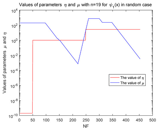
Figure 2. The values of $\eta$ and $\mu$ in function ${\psi }_1\left(x\right)$ with $N=19$ in inexact case.

In the following, we introduce the error case of ${\theta }_j=0.01\ast unifrnd(0,1)$ and ${\epsilon }_j=0.01\ast unifrnd$$(0,1,1,dim)$. The code $unifrnd(0,1,1,dim)$ gives a similar case with the ‘normrd’ case. In this case, we adopt two $Tol$ values and two initial proximal parameter values $R_0$ for different dimension of the variables. Concretely, we take $m_1=0.01$, $\kappa =0.9$, $\tau =2$, $\gamma =2$, $M_0=5$ and $R_0=20$, $Tol={10}^{-6}$ for $N\in \{1,2,\cdots ,8\}$. For $N\in \{9,10,\cdots ,19,20\}$, we take $R_0=200$, $Tol={10}^{-4}$ and the other parameters keep unchanged. We also take 1000 as the upper limit of function evaluated. The algorithm stops when $V_k\le Tol$ holds or the number of function evaluated is over 1000. The numerical results for this error case are reported in Table 5.

Table 5. The numerical results of Algorithm 1 for ${\psi }_1\left(x\right)$ and ${\psi }_2\left(x\right)$ in unifrnd error case.

	Algorithm 1 for ${\mathit{\psi }}_1\left(\mathit{x}\right)$						Algorithm 1 for ${\mathit{\psi }}_2\left(\mathit{x}\right)$
Dim	Nu	NS	NNA	NF	${\mathit{V}}_{\mathit{k}}$	fk	Nu	NS	NNA	NF	${\mathit{V}}_{\mathit{k}}$	fk
1	4	9	83	97	9.0613$\times {10}^{-7}$	−6.4794$\times {10}^{-3}$	2	0	19	22	9.7755$\times {10}^{-7}$	4.9060$\times {10}^{-1}$
2	3	17	127	148	9.1482$\times {10}^{-7}$	−1.8758$\times {10}^{-4}$	1	18	79	99	9.0223$\times {10}^{-7}$	7.7941$\times {10}^{-4}$
3	3	11	110	125	9.0388$\times {10}^{-7}$	1.7436$\times {10}^{-7}$	2	11	83	97	9.5395$\times {10}^{-7}$	−7.1758$\times {10}^{-4}$
4	2	11	79	93	9.4813$\times {10}^{-7}$	7.1079$\times {10}^{-4}$	0	10	81	92	9.4233$\times {10}^{-7}$	2.0590$\times {10}^{-3}$
5	1	10	96	108	9.4407$\times {10}^{-7}$	−4.5471$\times {10}^{-4}$	3	8	102	114	9.0188$\times {10}^{-7}$	6.8412$\times {10}^{-3}$
6	4	11	102	118	9.9976$\times {10}^{-7}$	7.3570$\times {10}^{-3}$	3	13	72	89	9.4247$\times {10}^{-7}$	6.0276$\times {10}^{-3}$
7	6	10	112	129	9.2399$\times {10}^{-7}$	7.5234$\times {10}^{-2}$	7	9	85	102	9.2723$\times {10}^{-7}$	1.2366$\times {10}^{-3}$
8	7	16	108	132	9.7060$\times {10}^{-7}$	1.4824$\times {10}^{-2}$	6	13	102	122	9.1341$\times {10}^{-7}$	7.7913$\times {10}^{-3}$
9	5	38	81	125	9.3352$\times {10}^{-5}$	5.2611$\times {10}^{-4}$	2	36	108	147	9.0509$\times {10}^{-5}$	1.4101$\times {10}^{-2}$
10	7	36	94	138	9.3808$\times {10}^{-5}$	2.7920$\times {10}^{-3}$	2	36	107	146	9.9270$\times {10}^{-5}$	2.3615$\times {10}^{-2}$
11	4	36	125	166	9.3952$\times {10}^{-5}$	6.2396$\times {10}^{-4}$	2	34	142	179	9.7926$\times {10}^{-5}$	2.2681$\times {10}^{-2}$
12	32	39	249	321	9.8977$\times {10}^{-5}$	1.1030$\times {10}^{-3}$	2	34	96	133	9.9074$\times {10}^{-5}$	1.3646$\times {10}^{-2}$
13	7	36	93	137	9.0263$\times {10}^{-5}$	3.8576$\times {10}^{-2}$	6	34	103	144	9.7738$\times {10}^{-5}$	4.7721$\times {10}^{-2}$
14	31	41	231	304	9.6781$\times {10}^{-5}$	4.2488$\times {10}^{-3}$	0	40	83	124	9.6485$\times {10}^{-5}$	7.3474$\times {10}^{-3}$
15	2	38	110	151	9.5999$\times {10}^{-5}$	6.1932$\times {10}^{-2}$	7	34	104	146	9.4630$\times {10}^{-5}$	4.2409$\times {10}^{-2}$
16	5	37	92	135	8.6662$\times {10}^{-5}$	4.9052$\times {10}^{-2}$	6	34	106	147	9.4022$\times {10}^{-5}$	1.1794$\times {10}^{-1}$
17	24	46	205	276	9.5651$\times {10}^{-5}$	−8.0278$\times {10}^{-4}$	4	34	116	155	9.9456$\times {10}^{-5}$	5.7203$\times {10}^{-2}$
18	32	42	217	292	9.4322$\times {10}^{-5}$	1.4177$\times {10}^{-3}$	4	33	107	145	9.0805$\times {10}^{-5}$	5.2319$\times {10}^{-2}$
19	12	38	123	174	9.7789$\times {10}^{-5}$	1.1508$\times {10}^{-1}$	5	35	126	167	9.2005$\times {10}^{-5}$	2.8864$\times {10}^{-1}$
20	24	52	118	195	9.8336$\times {10}^{-5}$	7.6241$\times {10}^{-3}$	21	44	85	151	9.3581$\times {10}^{-5}$	9.4419$\times {10}^{-2}$

From Table 5, Algorithm 1 can solve ${\psi }_1\left(x\right)$ and ${\psi }_2\left(x\right)$ in a reasonable accuracy for the ‘unifrnd’ random error case. In this inexact case, we also illustrate the vary of ${\eta }_n$ and ${\mu }_n$ in Figure 3 and Figure 4. The parameter ${\eta }_n$ is eventually stable. Although the vary of the proximal parameter ${\mu }_n$ is complicate for inexact case, the hypothesis about the upper limits for ${\mu }_n$ in the numerical experiment is reasonable, which are illustrated in the numerical testing.

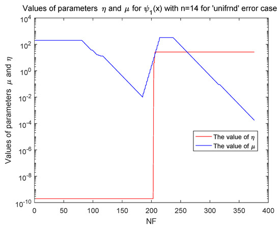
Figure 3. Values of $\eta$ and $\mu$ in function ${\psi }_1\left(x\right)$ with $N=14$ in unifrnd error case.

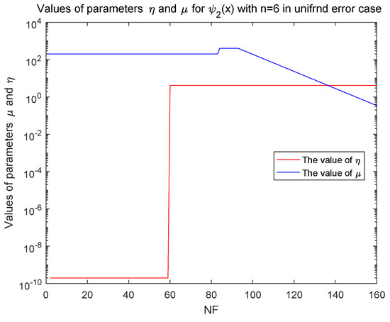
Figure 4. Values of $\eta$ and $\mu$ in function ${\psi }_2\left(x\right)$ with $N=6$ in unifrnd error case.

5.2. Noise’s Impact on Solution Accturacy

The error have different types. To analysis the impact of different noise types, we test five different types of inexact oracles:

• NNE (no noise error): in this case, $\overline{\theta }=\overline{\epsilon }=0$ and ${\theta }_i={\epsilon }_i=0$ for all i in iterative process;
• CNE (constant noise error): in this case, $\overline{\theta }=\overline{\epsilon }={\theta }_i={\epsilon }_i=0.01$, for all i in iterative process;
• VNE (vanishing noise error): in this case, $\overline{\theta }=\overline{\epsilon }=0.01$ and ${\theta }_i={\epsilon }_i=min\{0.01,\parallel x^i\parallel /100\}$ for all i in iterative process;
• CGNE (constant subgradient noise error): in this case, $\overline{\theta }={\theta }_i=0$ and $\overline{\epsilon }={\epsilon }_i=0.01$ for all i in iterative process;
• VGNE (vanishing subgradient noise error): in this case, we set $\overline{\theta }={\theta }_i=0$ and $\overline{\epsilon }=0.01$, ${\epsilon }_i=min\{0.01,\parallel x^i\parallel /100\}$ for all i in iterative process;

In the numerical experiment, the parameters involved are the same with that in the ‘unifrnd’ error case. We present the numerical results of no noise error case (exact values case) in Table 6. In the test, for $N=2$, we take $Tol={10}^{-5}$. In exact case, the number of $NNA$ is always 0, then we omit the columns of $NNA$ in Table 6.

Table 6. The numerical results of Algorithm 1 for ${\psi }_1\left(x\right)$ and ${\psi }_2\left(x\right)$ in NNE case.

	Algorithm 1 for ${\mathit{\psi }}_1\left(\mathit{x}\right)$					Algorithm 1 for ${\mathit{\psi }}_2\left(\mathit{x}\right)$
Dim	Nu	NS	NF	${\mathit{V}}_{\mathit{k}}$	fk	Nu	NS	NF	${\mathit{V}}_{\mathit{k}}$	fk
1	5	61	67	9.4215$\times {10}^{-7}$	4.5882$\times {10}^{-8}$	3	0	4	3.4441$\times {10}^{-9}$	0.5000
2	216	42	259	9.6560$\times {10}^{-7}$	3.7064$\times {10}^{-8}$	7	22	30	4.1491$\times {10}^{-7}$	1.3116$\times {10}^{-8}$
3	19	19	39	5.1917$\times {10}^{-7}$	7.2127$\times {10}^{-8}$	9	15	25	5.2048$\times {10}^{-7}$	8.5245$\times {10}^{-9}$
4	8	21	30	9.6471$\times {10}^{-7}$	6.1925$\times {10}^{-8}$	5	15	21	2.8717$\times {10}^{-7}$	6.8710$\times {10}^{-8}$
5	34	23	58	8.2690$\times {10}^{-7}$	1.3192$\times {10}^{-7}$	16	14	31	4.6146$\times {10}^{-7}$	7.9665$\times {10}^{-8}$
6	52	26	79	7.6472$\times {10}^{-7}$	1.4489$\times {10}^{-7}$	20	18	39	9.7512$\times {10}^{-7}$	2.9449$\times {10}^{-7}$
7	43	29	73	8.2491$\times {10}^{-7}$	1.2567$\times {10}^{-7}$	130	32	163	9.8973$\times {10}^{-7}$	2.6066$\times {10}^{-7}$
8	166	28	195	6.2295$\times {10}^{-7}$	8.9061$\times {10}^{-8}$	66	32	99	6.8694$\times {10}^{-7}$	7.3557$\times {10}^{-8}$
9	64	59	124	9.4850$\times {10}^{-5}$	2.1974$\times {10}^{-5}$	7	67	75	6.2759$\times {10}^{-5}$	1.1151$\times {10}^{-6}$
10	11	55	67	6.9491$\times {10}^{-5}$	1.6440$\times {10}^{-6}$	14	56	71	5.7784$\times {10}^{-5}$	2.3212$\times {10}^{-6}$
11	71	52	124	7.3334$\times {10}^{-5}$	2.9259$\times {10}^{-5}$	8	54	63	9.3601$\times {10}^{-5}$	1.7999$\times {10}^{-6}$
12	180	77	258	5.6646$\times {10}^{-5}$	4.7089$\times {10}^{-6}$	28	57	86	9.4441$\times {10}^{-5}$	1.4864$\times {10}^{-6}$
13	35	76	112	7.8602$\times {10}^{-5}$	2.9328$\times {10}^{-6}$	18	51	70	8.3528$\times {10}^{-5}$	1.7982$\times {10}^{-6}$
14	25	69	95	6.8130$\times {10}^{-5}$	1.9605$\times {10}^{-6}$	28	69	98	8.9934$\times {10}^{-5}$	3.2136$\times {10}^{-6}$
15	111	88	200	9.1881$\times {10}^{-5}$	2.6398$\times {10}^{-6}$	72	68	141	6.7125$\times {10}^{-5}$	6.2161$\times {10}^{-5}$
16	77	82	140	7.7113$\times {10}^{-5}$	2.0920$\times {10}^{-6}$	19	60	80	5.4267$\times {10}^{-5}$	2.4310$\times {10}^{-6}$
17	140	85	226	6.3321$\times {10}^{-5}$	4.4485$\times {10}^{-6}$	25	67	93	6.5668$\times {10}^{-5}$	2.6549$\times {10}^{-6}$
18	698	139	838	8.1746$\times {10}^{-5}$	4.1455$\times {10}^{-6}$	25	56	82	7.2642$\times {10}^{-5}$	2.4928$\times {10}^{-6}$
19	97	109	207	8.5362$\times {10}^{-5}$	2.1782$\times {10}^{-6}$	241	125	367	9.9203$\times {10}^{-5}$	5.6158$\times {10}^{-6}$
20	241	100	342	5.8432$\times {10}^{-5}$	6.6563$\times {10}^{-3}$	85	116	202	9.3362$\times {10}^{-5}$	3.3206$\times {10}^{-6}$

In the following, we present the numerical results of constant noise error case in Table 7. The parameters are same with that in the NNE case except that for ${\psi }_1\left(x\right)$ with $N=2,18$. For the case of ${\psi }_1\left(x\right)$ with $N=2$, we take $Tol={10}^{-1}$, $R_0=200$ and the other parameters keep unchanged. For the case of ${\psi }_1\left(x\right)$ with $N=18$, we take $Tol={10}^0$, $R_0=200$ and the other parameters keep unchanged.

Table 7. The numerical results of Algorithm 1 for ${\psi }_1\left(x\right)$ and ${\psi }_2\left(x\right)$ in CNE case.

	Algorithm 1 for ${\mathit{\psi }}_1\left(\mathit{x}\right)$						Algorithm 1 for ${\mathit{\psi }}_2\left(\mathit{x}\right)$
Dim	Nu	NS	NNA	NF	${\mathit{V}}_{\mathit{k}}$	fk	Nu	NS	NNA	NF	${\mathit{V}}_{\mathit{k}}$	fk
1	2	61	10	74	5.4925$\times {10}^{-7}$	−9.9999$\times {10}^{-3}$	2	0	20	23	9.2963$\times {10}^{-7}$	0.4900
2	$0^{*}$	220	0	221	9.8078$\times {10}^{-2}$	−9.1205$\times {10}^{-3}$	21	23	34	79	9.6577$\times {10}^{-7}$	−9.7816$\times {10}^{-3}$
3	2	13	62	78	9.9421$\times {10}^{-7}$	−9.9472$\times {10}^{-3}$	1	14	43	59	9.6385$\times {10}^{-7}$	−9.9870$\times {10}^{-3}$
4	2	12	42	57	9.0680$\times {10}^{-7}$	−9.3250$\times {10}^{-3}$	2	16	45	64	9.0853$\times {10}^{-7}$	−9.9870$\times {10}^{-3}$
5	5	15	10	31	9.2336$\times {10}^{-7}$	−9.5349$\times {10}^{-3}$	3	12	38	54	9.9726$\times {10}^{-7}$	−3.2581$\times {10}^{-3}$
6	16	23	27	67	8.4599$\times {10}^{-7}$	−9.9969$\times {10}^{-3}$	3	14	98	116	9.5355$\times {10}^{-7}$	−5.3995$\times {10}^{-4}$
7	166	52	28	247	8.6648$\times {10}^{-7}$	−9.9959$\times {10}^{-3}$	8	9	88	106	9.6388$\times {10}^{-7}$	−3.8179$\times {10}^{-3}$
8	11	27	35	74	9.6865$\times {10}^{-7}$	−9.9902$\times {10}^{-3}$	4	13	110	128	9.8178$\times {10}^{-7}$	4.4799$\times {10}^{-3}$
9	10	56	0	73	9.7410$\times {10}^{-5}$	−9.9957$\times {10}^{-3}$	3	63	52	119	8.6710$\times {10}^{-5}$	−9.5796$\times {10}^{-3}$
10	76	84	0	161	9.6288$\times {10}^{-5}$	−9.9981$\times {10}^{-3}$	8	59	58	126	9.7235$\times {10}^{-5}$	−9.3007$\times {10}^{-3}$
11	47	69	0	117	8.3545$\times {10}^{-5}$	−9.9963$\times {10}^{-3}$	8	55	31	95	9.8103$\times {10}^{-5}$	−9.9510$\times {10}^{-3}$
12	338	105	0	444	7.3700$\times {10}^{-5}$	−9.9979$\times {10}^{-3}$	7	44	43	95	9.6506$\times {10}^{-5}$	−9.9432$\times {10}^{-3}$
13	52	93	0	146	6.3101$\times {10}^{-5}$	−9.9978$\times {10}^{-3}$	6	49	59	115	9.8502$\times {10}^{-5}$	−9.1591$\times {10}^{-3}$
14	173	82	0	256	7.8317$\times {10}^{-5}$	−9.9973$\times {10}^{-3}$	12	50	41	104	9.3526$\times {10}^{-5}$	−9.7982$\times {10}^{-3}$
15	28	71	34	134	9.1862$\times {10}^{-5}$	−9.8835$\times {10}^{-3}$	42	69	58	170	9.4662$\times {10}^{-5}$	−8.7053$\times {10}^{-3}$
16	34	70	0	105	7.4213$\times {10}^{-5}$	−9.9973$\times {10}^{-3}$	9	56	87	153	9.0649$\times {10}^{-5}$	−5.9286$\times {10}^{-3}$
17	104	95	0	200	6.0123$\times {10}^{-5}$	−9.9970$\times {10}^{-3}$	16	50	69	136	9.0611$\times {10}^{-5}$	−7.4826$\times {10}^{-3}$
18	$3^{*}$	62	0	66	9.9386$\times {10}^{-1}$	5.1193$\times {10}^{-2}$	8	52	74	135	9.3028$\times {10}^{-5}$	−1.9240$\times {10}^{-3}$
19	93	109	0	203	9.9699$\times {10}^{-5}$	−9.9977$\times {10}^{-3}$	12	34	104	151	9.3323$\times {10}^{-5}$	2.8573$\times {10}^{-1}$
20	44	70	0	115	5.8482$\times {10}^{-5}$	−3.3485$\times {10}^{-3}$	19	76	98	194	9.3637$\times {10}^{-5}$	−3.0299$\times {10}^{-4}$

Next, Table 8 presents the results for the vanishing noise error case. The parameters keep unchanged except that for ${\psi }_1\left(x\right)$ with $N=2$ and ${\psi }_2\left(x\right)$ with $N=8$. In the case of ${\psi }_1\left(x\right)$ with $N=2$, we take $TOL={10}^{-1}$ and the other parameters keep unchanged. For the ${\psi }_2\left(x\right)$ with $N=8$ case, we take $R_0=10$ and other parameters keep unchanged. It also should note the results for the case of ${\psi }_2\left(x\right)$ with $N=19$.

Table 8. The numerical results of Algorithm 1 for ${\psi }_1\left(x\right)$ and ${\psi }_2\left(x\right)$ in VNE case.

	Algorithm 1 for ${\mathit{\psi }}_1\left(\mathit{x}\right)$						Algorithm 1 for ${\mathit{\psi }}_2\left(\mathit{x}\right)$
Dim	Nu	NS	NNA	NF	${\mathit{V}}_{\mathit{k}}$	fk	Nu	NS	NNA	NF	${\mathit{V}}_{\mathit{k}}$	fk
1	3	63	0	67	2.2411$\times {10}^{-7}$	3.7773$\times {10}^{-9}$	1	0	90	92	9.4261$\times {10}^{-7}$	0.4900
2	1 ${}^{*}$	27	0	29	9.8574$\times {10}^{-2}$	9.6203$\times {10}^{-4}$	14	23	0	38	4.1976$\times {10}^{-7}$	2.1736$\times {10}^{-8}$
3	4	18	0	23	8.8275$\times {10}^{-7}$	1.3800$\times {10}^{-8}$	5	15	0	21	4.5675$\times {10}^{-7}$	6.2853$\times {10}^{-8}$
4	6	20	0	27	5.7581$\times {10}^{-7}$	3.5958$\times {10}^{-8}$	16	20	0	37	3.7227$\times {10}^{-7}$	4.9713$\times {10}^{-8}$
5	45	32	0	78	5.6445$\times {10}^{-7}$	1.0097$\times {10}^{-7}$	16	20	0	37	9.0282$\times {10}^{-7}$	1.6974$\times {10}^{-7}$
6	11	22	0	34	8.8817$\times {10}^{-7}$	1.0183$\times {10}^{-7}$	34	25	0	60	6.8176$\times {10}^{-7}$	6.3339$\times {10}^{-8}$
7	11	17	45	74	9.7074$\times {10}^{-7}$	8.0881$\times {10}^{-2}$	71	33	0	105	9.2437$\times {10}^{-7}$	9.3392$\times {10}^{-8}$
8	88	44	11	144	5.7791$\times {10}^{-7}$	2.4473$\times {10}^{-7}$	3 ${}^{*}$	16	121	141	9.7224$\times {10}^{-7}$	3.5503$\times {10}^{-2}$
9	26	72	9	108	4.9732$\times {10}^{-5}$	2.4391$\times {10}^{-6}$	20	59	0	80	7.8092$\times {10}^{-5}$	2.8594$\times {10}^{-6}$
10	72	85	0	158	9.9915$\times {10}^{-5}$	2.2020$\times {10}^{-6}$	14	54	0	69	8.7709$\times {10}^{-5}$	4.8392$\times {10}^{-6}$
11	91	80	0	172	9.4444$\times {10}^{-5}$	1.7418$\times {10}^{-6}$	21	64	0	86	5.3167$\times {10}^{-5}$	1.8802$\times {10}^{-6}$
12	252	97	3	353	6.2931$\times {10}^{-5}$	3.9407$\times {10}^{-6}$	96	78	0	175	8.7760$\times {10}^{-5}$	3.1215$\times {10}^{-6}$
13	39	75	6	121	9.2734$\times {10}^{-5}$	4.3186$\times {10}^{-6}$	17	51	0	69	7.3807$\times {10}^{-5}$	1.7909$\times {10}^{-6}$
14	391	98	5	495	9.6182$\times {10}^{-5}$	5.7300$\times {10}^{-6}$	22	59	0	82	9.4783$\times {10}^{-5}$	3.1236$\times {10}^{-6}$
15	75	105	0	181	9.7263$\times {10}^{-5}$	2.3624$\times {10}^{-5}$	290	85	0	376	3.9385$\times {10}^{-5}$	4.0266$\times {10}^{-6}$
16	25	55	0	81	9.2934$\times {10}^{-5}$	2.9491$\times {10}^{-6}$	20	61	0	82	7.7500$\times {10}^{-5}$	2.9207$\times {10}^{-6}$
17	62	80	6	149	6.7672$\times {10}^{-5}$	5.1710$\times {10}^{-6}$	35	57	0	93	9.9252$\times {10}^{-5}$	1.7155$\times {10}^{-6}$
18	203	138	8	350	6.5785$\times {10}^{-5}$	4.5494$\times {10}^{-6}$	25	52	0	78	6.6201$\times {10}^{-5}$	1.8421$\times {10}^{-6}$
19	88	96	2	187	8.7263$\times {10}^{-5}$	4.5004$\times {10}^{-6}$	46	401	120	567	3.6082$\times {10}^{12}$ ${}^{*}$	1.7001$\times {10}^{-3}$
20	140	91	2	234	6.5071$\times {10}^{-5}$	5.5017$\times {10}^{-3}$	23	94	63	181	9.3351$\times {10}^{-5}$	7.6290$\times {10}^{-4}$

In the following, Table 9 presents the results for the constant subgradient noise error case (CGNE). The parameters keep unchanged except the case of ${\psi }_1\left(x\right)$ with $N=18$. In this case, we take $Tol={10}^0$ and $R_0=500$. Table 10 presents the results for the vanishing subgradient noise error case (VGNE). The parameters keep unchanged except the cases of ${\psi }_1\left(x\right)$ with $N=2,7,14,18$. In these cases, we take $Tol={10}^{-1},R_0=200$ and other parameters keep unchanged.

Table 9. The numerical results of Algorithm 1 for ${\psi }_1\left(x\right)$ and ${\psi }_2\left(x\right)$ in CGNE case.

	Algorithm 1 for ${\mathit{\psi }}_1\left(\mathit{x}\right)$						Algorithm 1 for ${\mathit{\psi }}_2\left(\mathit{x}\right)$
Dim	Nu	NS	NNA	NF	${\mathit{V}}_{\mathit{k}}$	fk	Nu	NS	NNA	NF	${\mathit{V}}_{\mathit{k}}$	fk
1	2	61	10	74	5.4925$\times {10}^{-7}$	1.3472$\times {10}^{-7}$	2	0	20	23	9.2963$\times {10}^{-7}$	0.5000
2	215	31	90	337	4.3225$\times {10}^{-7}$	7.1521$\times {10}^{-7}$	21	23	34	79	9.6577$\times {10}^{-7}$	2.1843$\times {10}^{-4}$
3	2	13	62	78	9.9421$\times {10}^{-7}$	5.2650$\times {10}^{-5}$	1	14	43	59	9.6385$\times {10}^{-7}$	1.2983$\times {10}^{-5}$
4	2	12	42	57	9.0680$\times {10}^{-7}$	6.7504$\times {10}^{-4}$	2	16	45	64	9.0853$\times {10}^{-7}$	1.1792$\times {10}^{-5}$
5	5	15	10	31	9.2336$\times {10}^{-7}$	4.6506$\times {10}^{-4}$	3	12	38	54	9.9726$\times {10}^{-7}$	6.7418$\times {10}^{-3}$
6	16	23	27	67	8.4599$\times {10}^{-7}$	3.1286$\times {10}^{-6}$	3	14	98	116	9.5355$\times {10}^{-7}$	9.4601$\times {10}^{-3}$
7	162	53	23	239	7.8402$\times {10}^{-7}$	2.3823$\times {10}^{-6}$	8	9	88	106	9.6388$\times {10}^{-7}$	6.1821$\times {10}^{-3}$
8	11	27	35	74	9.6865$\times {10}^{-7}$	9.8010$\times {10}^{-6}$	4	13	110	128	9.8178$\times {10}^{-7}$	1.4480$\times {10}^{-2}$
9	10	56	6	73	9.7410$\times {10}^{-5}$	4.2731$\times {10}^{-6}$	3	63	52	119	8.6710$\times {10}^{-5}$	4.2042$\times {10}^{-4}$
10	76	84	0	161	9.6289$\times {10}^{-5}$	1.9282$\times {10}^{-6}$	8	59	58	126	9.7235$\times {10}^{-5}$	6.9928$\times {10}^{-4}$
11	47	69	0	117	8.3546$\times {10}^{-5}$	3.7396$\times {10}^{-6}$	8	55	31	95	9.8103$\times {10}^{-5}$	4.9014$\times {10}^{-5}$
12	363	104	0	468	9.4169$\times {10}^{-5}$	2.6927$\times {10}^{-6}$	7	44	43	95	9.6506$\times {10}^{-5}$	5.6826$\times {10}^{-5}$
13	52	93	0	146	6.3104$\times {10}^{-5}$	2.1522$\times {10}^{-6}$	6	49	59	115	9.8502$\times {10}^{-5}$	8.4093$\times {10}^{-4}$
14	173	82	0	256	7.8317$\times {10}^{-5}$	2.7201$\times {10}^{-6}$	12	50	41	104	9.3526$\times {10}^{-5}$	2.0185$\times {10}^{-5}$
15	28	71	34	134	9.1862$\times {10}^{-5}$	1.1654$\times {10}^{-4}$	42	69	58	170	9.4662$\times {10}^{-5}$	1.2947$\times {10}^{-3}$
16	34	70	0	105	7.4213$\times {10}^{-5}$	2.6541$\times {10}^{-6}$	9	56	87	153	9.0649$\times {10}^{-5}$	4.0714$\times {10}^{-3}$
17	104	95	0	200	6.0123$\times {10}^{-5}$	3.0115$\times {10}^{-3}$	16	50	69	136	9.0611$\times {10}^{-5}$	2.5174$\times {10}^{-3}$
18	2 ${}^{*}$	77	0	80	8.0272$\times {10}^{-1}$	3.3133$\times {10}^{-2}$	8	52	74	135	9.3028$\times {10}^{-5}$	8.0760$\times {10}^{-3}$
19	74	109	0	184	9.9172$\times {10}^{-5}$	2.6683$\times {10}^{-6}$	12	34	104	151	9.3323$\times {10}^{-5}$	2.9573$\times {10}^{-1}$
20	44	70	0	115	5.8482$\times {10}^{-5}$	6.6515$\times {10}^{-3}$	19	76	101	197	9.8115$\times {10}^{-5}$	9.6949$\times {10}^{-3}$

Table 10. The numerical results of Algorithm 1 for ${\psi }_1\left(x\right)$ and ${\psi }_2\left(x\right)$ in VGNE case.

	Algorithm 1 for ${\mathit{\psi }}_1\left(\mathit{x}\right)$						Algorithm 1 for ${\mathit{\psi }}_2\left(\mathit{x}\right)$
Dim	Nu	NS	NNA	NF	${\mathit{V}}_{\mathit{k}}$	fk	Nu	NS	NNA	NF	${\mathit{V}}_{\mathit{k}}$	fk
1	3	63	0	67	4.3452$\times {10}^{-7}$	1.0116$\times {10}^{-8}$	2	0	20	23	9.2964$\times {10}^{-7}$	0.5000
2	27 ${}^{*}$	298	0	326	3.3338$\times {10}^{-2}$	1.1757$\times {10}^{-3}$	18	23	41	83	9.7677$\times {10}^{-7}$	2.7914$\times {10}^{-6}$
3	6	17	0	24	4.6189$\times {10}^{-7}$	4.8693$\times {10}^{-8}$	2	17	2	22	7.6315$\times {10}^{-7}$	1.3123$\times {10}^{-7}$
4	2	20	0	23	3.4081$\times {10}^{-7}$	6.7561$\times {10}^{-8}$	3	15	38	57	9.4155$\times {10}^{-7}$	9.1216$\times {10}^{-6}$
5	32	32	0	65	9.6611$\times {10}^{-7}$	1.3557$\times {10}^{-7}$	5	16	45	67	8.0761$\times {10}^{-7}$	2.2608$\times {10}^{-5}$
6	16	24	0	41	3.8862$\times {10}^{-7}$	9.8845$\times {10}^{-8}$	5	21	58	85	9.2491$\times {10}^{-7}$	2.4062$\times {10}^{-5}$
7	6 ${}^{*}$	57	0	64	2.9199$\times {10}^{-2}$	1.0333$\times {10}^{-5}$	8	20	68	97	9.4552$\times {10}^{-7}$	4.4226$\times {10}^{-3}$
8	130	41	0	172	5.8681$\times {10}^{-7}$	4.3867$\times {10}^{-8}$	7	15	93	116	9.8671$\times {10}^{-7}$	1.0319$\times {10}^{-2}$
9	54	74	0	129	8.5412$\times {10}^{-5}$	2.3582$\times {10}^{-6}$	8	54	19	82	8.9252$\times {10}^{-5}$	1.3088$\times {10}^{-5}$
10	91	79	0	171	6.4727$\times {10}^{-5}$	3.4788$\times {10}^{-6}$	7	51	15	74	7.2476$\times {10}^{-5}$	1.2106$\times {10}^{-5}$
11	79	75	0	155	7.3459$\times {10}^{-5}$	4.7386$\times {10}^{-6}$	6	54	36	97	4.8921$\times {10}^{-5}$	7.0049$\times {10}^{-5}$
12	172	90	0	263	4.2617$\times {10}^{-5}$	3.9532$\times {10}^{-6}$	9	70	39	119	8.9773$\times {10}^{-5}$	1.3272$\times {10}^{-4}$
13	46	78	0	125	8.4436$\times {10}^{-5}$	2.9852$\times {10}^{-6}$	5	50	40	96	9.4999$\times {10}^{-5}$	2.1125$\times {10}^{-4}$
14	8 ${}^{*}$	78	0	87	6.3657$\times {10}^{-2}$	7.5245$\times {10}^{-6}$	14	47	34	96	9.2984$\times {10}^{-5}$	7.1209$\times {10}^{-5}$
15	203	80	0	284	6.9332$\times {10}^{-5}$	1.4201$\times {10}^{-6}$	49	80	54	184	7.2507$\times {10}^{-5}$	3.7361$\times {10}^{-4}$
16	55	63	0	119	6.5930$\times {10}^{-5}$	2.2500$\times {10}^{-6}$	10	52	70	133	9.2583$\times {10}^{-5}$	2.3373$\times {10}^{-3}$
17	79	79	0	159	8.5136$\times {10}^{-5}$	4.5443$\times {10}^{-6}$	24	56	55	136	7.3576$\times {10}^{-5}$	6.2449$\times {10}^{-4}$
18	47 ${}^{*}$	222	16	285	4.4363$\times {10}^{16}$ ${}^{*}$	2.6364$\times {10}^{-2}$	9	47	84	141	9.0335$\times {10}^{-5}$	2.4064$\times {10}^{-3}$
19	54	89	0	144	6.6094$\times {10}^{-5}$	2.5192$\times {10}^{-6}$	308	126	68	503	6.8994$\times {10}^{-5}$	1.0272$\times {10}^{-3}$
20	97	98	0	196	7.8812$\times {10}^{-5}$	6.6541$\times {10}^{-3}$	19	79	72	171	9.1718$\times {10}^{-5}$	6.4603$\times {10}^{-3}$

Next, we compare the numerical performance of different noise type. For comparing the performances, we adopt the formula Precision $=\left|log10\right(\left|fk\right|\left)\right|$ and regard the NNE case as a benchmark for comparison. The cases of constant noise (CNE and CGNE) and exact form (NNE) are referred to in Figure 5. It is clear that the exact case has the best performance and Algorithm 1 can achieve a reasonable accuracy for the constant case. Meanwhile, the performance of CGNE case is better that than of CNE case. Similarly, Figure 6 reports the numerical performance for the vanishing cases (VNE and VGNE) and the exact form (NNE). From Figure 6, the performance of the VGNE case is comparable with that of the exact (NNE) case. Meanwhile, the performance of the vanishing error cases are generally better than that in the constant error cases.

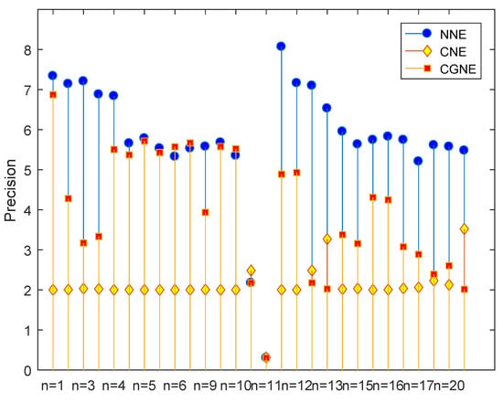
Figure 5. Performance of Algorithm 1 for the NNE, CNE and CGNE cases.

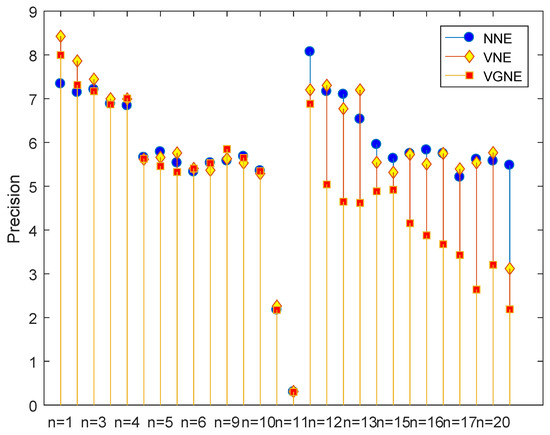
Figure 6. Performance of Algorithm 1 for the NNE, VNE and VGNE cases.

5.3. Application to Some DC Problems

In this subsection, we test some unconstrained DC examples to illustrate the effectiveness of Algorithm 1. These examples come from [42,43,44]. Usually, the DC function has the form: $\psi \left(x\right)=f\left(x\right)-g\left(x\right)$. If we take $h\left(x\right)=-g\left(x\right)$, the problems are in the form of (1).

Problem 1.

Dimension: $N=2$,

Component functions: $f\left(x\right)=|x_1-1|+200max\left\{0,|x_1|-x_2\right\}$; $g\left(x\right)=100\left(|x_1|-x_2\right)$,

Relevant information: $x^0={(2,5)}^T$, $x^{*}={(1,1)}^T$, ${\psi }^{*}=0$.

Problem 2.

Dimension: $N=4$,

Component functions: $f\left(x\right)=|x_1-1|+200max\left\{0,|x_1|-x_2\right\}+180max\left\{0,|x_3|-x_4\right\}+\left|x_3-1\right|+10.1\left(|x_2-1|+|x_4-1|\right)+4.95\left|x_2+x_4-2\right|$; $g\left(x\right)=100\left(|x_1|-x_2\right)+90\left(|x_3|-x_4\right)+4.95\left|x_2-x_4\right|$,

Relevant information: $x^0={(1,3,3,1)}^T$, $x^{*}={(1,1,1,1)}^T$, ${\psi }^{*}=0$.

Problem 3.

Dimension: $N=2,5,10$,

Component functions: $f\left(x\right)=Nmax\left\{\right|x_i|:i=1,\cdots ,N\}$, $g\left(x\right)={\sum }_1^N\left|x_i\right|$,

Relevant information: $x^0={(i,i=1,\cdots ,\lfloor N/2\rfloor ,-i,i=\lfloor N/2\rfloor +1,\cdots ,N)}^T$, $x^{*}={(x_1^{*},\cdots ,x_N^{*})}^T$, $x_i^{*}=a$ or $x_i^{*}=-a$, $a\in \mathbf{R}$, $i=1,\cdots ,N$, ${\psi }^{*}=0$.

Problem 4.

Dimension: $N=4$,

Component functions: $f\left(x\right)=x_1^2+{(x_1-1)}^2+2{(x_1-2)}^2+{(x_1-3)}^2+2x_2^2+{(x_2-1)}^2+2{(x_2-2)}^2+x_3^2+{(x_3-1)}^2+2{(x_3-2)}^2+{(x_3-3)}^2+2x_4^2+{(x_4-1)}^2+2{(x_4-2)}^2$;

$g\left(x\right)=max\{{(x_1-2)}^2+x_2^2,{(x_3-2)}^2+x_4^2\}+max\{{(x_1-2)}^2+{(x_2-1)}^2,{(x_3-2)}^2+{(x_4-1)}^2\}+max\{{(x_1-3)}^2+x_2^2,{(x_3-3)}^2+x_4^2\}+max\{x_1^2+{(x_2-2)}^2,x_3^2+{(x_4-2)}^2\}+max\{{(x_1-1)}^2+{(x_2-2)}^2,{(x_3-1)}^2+{(x_4-2)}^2\},$

Relevant information: $x^0={(3,1,3,1)}^T$, $x^{*}={(7/3,1/3,0.5,2)}^T$, ${\psi }^{*}=11/6$;

Problem 5.

Dimension: $N=2,5$,

Component functions: $f\left(x\right)=20max\left\{\right|{\sum }_{i=1}^N(x_i-x_i^{*})t_j^{i-1}|:j=1,2,\cdots ,20\}$,

$g\left(x\right)={\sum }_{j=1}^{20}\left|{\sum }_{i=1}^N(x_i-x_i^{*})t_j^{i-1}\right|,t_j=0.05j,j=1,2,\cdots ,20,$

Relevant information: $x^0={(1/N,0,\cdots ,0)}^T$, $x^{*}={(1/N,1/N,\cdots ,1/N)}^T$, ${\psi }^{*}=0$.

Problem 6.

Dimension: $N=2,4$,

Component functions: $f\left(x\right)={\sum }_{j=1}^{100}\left|{\sum }_{i=1}^N(x_i-x_i^{*})t_j^{i-1}\right|,t_j=0.01j,j=1,2,\cdots ,100,$

$g\left(x\right)=max\left\{\right|{\sum }_{i=1}^N(x_i-x_i^{*})t_j^{i-1}|:j=1,2,\cdots ,100\}$

Relevant information: $x^0={(0,0,\cdots ,0)}^T$, $x^{*}={(1/N,1/N,\cdots ,1/N)}^T$, ${\psi }^{*}=0$.

For the effectiveness of Algorithm 1, we compare it with the TCM algorithm, NCVX algorithm and penalty NCVX algorithm in [42]. The values of parameters in Algorithm 1 are that: $m_1=0.01$, $\kappa =0.9$, $\tau =2$, $\gamma =2$, $M_0=5$, $R_0=10$ and $Tol={10}^{-3}$. The results can be seen in Table 11. Meanwhile the ∗ in Table 11 means the obtained value is not optimal. From Table 11, we have that Algorithm 1 can successfully solve these DC problems, however the TCM algorithm cannot solve Problem 4, NCVX algorithm cannot solve Problems 1 and 4 and the penalty NCVX algorithm can not solve Problem 1. Then, Algorithm 1 is reliable. From the obtained function value and the number of function evaluations, Algorithm 1 is also effective.

Table 11. The numerical results for Algorithm 1, TCM, NCVX and PNCVX algorithms in Problems 1–5.

		Algorithm 1		TCM		NCVX		PNCVX
Pr	n	Nf	fk	Nf	fk	Nf	fk	Nf	fk	${\mathit{\psi }}^{*}$
1	2	204	7.4219$\times {10}^{-10}$	526	8.4453$\times {10}^{-9}$	20	1.0000 ${}^{*}$	48	1.0000 ${}^{*}$	0
2	4	69	6.4293$\times {10}^{-7}$	517	3.7104$\times {10}^{-9}$	59	6.8183$\times {10}^{-6}$	59	5.2088$\times {10}^{-7}$	0
3	2	6	2.0000$\times {10}^{-11}$	125	4.0552$\times {10}^{-11}$	19	1.2800$\times {10}^{-8}$	4	1.2500$\times {10}^{-7}$	0
3	5	30	3.7100$\times {10}^{-6}$	399	3.6698$\times {10}^{-10}$	25	2.5204$\times {10}^{-5}$	87	7.1731$\times {10}^{-8}$	0
3	10	91	1.4116$\times {10}^{-4}$	844	1.0639$\times {10}^{-9}$	34	6.0636$\times {10}^{-8}$	78	2.2092$\times {10}^{-8}$	0
4	4	21	1.8333	307	9.2000 ${}^{*}$	5	9.2000 ${}^{*}$	34	1.8333	11/6
5	2	32	5.7727$\times {10}^{-6}$	149	1.9922$\times {10}^{-10}$	19	1.1842$\times {10}^{-8}$	24	7.5230$\times {10}^{-9}$	0
5	5	12	4.0654$\times {10}^{-7}$	1174	7.1262$\times {10}^{-10}$	13	9.6573$\times {10}^{-9}$	12	1.1546$\times {10}^{-10}$	0

For the above DC problems, we consider the vanishing noise error (VNE) case and the exact (NNE case. We also take 1000 as the upper limit of function evaluated. The algorithm stops when $V_k\le Tol$ holds or the number of function evaluated is over 1000. For the vanishing noise case, we set ${\theta }_i=min\{0.01,\parallel x-x^{*}\parallel /100\}$ and ${\epsilon }_i=min\{0.01,\parallel x-x^{*}\parallel /100\}$ except Problem 3. In Problem 3, the optimal solutions vary with the dimensions, then we set ${\theta }_i={min\{0.01,\parallel x\parallel }^2/100\}$ and ${\epsilon }_i={min\{0.01,\parallel x\parallel }^2/100\}$. Table 12 presents the results for the vanishing noise error case (VNE) and the exact case (NNE). The column $Pr$ in Table 12 denotes the index of problems. We also compute the Precision. However it is not suitable since the optimal value is not 0. To deal with that, we take $a_k=(fk-f^{*})/f^{*}$ and Precision $=\left|log10\right(\left|a_k\right|\left)\right|$. The numerical results are reported as follows.

Table 12. The numerical results of Algorithm 1 for these DC problems in VNE and NNE cases.

		Algorithm 1 for VNE Case							Algorithm 1 for NNE Case
Pr	Dim	Nu	NS	NNA	NF	${\mathit{V}}_{\mathit{k}}$	fk	Precision	Nu	NS	RS	NF	${\mathit{V}}_{\mathit{k}}$	fk	Precision
1	2	2	199	0	202	7.3309$\times {10}^{-4}$	−9.8726$\times {10}^{-3}$	2.0044	3	200	1	204	1.8221$\times {10}^{-6}$	7.4219$\times {10}^{-10}$	9.1295
2	4	8	68	0	77	7.6724$\times {10}^{-4}$	1.7527$\times {10}^{-6}$	5.7563	5	63	2	69	1.5569$\times {10}^{-5}$	6.4293$\times {10}^{-7}$	6.1918
3	2	1	7	0	9	6.4421$\times {10}^{-5}$	−4.9703$\times {10}^{-3}$	2.3010	0	5	0	6	3.2601$\times {10}^{-8}$	2.0000$\times {10}^{-11}$	10.6990
3	5	307	93	270	671	9.8576$\times {10}^{-4}$	−8.7570$\times {10}^{-3}$	2.0555	1	28	0	30	2.3067$\times {10}^{-5}$	3.7122$\times {10}^{-6}$	5.4304
3	10	6	267	24	298	2.6637$\times {10}^{-4}$	1.1480$\times {10}^{-1}$	0.9401	1	89	0	91	2.9760$\times {10}^{-4}$	1.4116$\times {10}^{-4}$	3.8503
4	4	2	23	0	26	8.2023$\times {10}^{-4}$	1.8234	2.2661	1	19	0	21	8.8458$\times {10}^{-4}$	1.8333	4.7404
5	2	1	6	0	8	6.2198$\times {10}^{-4}$	1.6864$\times {10}^{-4}$	3.7730	6	25	0	32	9.2682$\times {10}^{-4}$	5.7727$\times {10}^{-6}$	5.2386
5	5	5	13	0	19	8.0435$\times {10}^{-4}$	−6.5385$\times {10}^{-4}$	3.1845	2	9	0	12	7.5698$\times {10}^{-4}$	4.0654$\times {10}^{-7}$	6.3909
6	2	2	5	0	8	1.1607$\times {10}^{-4}$	1.8586$\times {10}^{-5}$	4.7308	2	4	2	7	1.0840$\times {10}^{-12}$	5.3857$\times {10}^{-15}$	14.2688
6	4	20	20	113	154	1.3749$\times {10}^{-4}$	−2.6406$\times {10}^{-3}$	2.5850	4	11	2	16	1.3123$\times {10}^{-4}$	1.9301$\times {10}^{-7}$	6.7144

From Table 12, Algorithm 1 can successfully solve the above DC problems in a higher precision and is effective to the VNE case in a reasonable accuracy. Then, Algorithm 1 is effective and reliable to the above DC problems. During the numerical experiment, we also focus on the variation of parameters $\eta$ and $\mu$, which are both bounded and the parameter $\eta$ eventually keeps unchanged, which can be illustrated in Figure 7 and Figure 8.

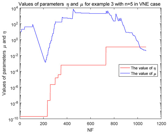
Figure 7. The values of $\eta$ and $\mu$ in Problem 3 with $N=5$ in the VNE case.

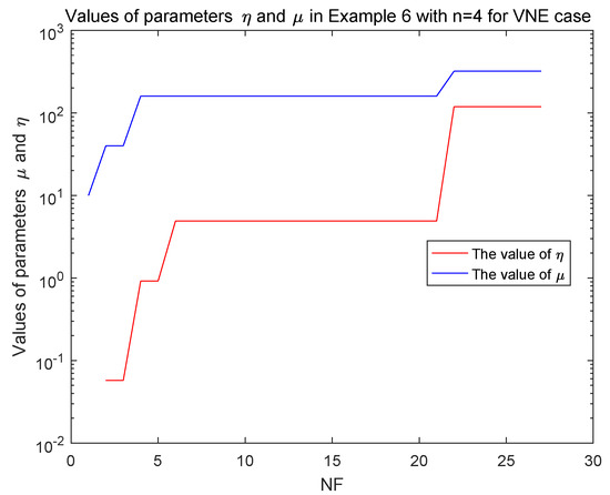
Figure 8. The values of $\eta$ and $\mu$ in Problem 6 with $N=4$ in the VNE case.

6. Conclusions

In this paper, we consider a special class of nonconvex and nonsmooth composite problem. The problem is constituted by the sum of two functions, one is finite convex with inexact information and the other is a nonconvex function (lower-${\mathcal{C}}^2$). For the nonconvex function, we utilize the convexification technique and adjust the parameter dynamically to make sure the linearization errors of the augment function nonnegative and construct the corresponding cutting plane models. Then, we regard the sum of the convex function and the augment function as an approximate function. For the convex function with inexact information, we construct the cutting plane model by its inexact information and notice that the cutting plane model may not be below the convex function. Then, the sum of the cutting plane models of the convex function with inexact information and the augment function is regarded as a cutting plane model of the approximate function. After that, we design an adaptive proximal bundle method. Meanwhile, for the convex function with inexact information, we utilize the noise management strategy and update adaptively the proximal parameter to reduce the influence of inexact information. Two polynomial functions including five different inexact types and six DC problems with different dimension are referred to in the numerical experiment. The preliminary numerical results show our algorithm is interesting and reliable. Meanwhile, our method can also be applied to some constraint problems and stochastic programming in the future.

References

- Condat, L. A primal-dual splitting method for convex optimization involving Lipschitzian, proximable and linear composite terms. J. Optim. Theory Appl. 2013, 158, 460–479. [Google Scholar] [CrossRef]
- Li, G.Y.; Pong, T.K. Global convergence of splitting methods for nonconvex composite optimization. SIAM J. Optim. 2015, 25, 2434–2460. [Google Scholar] [CrossRef]
- Hong, M.; Luo, Z.Q. On the linear convergence of the alternating direction method of multipliers. Math. Program. 2017, 162, 165–199. [Google Scholar] [CrossRef]
- Li, D.; Pang, L.P.; Chen, S. A proximal alternating linearization method for nonconvex optimization problems. Optim. Method Softw. 2014, 29, 771–785. [Google Scholar] [CrossRef]
- Burke, J.V.; Lewis, A.S.; Overton, M.L. A robust gradient sampling algorithm for nonsmooth, nonconvex optimization. SIAM J. Optim. 2005, 15, 751–779. [Google Scholar] [CrossRef]
- Kiwiel, K.C. A method of centers with approximate subgradient linearizations for nonsmooth convex optimization. SIAM J. Optim. 2008, 18, 1467–1489. [Google Scholar] [CrossRef]
- Yuan, G.L.; Meng, Z.H.; Li, Y. A modified Hestenes and Stiefel conjugate gradient algorithm for large-scale nonsmooth minimizations and nonlinear equations. J. Optim. Theory Appl. 2016, 168, 129–152. [Google Scholar] [CrossRef]
- Yuan, G.L.; Sheng, Z. Nonsmooth Optimization Algorithms; Science Press: Beijing, China, 2017. [Google Scholar]
- Yuan, G.L.; Wei, Z.X.; Li, G. A modified Polak-Ribière-Polyak conjugate gradient algorithm for nonsmooth convex programs. J. Comput. Appl. Math. 2014, 255, 86–96. [Google Scholar] [CrossRef]
- Lv, J.; Pang, L.P.; Meng, F.F. A proximal bundle method for constrained nonsmooth nonconvex optimization with inexact information. J. Glob. Optim. 2018, 70, 517–549. [Google Scholar] [CrossRef]
- Yang, Y.; Pang, L.P.; Ma, X.F.; Shen, J. Constrained nonconvex nonsmooth optimization via proximal bundle method. J. Optim. Theory Appl. 2014, 163, 900–925. [Google Scholar] [CrossRef]
- Fuduli, A.; Gaudioso, M.; Giallombardo, G. Minimizing nonconvex nonsmooth functions via cutting planes and proximity control. SIAM J. Optim. 2004, 14, 743–756. [Google Scholar] [CrossRef]
- Sagastizábal, C. Composite proximal bundle method. Math. Program. 2013, 140, 189–233. [Google Scholar] [CrossRef]
- Mäkelä, M.M. Survey of bundle methods for nonsmooth optimization. Optim. Method Softw. 2002, 17, 1–29. [Google Scholar] [CrossRef]
- Hare, W.; Sagastizábal, C.; Solodov, M. A proximal bundle method for nonsmooth nonconvex functions with inexact information. Comput. Optim. Appl. 2016, 63, 1–28. [Google Scholar] [CrossRef]
- Sagastizábal, C.; Hare, W. A redistributed proximal bundle method for nonconvex optimization. SIAM J. Optim. 2010, 20, 2442–2473. [Google Scholar]
- Kiwiel, K.C. A proximal bundle method with approximate subgradient linearizations. SIAM J. Optim. 2006, 16, 1007–1023. [Google Scholar] [CrossRef]
- Kiwiel, K.C. A linearization algorithm for nonsmooth minimization. Math. Oper. Res. 1985, 10, 185–194. [Google Scholar] [CrossRef]
- Tang, C.M.; Liu, S.; Jian, J.B.; Li, J.L. A feasible SQP-GS algorithm for nonconvex, nonsmooth constrained optimization. Numer. Algorithms 2014, 65, 1–22. [Google Scholar] [CrossRef]
- Tang, C.M.; Jian, J.B. Strongly sub-feasible direction method for constrained optimization problems with nonsmooth objective functions. Eur. J. Oper. Res. 2012, 218, 28–37. [Google Scholar] [CrossRef]
- Hintermüller, M. A proximal bundle method based on approximate subgradients. Comput. Optim. Appl. 2001, 20, 245–266. [Google Scholar] [CrossRef]
- Lukšan, L.; Vlček, J. A bundle-Newton method for nonsmooth unconstrained minimization. Math. Program. 1998, 83, 373–391. [Google Scholar] [CrossRef]
- Solodov, M.V. On approximations with finite precision in bundle methods for nonsmooth optimization. J. Optim. Theory Appl. 2003, 119, 151–165. [Google Scholar] [CrossRef]
- Kiwiel, K.C. Restricted step and Levenberg-Marquardt techniques in proximal bundle methods for nonconvex nondifferentiable optimization. SIAM J. Optim. 1996, 6, 227–249. [Google Scholar] [CrossRef]
- Borghetti, A.; Frangioni, A.; Lacalandra, F.; Nucci, C.A. Lagrangian heuristics based on disaggregated bundle methods for hydrothermal unit commitment. IEEE Trans Power Syst. 2003, 18, 313–323. [Google Scholar] [CrossRef]
- Zhang, Y.; Gatsis, N.; Giannakis, G.B. Disaggregated bundle methods for distributed market clearing in power networks. In Proceedings of the 2013 IEEE Global Conference on Signal and Information Processing, Austin, TX, USA, 3–5 December 2013; pp. 835–838. [Google Scholar]
- Gao, H.; Lv, J.; Wang, X.L.; Pang, L.P. An alternating linearization bundle method for a class of nonconvex optimization problem with inexact information. J. Ind. Manag. Optim. 2021, 17, 805–825. [Google Scholar] [CrossRef]
- Goldfarb, D.; Ma, S.; Scheinberg, K. Fast alternating linearization methods for minimizing the sum of two convex functions. Math. Program. 2013, 141, 349–382. [Google Scholar] [CrossRef]
- Bolte, J.; Sabach, S.; Teboulle, M. Proximal alternating linearized minimization for nonconvex and nonsmooth problems. Math. Program. 2014, 146, 459–494. [Google Scholar] [CrossRef]
- De Oliveira, W.; Solodov, M. Bundle Methods for Inexact Data; Technical Report; 2018; Available online: http://pages.cs.wisc.edu/~solodov/wlomvs18iBundle.pdf (accessed on 1 April 2021).
- Fábián, C.I.; Wolf, C.; Koberstein, A.; Suhl, L. Risk-averse optimization in two-stage stochastic models: Computational aspects and a study. SIAM J. Optim. 2015, 25, 28–52. [Google Scholar] [CrossRef]
- Solodov, M.V.; Zavriev, S.K. Error stability properties of generalized gradient-type algorithms. J. Optim. Theory Appl. 1998, 98, 663–680. [Google Scholar] [CrossRef]
- De Oliveira, W.; Sagastizábal, C.; Lemaréchal, C. Convex proximal bundle methods in depth: A unified analysis for inexact oracles. Math. Program. 2014, 148, 241–277. [Google Scholar] [CrossRef]
- Hertlein, L.; Ulbrich, M. An inexact bundle algorithm for nonconvex nonsmooth minimization in Hilbert space. SIAM J. Optim. 2019, 57, 3137–3165. [Google Scholar] [CrossRef]
- Noll, D. Bundle Method for Non-Convex Minimization with Inexact Subgradients and Function Values. In Computational and Analytical Mathematics; Springer Proceedings in Mathematics; 2013; Volume 50, pp. 555–592. Available online: https://link.springer.com/chapter/10.1007/978-1-4614-7621-4_26 (accessed on 10 March 2021).
- Rockafellar, R.T.; Wets, R.J.B. Variational Analysis; Springer Science & Business Media: Berlin/Heidelberg, Germany, 1998. [Google Scholar]
- Hiriart-Urruty, J.B.; Lemaréchal, C. Convex Analysis and Minimization Algorithms; No. 305–306 in Grund. der math. Wiss; Springer: Berlin, Germany, 1993; Volume 2, Available online: https://core.ac.uk/display/44384992 (accessed on 10 March 2021).
- Hare, W.; Sagastizábal, C. Computing proximal points of nonconvex functions. Math. Program. 2009, 116, 221–258. [Google Scholar] [CrossRef]
- Bonnans, J.; Gilbert, J.; Lemaréchal, C.; Sagastizábal, C. Numerical Optimization: Theoretical and Practical Aspects, 2nd ed.; Springer: Berlin, Germany, 2006. [Google Scholar]
- Emiel, G.; Sagastizábal, C. Incremental-like bundle methods with application to energy planning. Comput. Optim. Appl. 2010, 46, 305–332. [Google Scholar] [CrossRef]
- Fuduli, A.; Gaudioso, M.; Giallombardo, G. A DC piecewise affine model and a bundling technique in nonconvex nonsmooth minimization. Optim. Method Softw. 2004, 19, 89–102. [Google Scholar] [CrossRef]
- Joki, K.; Bagirov, A.M.; Karmitsa, N.; Mäkelä, M.M. A proximal bundle method for nonsmooth DC optimization utilizing nonconvex cutting planes. J. Glob. Optim. 2017, 68, 501–535. [Google Scholar] [CrossRef]
- Bagirov, A. A method for minimization of quasidifferentiable functions. Optim. Method Softw. 2002, 17, 31–60. [Google Scholar] [CrossRef]
- Bagirov, A.M.; Ugon, J. Codifferential method for minimizing nonsmooth DC functions. J. Glob. Optim. 2011, 50, 3–22. [Google Scholar] [CrossRef]
Publisher’s Note: MDPI stays neutral with regard to jurisdictional claims in published maps and institutional affiliations. |
© 2021 by the authors. Licensee MDPI, Basel, Switzerland. This article is an open access article distributed under the terms and conditions of the Creative Commons Attribution (CC BY) license (https://creativecommons.org/licenses/by/4.0/).