Abstract
There are a couple of purposes in this paper: to study a problem of approximation with exponential functions and to show its relevance for economic science. The solution of the first problem is as conclusive as it can be: working with the max-norm, we determine which datasets have best approximation by means of exponentials of the form , we give a necessary and sufficient condition for some to be the coefficients that give the best approximation, and we give a best approximation by means of limits of exponentials when the dataset cannot be best approximated by an exponential. For the usual case, we have also been able to approximate the coefficients of the best approximation. As for the second purpose, we show how to approximate the coefficients of exponential models in economic science (this is only applying the R-package nlstac) and also the use of exponential autoregressive models, another well-established model in economic science, by utilizing the same tools: a numerical algorithm for fitting exponential patterns without initial guess designed by the authors and implemented in nlstac. We check one more time the robustness of this algorithm by successfully applying it to two very distant areas of economy: demand curves and nonlinear time series. This shows the utility of TAC (Spanish for CT scan) and highlights to what extent this algorithm can be useful.
Keywords:
autoregressive; exponential decay; exponential fitting; approximation; infinity norm; TAC; nlstac 1. Introduction
This paper is designed to cover a couple of major objectives. Broadly, the first one is to solve one of the remaining issues in [1]. Later this introduction, this first objective will be introduced in a detailed way. The second objective is to exemplify the interest, for the economic science, of the algorithm presented in [1] and implemented in the R-package nlstac; see [2]. We have developed this algorithm in order to fit data coming from an exponential decay. In this primitive utilization of the algorithm, we do not distinguish between fitting data and fitting coefficients, but we hasten to remark that there is no model proposed in the present paper: our goal is to provide a tool that allows the reader to fit the coefficients of a previously chosen model. Therefore, we will illustrate the interest of this algorithm by fitting the pattern in a couple of cases related with different economic problems.
The first economic problem deals with demand curves. Economic demand curves can be used to map the relationship between the consumption of a good and its price. When plotting price (actually the logarithm of the price) and consumption, we obtain a curve with a negative slope, meaning that when price increases, demand decreases. Hursh and Silberbeg proposed in [3] an equation to model this situation; in this paper, we will fit some data using this model.
The second and third economic problems deal with nonlinear time series models. Many financial time series display typical nonlinear characteristics, so many authors (see [4]) apply nonlinear models. Although the TAC (Spanish for CT scan) algorithm was not designed for these kinds of problems, we can obtain good results from using it. In these examples, we will focus on the model that, among all nonlinear time series models, seems to have more relevance in the literature, namely, the exponential autoregressive model. We show that the coefficients given by nlstac give a realistic approximation of such datasets. In any case, our purpose is not to assess the fitness of any model nor to provide an economic analysis.
Before we get into the first objective, let us outline the structure of this paper. Section 2 deals with approximations by means of exponential functions measuring the error with the max-norm when fitting a small set of data, i.e., three or four observations. Section 3 is devoted to some symmetric cases that could happen. Section 4 deals with approximation in generaldatasets. Section 5 gathers two examples about Newton Law of Cooling and directly applies what has been developed in previous sections. Section 6 shows examples related to economy and uses the R-package nlstac for the calculations. Although the section on economics represents one out of the six sections of this paper, it remains a very important one, and everything we have been working on before directly applies in it. What we have been able to do with nlstac gives an idea of how it can approximate the best coefficients for patterns that are usually regarded as unapproachable; see, e.g., [5].
We will focus on the first objective in Section 2, Section 3, Section 4 and Section 5. In these sections, we will deal with approximations by means of exponential functions, and we will measure the error with the max-norm. Therefore, when we say that some function f is the best approximation for some data , we mean that we have , with for every i, and that is the center of the narrowest band that contains every point and has exponential shape; see Figure 1.
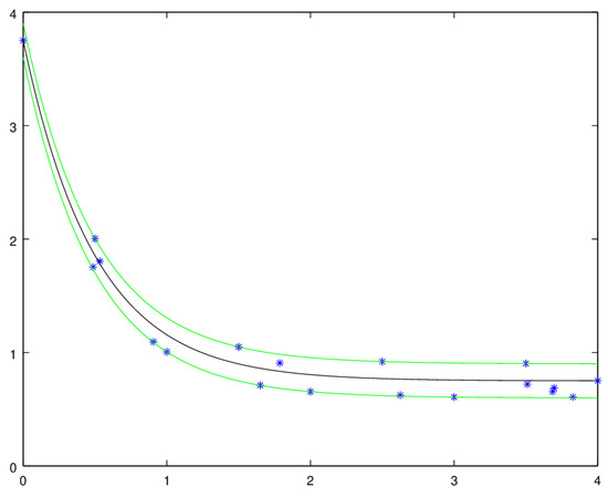
Figure 1.
In blue, the points, in black the best approximation and in green the upper and lower borders of the narrowest band that contains . The band has constant width.
We will need the following definition:
Definition 1.
A real function defined in a linear topological space X is quasiconvex whenever it fulfills
This definition can be consulted in, for example, [1] or [6].
The authors already proved in [1] that for every , there exists the best approximation amongst all the functions of the form , with . We also showed that, given any dataset , the function that assigns to every the error is quasiconvex, so there are two options: either attains its minimum at some k or it is monotonic. If is monotonic, then either it is increasing and the minimum would be attained, so to say, at , or it is decreasing and attains its minimum at . We will also study what happens for positive k, so we will need to pay attention not only to the behaviour of the exponentials but also to their limits when and ; see Proposition 2 and Section 3.2.
Remark 1.
whenever is a different exponential.
Our main results show that every dataset with at least four data fulfills one of the following conditions:
- There exists one triple with such that is the best possible approximation, i.e.,
- There are two indices where is attained and there is some , with , such that . In this case, the best approximation by means of exponentials does not exist and the constant approximates better than any strictly monotonic function—in particular any exponential. Therefore, for every , the best approximation with the form has and . Exactly the same happens when the maximum is attained at and the minimum at and , with . In both cases, the function is constant.
- , and T attains its second greatest value at . The best approximation by means of exponentials does not exist and every exponential approximates worse than any function fulfiling for . The pointwise limit of the best approximations when takes these values. (The symmetric cases belong to these kind of limits, with instead of .) If this happens, increases in
- There are some such that the line approximates better than any exponential. In this case, each is the limit when of the values in of the best approximations with k as exponent. This happens when there are four indices or such that
This implies that decreases in
Remark 2.
What happens with this kind of functions is the following: consider two exponentials that agree at , say . Then, the following are equivalent:
- for some .
- for every .
- for some .
- for every .
A visual way to look at this is the following. Consider a wooden slat supported on two points, and imagine we put a load between the supports. When we increase the load, the slat lowers between the two supports but the other part of the slat raises. For these functions, the behaviour is similar—if two of them agree at α and β, then one function is greater than the other in and lower outside .
Besides, if and then for each that does not lie in the line defined by and and belongs to
there is exactly one exponential h such that , and . Of course, if does not belong to the set given by (1), then there is no monotonic function that fulfils the latter. The existence of such an exponential is a straightforward consequence of [1], Lemma 2.10—we will develop this later, see Proposition 4.
Remark 3.
A significant problem when dealing with the problem of approximating datasets with exponentials has been to find conditions determining whether some dataset is worth trying or not. The only way we have found to answer this problem has been to identify the most general conditions that ensure that some dataset has one best approximation by exponentials—needless to say, this has been a very sinewy problem. The different behaviors described in Remark 1 can give a hint about the several different details that we will need to deal with, but there is still some casuistry that we need to break down. Specifically, our main interest in these results comes from the fact that they can be applied to exponential decays, which appear in several real-life problems—the introduction in [1] presents quite a few examples. The typical data that we have worked with are easily recognizable, but we needed to determine when the data may be fitted with a decreasing, convex function—like the exponentials with . The easiest way we have found is as follows:
- If some data are to be fitted with a decreasing function and we are measuring the error with the max-norm, then the maximum value in T must be attained before the minimum. There may exist more than one index where they are attained, but every appearance of the maximum must lie before every appearance of the minimum. In short, if and , then .
- Moreover, if we are going to approximate with a convex function, the dataset must have some kind of convexity. The only way we have found to state this is as follows:♡ “Let be the line that best approximates . Then has two maxima and one minimum between them.”Thanks to Chebyshev’s Alternation Theorem (the polynomial is the best approximation of function f in if and only if there exists points where attains its maximum and ; see for example [7], Theorem 8, p. 29 or [8]) we know that the line that best approximates any dataset behaves this way, the opposite way or as described in Remark 1. Please observe that this Theorem would not apply so easily to approximations with general degree polynomials.
Before we go any further, let us comment something about the notation that will be used. For the remainder of the paper, we will always take n as the number of coordinates of and T, i.e., . In addition, will fulfil .
Moreover, for any we will always denote as the best approximation with the form with .
To ease the notation, whenever we have some function and , we will let denote , and the same will apply to any fraktur character: would represent the same for and so on.
Given any vector , will denote its maximum and will denote its minimum.
2. Small Datasets
In this Section, we show some not too complicated, general results about the behavior of exponentials that will allow us to prove our main results in Section 4. We will focus only on the approximation of the most simple datasets, with or .
We will begin with Proposition 1, just a slight modification of [1], Proposition 2.3 that will be useful for the subsequent results. Later, in Lemma 1, we will find the expression of the best approximation for for each fixed k (please note that with , for every k there is an exponential that interpolates the data). In Lemma 2, we study the case , determining a technical condition on that ensures that the best approximation exists and it is unique, and moreover, we kind of determine analytically this best approximation.
Proposition 1
([1]). Let , such that is the best approximation to T for this k, i.e.,
Then, there exist indices such that .
Reciprocally, if and fulfil this condition, then is the best approximation to T for this k.
Lemma 1.
Let , and . Then, the best approximation to by means of exponentials has these coefficients:
Proof.
It is clear that , and a simple computation shows that also holds. Indeed,
By Proposition 1, this is enough to ensure that and are optimal. □
Remark 4.
Please observe that does not depend on .
Lemma 2.
Let and such that . Then, there exists a unique exponential , with and such that
Moreover, this exponential is the best approximation to .
Proof.
Let be as in the statement. For , there exist unique such that and . Specifically, a is as in (3) and .
Indeed, means that , so and each determines . The same way, determines .
Therefore, the equalities (4) hold if and only if, for some , we have . Equivalently,
Please observe that this equality holds trivially when and that, as both and are positive, we are not trying to divide by 0.
If we put , the last equality can be written as
We will denote as the left hand side of this equality.
As we are only interested in positive roots of p, we can divide by and consider with for .
Taking into account that , that q obviously vanishes at 1 (but this root corresponds to the void case and so and are not defined) and also that the limit of is ∞ as z goes to ∞, there must exist another , maybe , such that . By Descartes’ rule of signs—see [9], Theorem 2.2—both q and p have at most two positive roots, so there is exactly one other positive root of p. To determine whether this root is greater or smaller than 1, we can compute the derivative of p at 1.
so . This is positive provided , so the other root of p lies between 0 and 1 whenever the condition in the statement is fulfiled.
Therefore, there exists just one for which
Now, taking
and , we have the function we were looking for.
Moreover, suppose that there exist such that approximates at least as well as f. We may suppose that . Now, the conditions for can be rewritten as
By [1], Lemma 2.8, this means that . □
Remark 5.
This Lemma gives a kind of analytic solution to the best approximation problem, with the only obstruction of being able to determine the other root of p. In the next section, we do the same with the symmetric cases and give actual analytic solutions to the same problem when the data are not good to be approximated by exponentials, ironically.
3. Symmetric Cases and Limits
In this section, we focus on those cases that do not match with the problem we have in mind but, nevertheless, have their own interest. First, we approach the symmetric cases such as, for example, exponential growths. Second, we approach the limit cases, that is, the ones whose best approximation is not an exponential but the limit as or of exponentials. They are not what one can expect to find while adjusting data that follow an exponential decay, but we have been able to identify when they occur and deal successfully with them.
3.1. Symmetric Cases
If and f are as in the statement of Lemma 2, then a moment’s reflection is enough to realize that:
- 1.
- The t-symmetric data haveas its best approximation.
- 2.
- The T-symmetric data haveas its best approximation.
- 2.
- The bisymmetric data haveas its best approximation.
These symmetries correspond to the following:
- 1.
- If , then there are still two changes of sign in the coefficients of p, so it has another positive root. The difference here is that both a and k are positive. Please observe that this means that , so f must be increasing and increases faster for greater t.
- 2.
- If , then and .
- 3.
- If , then everything goes undisturbed, but we have , so the second root of p is greater than 1. This implies that and .
3.2. Limit Cases
Even if the conditions are not fulfiled by any symmetric version of the dataset, the computations made in the proof of Lemma 2 give the answer to the approximation problem:
If , then is a double root—this corresponds to —and the “exponential” we are looking for is a line with negative slope. Namely, its slope is and this best approximation is the line given by Chebyshev’s Alternation Theorem.
If , then this “exponential” is a line with positive slope —this is symmetric to the previous case.
If or , then we have, up to symmetries, three cases:
- i:
- If and , then the best approximation is a constant, namely, .
- ii:
- If then there is no global best approximation, but every exponential approximates worse than the limit, with , of the best approximations. This limit isand it turns out to be also a kind of best approximation for every .
- iii:
- If then the situation is as follows:As lies before , any good approximation must be non-increasing. T attains its second greatest value after , so every decreasing function approximates worse than the function defined as in (6). Actually, could be ignored whenever , as we are about to see in the last item.
Finally, if and have different signs, then there is just one change of signs in the coefficients of p, so the only positive root of p is and , and there is no function fulfilling the statement. More precisely, this situation has two paradigmatic examples with and or with and .
In the first case, the third point simply does not affect the approximation in the sense that, for every k, the exponential that best approximates T fulfils
Namely, if is decreasing then , so is neither nor . If is increasing then for , and this, along with Proposition 1, implies that cannot be the best approximation.
The second case is similar. Though the point is relevant for some approximations, it is skippable for every for some .
4. General Datasets
In this Section, we apply the previous results to datasets with arbitrary size in order to find out when a dataset has an exponential as its best approximation. Before we arrive to this first objective’s main result, Theorem 1, we will need several minor results. The path that we will follow is, in a nutshell, the following:
Lemma 3 is a technical Lemma that allows us to show that the maps , , are continuous; see Corollary 1.
Lemma 4 is just Chebyshev’s Alternation Theorem, and it suffices to determine which datasets are good to be approximated by decreasing, convex functions—like exponential decays. We will call these datasets admissible from Definition 2 on.
Then, we determine the vectors one obtains by taking limits of exponentials with exponents converging to or 0; see Proposition 2.
With all these preparations, we are ready to translate Lemma 2 to a more general statement, keeping the condition. We give a necessary and sufficient condition for any dataset to be approximable by exponential decays in terms that are easily generalizable to . This is Proposition 3.
In Proposition 3 and Remark 7, we improve the results in Corollary 1 to get Remark 8, where we show that we can handle the best approximations at ease if the variations of k are small enough.
Finally, Proposition 5 reduces the general problem to the case, thus getting Theorem 1.
Lemma 3.
Let and be the best approximation for and suppose that there are exactly three indices such that the equalities
hold. Then, there exists such that, for every the equalities hold with the same indices. Moreover, if is such that the indices where the norm is attained are not , then there exists for which the norm is attained in at least four indices.
Proof.
Suppose , the case is symmetric.
As —see Lemma 1—taking for every we have . If we take, further
then , so defining we get and a straightforward computation shows that
for every k. Given any , our hypotheses give
As the map is continuous for every l, we obtain that
holds for every k in a neighbourhood of , say . Since there are only finitely many indices, we may take as the minimum of the to see that is the best approximation for , and finish the proof of the first part.
Moreover, it is quite obvious that the expression for will be with
if and only if, for every , one has
Please observe that the symmetric inequalities could hold and it would make have the same expression, but this would imply . In any case, if is such that there is some l for which
then it is clear that there is such that
Maybe it is not , but taking as the smallest real number in for which there exists such an l, we are done. □
Corollary 1.
The maps and are continuous.
Lemma 4.
Let . There exists exactly one line such that
for some and , and this line approximates T better than any other line.
Proof.
It is a particular case of the Chebyshev’s Alternation Theorem, applied to the polygonal defined by . □
Remark 6.
Thanks to Lemma 4, we can define which vectors T will be our “good vectors”: those for which and the equalities (8) hold with and not with . When data fulfil these conditions, we have some idea of decreasing monotonicity and also some kind of convexity, and this is the kind of dataset that we wanted, though we will need to add some further conditions. Anyway, when dealing with datasets that fulfil any couple of symmetric conditions, we just need to have in mind the symmetries. Specifically, they will behave as in Section 3.1.
Definition 2.
Let be the line that best approximates . We will say that is admissible when and there exist such that
- 1.
- 2.
- for every and every .
- 3.
- for every .
Once we have stated the kind of data which we will focus on, say discretely decreasing and convex, now we have to determine when they will be approximable. Before that, we will study the behavior of the limits of best approximations.
Lemma 5.
Let . For each , consider some exponential and
Then depends on k but not on or , and moreover:
- 1.
- When
- 2.
- When ,
- 3.
- When .
Proof.
We only need to make some elementary computations to show that
The computation of the limit at 0 only needs a L’Hôpital’s rule application, and the other ones are even easier once one substitutes . See [1] (lemma 2.10). □
Proposition 2.
Let . Then, the following hold:
- 1.
- For , .
- 2.
- For , is , the line that best approximates .
- 3.
- For , takes at most two values, and fulfils
- 4.
- For , takes at most two values, and fulfils
Proof.
Let . If the best approximation for is a constant, then it is constant for every , and the constants are obviously the same. Therefore, we may suppose is not a constant for any . In this case, Lemma 3 implies that is continuous for every l. As we have just a finite amount of indices, this means that so we are done.
The proof of the three last items is immediate from Lemma 5. □
Proposition 3.
Let and . Then, the best exponential approximation to has the form with if and only if is admissible and the following does not happen:
and the second greatest value of T is attained after .
Proof.
As the second greatest value of T will appear frequently in this proof, we will denote it as . Analogously,
If ♠ happens, then the following expression is the limit of best approximations when
Indeed, as is the pointwise limit of functions fulfiling (2), it must fulfil (2) as well. It is clear that this implies that must be as in (9). It is clear that every strictly decreasing function approximates worse than , so we have finished the first part of the proof.
Conversely, if is admissible, then there are exponentials with that approximate better than the line . Indeed, we only have to consider the three points of the Definition 2 and take into account Lemma 3. As the function error is quasiconvex, the only option for contradicting the statement is that every exponential is worse than the limit of the approximations , and of course this limit is not better than as in (9) because no vector of the form approximates T better than this. Therefore, we may suppose is the best approximation—recall that we are supposing that is admissible. We need to break down several possibilities:
- I:
- If , then we can change the first coordinate of from to without increasing the error, so one best approximation is a constant, and this means that , so is not admissible, a contradiction.
- II:
- If , then is not admissible.
- III:
- If , then we still have some options:
- i:
- If then we obtain that ♠ holds, no matter the value of .
- ii:
- If and the rate of decreasing is greater than , then fulfils the hypotheses of Lemma 2. This implies that the best approximation to has , so the best approximation to has .
- iii:
- If and the rates of decreasing are equal, then is not admissible because this implies
- iv:
- If and , then Lemma 2 ensures that the best approximation is , with and . □
Remark 7.
Let be the line that contains and . In [1] (lemma 2.10), it is seen that, if , where
then and
- As , .
- As , .
- As , .
Essentially, the same proof suffices to show how behaves:
- As , .
- As , .
- As , .
This implies that the map is strictly increasing, while is strictly decreasing. So, increases as decreases, and, moreover, the map given by for and is a (decreasing) homeomorphism from to . Applying the same reasoning to and to , we obtain this key result:
Proposition 4.
Let and and consider for every the only exponential such that and the only line such that . Then, all the following maps are homeomorphisms, and are decreasing and is increasing:
- 1.
- defined as .
- 2.
- defined as .
- 3.
- defined as .
We can rewrite Proposition 4 as follows:
Remark 8.
Let and . Let, for every , be the only exponential that fulfils . Then, when k increases, and decrease and increases and everything is continuous.
Proposition 5.
The best exponential approximation (including limits) to is the best approximation for some quartet
Proof.
Let be the best approximation, and suppose that the conclusion does not hold. Then, we may suppose that there are exactly three indices where the norm is attained, say and
If is the limit at of the best approximations, then it is the best approximation for every quartet that contains because this means that ♠ holds. Therefore, suppose that the best approximation is , for some – maybe . Then, for some the functions , with approximate this triple better than . Reducing if necessary , Remark 8 implies that every with approximates better than , thus getting a contradiction. □
Theorem 1.
Let be admissible. Then, the best approximation is a exponential if and only if ♠ does not happen.
Proof.
The proof of Proposition 3 is enough to see that ♠ avoids the option of being approximable by a best exponential.
If is admissible, then the best approximation cannot be the 0-limit of exponentials, so it is either an exponential or the -limit of exponentials. So, suppose it is the -limit and let us see that in this case ♠ holds. It is clear that as in the proof of Proposition 3, so just need to show that occurs later than . Let . A moment’s reflection suffices to realize that for every , so the error for is exactly . Let be the last appearance of and the first appearance of , and suppose , i.e., that ♠ does not hold. Thanks to Proposition 4, for small , there is k close enough to that we can find such that , when and when . If we take small enough, approximates better than . □
The value of b in (3) can be easily generalised, so we do not need to worry about it. If we are able to determine k and , then finding b is just a straightforward computation. Namely, the following Lemma solves it:
Lemma 6.
For , the best approximation to T in is attained when
With this b, the error is
Proof.
On the one hand, this implies that the error is as in the statement. On the other hand, let . Then,
so approximates T worse than . The same happens with if we take , so the best approximation is the one with b as in (10). □
With this section, we have covered the theoretical aspects about the first objective of this paper. Examples in Section 5 are about Newton Law of Cooling and directly apply what have been developed here, ending this way the first objective.
5. Examples
In this section, we present two different examples. We intend to apply what has been developed in previous sections to fit exponential functions to some data.
The calculations in this section were carried out by means of a GNU Octave using an AMD Ryzen 7 3700U processor with 16 GB of RAM. The system used is an elementary OS 5.1.7 Hera (64-bit) based on Ubuntu 18.04.4 LTS with a Linux kernel 5.4.0-65-generic.
5.1. Exponential Decay in a Newton’s Law of Cooling Process
In [1], Section 4, the paper that motivated this one, we presented an example that was the beginning of our work. In this new approach we consider necessary to fit the same pattern with the same data but using a new tool: approximation through the max-norm.
We are going to use data coming from a thermometer achieving thermal balance at the bottom of the ocean. The time evolution of the temperature, according to Newton’s law of cooling process, follows an exponential function as
where and and, in the considered case, .
We implemented an algorithm to fit, by a pattern as (11), and taking the max-norm as the approximation criteria, the records obtained by the device. The results corresponding to this implementation are gathered in Table 1. Table 2 of [1] shows similar information for the same fit but using the Euclidean norm, so interested readers can compare both approximations.

Table 1.
Result of implementation of TAC (Spanish for CT scan).
In Figure 2, we present some graphical information about this approximation. Figure 2a shows observations and fit, and Figure 2b shows the relative error in this implementation. We have designed this figures to resemble [1], Figure 3 so the reader can graphically compare the results of both approximations. Taking into account that each example uses a different norm, differences in the fit must exist. Nevertheless, they both give a more than reasonable approximation.
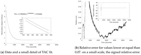
Figure 2.
Some graphical aspects of this TAC implementation. In the numerical analysis bibliography, relative error is defined with or without sign; in this paper, we will consider the latter. A spike can be seen in the small window of (b). This spike should not be considered as an indicator of a poor adjustment of the curve to the data. On the contrary: the spike is due to the proximity of the data to zero; however, the error remains bounded. This is because curve and data are close enough to control the fact that we are virtually dividing by zero.
5.2. Exponential Decay Attaining the Max-Norm in 4 Indices
We wanted to include an example to illustrate the meaning of Proposition 5. The data considered in Section 5.1 were difficult to approach with the implementation we have wrote for max-norm, which is in a very early stage. We have been able to approximate a dataset of the same nature but maybe with a more adequate distribution. For this implementation, we present in Figure 3 the four points prescribed by Proposition 5 coloured in red.
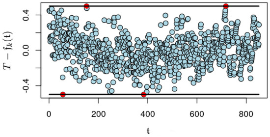
Figure 3.
Blue dots represent differences between T and . In 4 dots, and are reached, and we have colored them in red. Those are the 4 points mentioned in Proposition 5. Please observe how the maxima and the minima are alternatively reached.
6. Economical Models and nlstac
Now we will cover the second objective: to exemplify the interest for the economic science of the algorithm presented in [1] and implemented in the R-package nlstac. The calculations in this section were carried out by the same machine as in Section 5 using RStudio instead of GNU Octave.
6.1. The Exponential Model in Demand Curves
In this example, we will use the exponential model to fit demand curves. As stated in [10], “behavioral economic demand analyses describe the relationship between the price (including monetary cost and/or effort) of a commodity and the amount of that commodity that is consumed. Such analyses have been successful in quantifying the reinforcing efficacy of commodities including drugs of abuse, and have been shown to be related to other markers of addiction”.
Different mathematical representations of demand curves have been proposed—see, for example, [3]. The most widely used model for demand curves in addiction research is presented in the following equation
where Q represents consumption at a given price, is known as derived demand intensity, k is a constant that denotes the range of consumption values in log units, C is the commodity price and is the derived essential value, a measure of demand elasticity.
This model was established by Hursh and Silberberg in [3] and has been used in many other works such as [10,11,12]. The parameters to be estimated are , k and .
Renaming as b, k as a and as d, the pattern is now similar to the one we have been working in this paper:
Therefore we simply need to adjust the pattern presented in (13) to consumption data and undo the changes, with , and being the parameters we originally sought.
We ran a simulation for this kind of data and successfully fitted the pattern using R package nlstac. For the simulation, we have established 15 as the number of observations, as 48, as 0.006 and k as 3.42 and added some noise to the pattern with mean 0 and standard deviation . Tolerance value was set as 10.
Table 2 shows the result of this TAC implementation. As can be seen, output is reasonably similar to the values we originally established. Please take into account that we added some noise to the data so differences in the parameters were expected.
Table 2.
Result of implementation of nlstac for pattern (12). RSS denotes residual sum of squares, and where is the number of observations.
In Figure 4, we can see the observations (blue dots) and the approximation (red dots). This approximation makes sense: it is in the middle of the observations, keeping the errors under control.
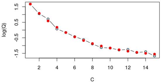
Figure 4.
Observations in blue, approximation in red.
6.2. The Exponential Autoregressive Model
As stated in [13], “nonlinear time series models can reveal nonlinear features of many practical processes, and they are widely used in finance, ecology and some other fields”. Out of those nonlinear time series models, the exponential autoregressive (ExpAR) model is especially relevant. Given a time series , the ExpAR model is defined as
where are independent and identically distributed random variables and independent with , p denotes the system degree, , , and , (for ) and are the parameters to be estimated from observations. This model can be found in, for example, [13] or [14]. We have followed the notation of the former.
Some generalizations for this model have been made, and [14] presents a wide variety of those generalizations. Teräsvirta’s model is an extension of the ExpAR model presented in [15] and used in [14]. We will focus on a generalization of Teräsvirta’s model that can be found in [14], Equation (10):
where (for ) are scalar parameters and d is an integer number.
We intend to fit (14) in the particular case when for some data. Please observe that this problem is way beyond the proven convergence of TAC algorithm. It requires more than just fitting of a curve following some exponential function since now we have no function to be fitted because every observation depends on the previous ones. This obstacle can be overcome by looking at the problem not as a one-dimensional problem but as a two-dimensional one: if are the observations, denoting , , , , and , data y will depend on two independent variables, and , and could be written as
where operator ζ represents the element-wise product of two vectors, that is, given , , and where the exponential and power functions are applied coordinate-wise.
As indicated before, this new approach is far from proven in the TAC convergence; however, running nlstac package will provide us a result that stands to reason.
For the simulation, we have considered in (14) . We have generated the 100 first elements of the time series setting as −1.49, as , as , as −0.44, as −0.84, as , as , as , as , as , and tolerance as .
In Table 3 and Table 4, we gather the results of this implementation. As can be seen, parameters are quite similar to the ones we have previously established.
Table 3.
Result of implementation of nlstac for pattern (14).
Table 4.
Result of implementation of nlstac for pattern (14), with RSS being residual sum of squares and where is the number of observations.
In Figure 5, we can see the approximations (red dots) over the actual observations (blue dots, a bit bigger than the red ones), which indicate that the approximation is good.
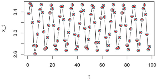
Figure 5.
Observations in blue, approximation in red (smaller circle). Please observe how each approximation lays over the actual observation.
This example is especially relevant because it shows us the possibility to use nlstac in a problem significantly different from the one it was intended for, so it opens the door to its use in different nonlinear time series models or even in some other models.
6.3. The Exponential Autoregressive Model. Applications to Real Data
In order to get a broader perspective about the utility of TAC in relation to the ExpAR model, we have included in this subsection an application of the ExpAR model to real data. The ExpAR model and several generalization has been used in [5] as the fitting model for real data from S&P500 and several other indices.
For this application we have used the S&P500 index, which is a stock market index that measures the stock performance of 500 large companies listed on stock exchanges in the United States. It is often thought to be a good representation of the United States stock market.
We have considered the first differences of the daily close values on S&P500 from 1 January 2000 until 31 December 2020 as the data. These data are public and can be consulted in https://finance.yahoo.com ( accessed on 31 March 2021).
We will present a couple of examples where the same data are processed through two different generalizations of the ExpAR model. In both implementations we fit the models by TAC.
For the first implementation, we have used the first-order Extended ExpAR model defined in [5], taking an order 4 polynomial:
As stated in [5], when the order of the polynomial is greater than 2, the model becomes very complicated, and it is usually avoided because of its complexity. In our case, the complexity of the calculations remain virtually the same since increasing the order of the polynomial just increases the number of linear parameters, which are easily computed, but not the number of nonlinear ones.
Table 5.
Result of implementation of nlstac for pattern (16) taking a tolerance of , the number of divisions as 50 and as the interval where to seek the nonlinear parameter .
Table 6.
Result of implementation of nlstac for pattern (16), RSS being the residual sum of squares and where n = 5282 is the number of observations.
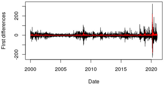
Figure 6.
First differences in black, approximation in red. Implementation using pattern (16).
Once we have established that the order of the polynomial does not make the fit any more complex, let us choose a different model with different nonlinear parameters and different lags. We have chosen the following model:
Now we have two nonlinear parameters, and , and the problem, as can be seen, is quite a bit more complex than the previous implementation.
Table 7.
Result of implementation of nlstac for pattern (17) taking a tolerance of , the number of divisions as 10 and and as the intervals where to seek, respectively, the nonlinear parameters and .
Table 8.
Result of implementation of nlstac for pattern (17), RSS being residual sum of squares and where n = 5281 is the number of observations.

Figure 7.
First differences in black, approximation in red. Implementation using pattern (17).
Again, this example shows the possibility to use nlstac in problems that are different from the ones that it was initially designed for.
7. Conclusions
Thoughout the present paper, we have been able to determine the exact conditions that some dataset need to have a best-fitting exponential function, we have found conditions that the coefficients of this exponential must fulfil if there is such a function and we have been able to show how to approximate these coefficients with the R-package nlstac.
Moreover, we have applied nlstac in a straightforward manner to a pattern provided by an economic model. Furthermore, we have challenged our method, approximating with it very different patterns given by some generalizations of the ExpAR model. Implementations use both simulated and real data. All implementations converge with reasonable computer and time of processing requirements (the hardest, 27.574 s). In all these implementations, we checked the utility of nlstac for fitting complex patterns and also checked the goodness of those fits.
Author Contributions
As can be deduced by the acknowledgments, all authors have been involved during the whole creative process of this paper. However, we would like to note that the contributions of J.C.S. have been crucial in the results involving the max-norm. This same comment can be suitable for the examples presented in this paper, where J.A.F.T. has had a predominant role. Nevertheless M.R.A. was key to obtaining the final version of the paper, connecting both major goals of this paper. All authors have read and agreed to the published version of the manuscript.
Funding
This research was partially supported by MICINN [research project references CTM2010-09635 (subprogramme ANT) and PID2019-103961GB-C21], MINECO [research project reference MTM2016-76958-C2-1-P], European Regional Development Fund and Consejería de Economía e Infraestructuras de la Junta de Extremadura [research projects references: GR18097, IB16056 and GR15152].
Institutional Review Board Statement
Not applicable.
Informed Consent Statement
Not applicable.
Data Availability Statement
Not available.
Acknowledgments
We thank our workmates, who always had interesting comments or hints during coffee breaks. Each author is grateful to the rest for their good attitude, which promoted a positive working atmosphere. The endurance of Javier Cabello Sánchez has been key in this work, and the other authors are grateful to him.
Conflicts of Interest
The authors declare no conflict of interest.
Abbreviations
The following abbreviations are used in this manuscript:
| ExpAR | Exponential autoregressive model |
| TAC | Spanish for CT scan |
| S&P500 | Standard & Poor’s 500 |
References
- Fernández Torvisco, J.A.; Rodríguez-Arias Fernández, M.; Cabello Sánchez, J. A new algorithm to fit exponential decays. Filomat 2018, 32, 4233–4248. [Google Scholar] [CrossRef]
- Rodríguez-Arias, M.; Fernández, J.A.; Cabello, J.; Benítez, R. R Package nlstac. Version 0.1.0. 2020. Available online: https://CRAN.R-project.org/package=nlstac (accessed on 31 March 2021).
- Hursh, S.; Silberberg, A. Economic Demand and Essential Value. Psychol. Rev. 2008, 115, 186–198. [Google Scholar] [CrossRef] [PubMed]
- Franses, P.H.; Dijk, D.V. Non-Linear Time Series Models in Empirical Finance; Cambridge University Press: Cambridge, UK, 2000. [Google Scholar] [CrossRef]
- Katsiampa, P. Nonlinear Exponential Autoregressive Time Series Models with Conditional Heteroskedastic Errors with Applications to Economics and Finance. Ph.D. Thesis, Loughborough University, Loughborough, UK, 2015. [Google Scholar]
- Greenberg, H.J.; Pierskalla, W.P. A Review of Quasi-Convex Functions. Oper. Res. 1971, 19, 1553–1570. [Google Scholar] [CrossRef]
- Lorentz, G. Approximation of Functions; Chelsea Pub. Co: New York, NY, USA, 1986; ISBN 0828403228. [Google Scholar]
- Poreda, S. Complex Chebyshev alterations. Pac. J. Math. 1972, 40, 197–199. [Google Scholar] [CrossRef][Green Version]
- Haukkanen, P.; Tossavainen, T. A generalization of Descartes’ rule of signs and fundamental theorem of algebra. Appl. Math. Comput. 2011, 218, 1203–1207. [Google Scholar] [CrossRef]
- Koffarnus, M.; Franck, C.; Stein, J.; Bickel, W. A Modified Exponential Behavioral Economic Demand Model to Better Describe Consumption Data. Exp. Clin. Psychopharmacol. 2015, 23. [Google Scholar] [CrossRef] [PubMed]
- Christensen, C.; Silberberg, A.; Hursh, S.; Roma, P.; Riley, A. Demand for Cocaine and Food over Time. Pharmacol. Biochem. Behav. 2008, 91, 209–216. [Google Scholar] [CrossRef] [PubMed][Green Version]
- Strickland, J.; Lile, J.; Rush, C.; Stoops, W. Comparing exponential and exponentiated models of drug demand in cocaine users. Exp. Clin. Psychopharmacol. 2016, 24, 447–455. [Google Scholar] [CrossRef] [PubMed]
- Xu, H.; Ding, F.; Yang, E. Modeling a nonlinear process using the exponential autoregressive time series model. Nonlinear Dyn. 2019, 95. [Google Scholar] [CrossRef]
- Chen, G.Y.; Gan, M.; Chen, G.L. Generalized Exponential Autoregressive Models for Nonlinear Time Series: Stationarity, Estimation and Applications. Inf. Sci. 2018, 438. [Google Scholar] [CrossRef]
- Teräsvirta, T. Specification, Estimation, and Evaluation of Smooth Transition Autoregressive Models. J. Am. Stat. Assoc. 1994, 89, 208–218. [Google Scholar] [CrossRef]
Publisher’s Note: MDPI stays neutral with regard to jurisdictional claims in published maps and institutional affiliations. |
© 2021 by the authors. Licensee MDPI, Basel, Switzerland. This article is an open access article distributed under the terms and conditions of the Creative Commons Attribution (CC BY) license (https://creativecommons.org/licenses/by/4.0/).