Abstract
In this paper, we introduce a robust version of the empirical likelihood estimator for semiparametric moment condition models. This estimator is obtained by minimizing the modified Kullback–Leibler divergence, in its dual form, using truncated orthogonality functions. We prove the robustness and the consistency of the new estimator. The performance of the robust empirical likelihood estimator is illustrated through examples based on Monte Carlo simulations.
1. Introduction
A moment condition model is a family of probability measures (p.m.), all defined on the same measurable space , such that (s.t.)
where is the Borel -field. The parameter of interest belongs to a compact set and the function , with , is defined on , each component being real valued function. Denote by the set of all probability measures on , and for each define
so that
Let be an i.i.d. sample with unknown p.m. . We assume that the equation has a unique solution (in ), which will be denoted . We consider the estimation problem of from the data . The traditional way of estimating the parameter is given by the Generalized Method of Moments (GMM) [1]. The GMM estimators are consistent and have asymptotically normal distribution. Despite their desirable asymptotic properties, the finite sample performance of the GMM estimators is not satisfactory. Some other alternative methods have been proposed in the literature. The Continuous Updating (CU) estimator [2], the Empirical Likelihood (EL) estimator [3,4,5], and the Exponential Tilting (ET) [6], are three of the most known examples. Imbens [7] showed that EL and ET estimators are characterized by lower bias than GMM in nonlinear models. Newey and Smith [8] studied the theoretical properties of EL, ET, and CU estimators, by including them into the Generalized Empirical Likelihood (GEL) family of estimators, and showed that all GEL estimators are characterized by lower asymptotic bias than GMM. The information and entropy econometric (IEE) techniques have been proposed in order to improve the finite sample performance of the GMM estimators and tests [4,6]. Ronchetti and Trojani [9] and Lo and Ronchetti [10] have proposed robust alternatives for GMM estimators and tests, respectively, for the IEE techniques, keeping also the finite sample accuracy. Felipe et al. [11] proposed empirical divergence test statistics based on exponentially tilted empirical likelihood estimator with good robustness properties. Broniatowski and Keziou [12] proposed a general approach for estimation and testing in moment condition models, which includes some of the above-mentioned methods. This approach, based on minimizing divergences with their dual forms, allows the asymptotic study of the estimators (called minimum empirical divergence estimators) and of the associated test statistics, both under the model and under mis-specification of the model. The approach based on divergences and duality was firstly considered in the case of parametric models, for example, in [13,14,15]. Applications of the minimum dual divergence estimators in model selection problems are considered in [16].
The EL paradigm enters as a special case of the general methodology from Broniatowski and Keziou [12], namely, when using the modified Kullback–Leibler divergence. Although the EL estimator is preferable to other estimators due to higher-order asymptotic properties, these properties are valid only in the case of the correct specification of the moment conditions. On the other hand, when the support of the p.m. corresponding to the model and the orthogonality functions are not bounded, the EL estimator may cease to be root n consistent (Schennach [17]) under mis-specification. It is a known fact that the EL estimator for moment condition models is not robust. This fact is also justified by the results from [18], where it is shown that the influence function of a minimum dual divergence estimator, and particularly that of the EL estimator, is linear related to the orthogonality function g corresponding to the model. Thus, the influence function of the EL estimator is bounded if and only if the function g corresponding to the underlying model is bounded. Hence, the EL estimator is usually not robust, since the function g could be unbounded on the observation. For this reason, in practice, the classical EL estimator, as well as the minimum dual divergence estimators and also GMM estimators, is unstable even under small deviations from the assumed model.
As examples in this context, we mention models for which the orthogonality functions are unbounded [9]. The autoregressive models with heteroscedastic errors [19] can be written under the form of moment condition models, but the orthogonality functions defining the orthogonality conditions are unbounded. Moreover, the nonlinear empirical asset pricing models [20] can be written under the form of moment condition models and have natural orthogonality conditions (given by the given asset pricing equations), which are given by unbounded orthogonality functions. We also recall the following classical example, which is used in the last section of the paper, in the Monte Carlo simulation study.
Example 1
([3] p. 302). Consider a random variable X with unbounded support ( or for instance). Let , and assume that , with being a known function. The aim is to estimate the parameter θ using an i.i.d. sample of X. The information on the probability distribution of X can be expressed in the context of model (1), with and , by taking . One can see that the orthogonality functions and are unbounded (with respect to x).
For such models, the lack of robustness of the EL estimator, as well as the lack of robustness of other classical estimators, represents the motivation to study some robust alternatives.
In the present paper, we propose a locally robust version of the EL estimator for moment condition models. Locally robust in the sense that the functional associated with this estimator is locally approximated by the means of the influence function, and then, the boundedness of the influence function will imply the fact that, in the neighborhood of the model, the asymptotic bias of the estimator cannot become arbitrarily large (see [21]). The new estimator is defined by minimization of an empirical version of the modified Kullback–Leibler divergence in dual form, using truncated orthogonality functions. This leads to a robust EL estimate. Moreover, we prove the consistency of this estimator, Finally, we present an example based on Monte Carlo simulations illustrating the performance of the robust EL estimator in the case of contaminated data.
2. A Robust Version of the Empirical Likelihood Estimator
2.1. Statistical Divergences
Let be a convex function on onto valued, satisfying . Let P be some p.m. on the measurable space . For any signed finite measure Q, on the same measurable space , absolutely continuous with respect to P, the -divergence (sometimes we simply say divergence) between Q and P is defined by
where is the Radon–Nikodym derivative. When Q is not absolutely continuous with respect to we set . This definition extends the one given in [22] for divergences between p.m.’s. A known class of divergences between p.m.’s is the class of Cressie–Read divergences, introduced in [23] and defined by the functions
for , and . For any , if is not defined, we set , which may be finite or infinite. The Kullback–Leibler divergence () is associated to , the modified Kullback–Leibler () to , the divergence to , the modified divergence () to and the Hellinger (H) distance to . The -divergence between some set of probability measures and a probability measure P is defined by
2.2. Definition of the Estimator
We consider a reference identifiable model of probability measures such that, for each , , which means that , and assume that is the unique solution of the equation. We assume that the p.m. of the data corresponding to the true unknown value of the parameter to be estimated belongs to this reference model. The reference model will be associated with the truncated orthogonality function that will be used to define the robust version of the EL estimator of the parameter . We will use the notation for the Euclidean norm. Similarly as in [9], using the reference model , we define the function ,
where is the Huber’s function
and , are, respectively, -matrix and ℓ-vector, defined as the solutions of the system of implicit equations
where is the identity matrix and is a given positive constant. Therefore, we have , for all x and . We also use the function
when needed to work with the dependence on the matrix A and on the vector . Therefore,
For given from the reference model, the triplet is the unique solution of the system
see [9], p. 48.
Consider the estimating problem of the triplet on the basis of a sample , . For each , using the p.m. from the reference model, we define and , solutions of the system
where is the empirical measure associated with the sample,
with being the Dirac measure at the point x, for any x. We denote
Note that depends on both the data and the reference probability . We now consider the moment condition model associated to the function , namely,
where
The p.m. belongs to .
In what follows, we consider the modified Kullback–Leibler divergence, which corresponds to the strictly convex function , if , respectively , if . The convex conjugate, called also the Fenchel–Legendre transform, of any function , is the function defined by , for all . A straightforward calculus shows that the convex conjugate of the convex function , denote it , is given by if , respectively , if . For given , we define the set
where . We denote and
Since is bounded (with respect to x), on the basis of Theorem 1.1 in [24] and Proposition 4.2 in [12], the following dual representation of -divergence holds
where
and the supremum in (16) is reached, provided that is finite. Note that depends on the reference p.m. , since depends on . W denote then any vector such that
Furthermore, according to Proposition 4.2 from [12], for each , the condition
ensures that , defined as solution of optimization problem (18), is unique. Notice that the linear independence of the functions implies condition (19) whenever is not degenerate.
Moreover, using again Proposition 4.2 and Remark 4.4 from [12], for each , one can show that the first component of the optimal solution in (18) equals to zero. One can then omit the first component of the vector in displays ((15)–(18)). Therefore, they will be replaced by
where
and
Denote
In view of relation (23), a natural estimator of , is defined by
Then, a “dual” plug-in estimator of the modified Kullback–Leibler divergence, between and , can be defined by
where is the extended logarithm function, i.e., the function defined by if , and if , for any Finally, we define the following estimator of
which can be seen as a “robust” version of the well-known EL estimator.
Recall that the EL estimator can be written as (see, e.g., [5])
For establishing asymptotic properties of the proposed estimators, we need the following additional notations. Consider the moment condition model associated with the truncated function
where and are the solution to the system (7). Note that depends only on the reference model and not on the data. This model is defined by
where
Let
Therefore, as above, we have the following dual representation for
where
and the supremum in (31) is reached, provided that is finite. Moreover, the supremum in (31) is unique under the following assumption
which is satisfied if the functions are linearly independent and is not degenerate. We denote then
Finally, we have
We also use the function
when needed to work with the dependence on matrix A and on vector . We have, then, with the above notation, where and are the solution of the system of Equation (7).
2.3. Robustness Property
In order to prove the robustness of the estimator , we use the following well-known tools from the theory of robust statistics; see, e.g., [21]. A functional T, defined on a set of probability measures and parameter space valued, is called a statistical functional associated with an estimator of the parameter from the model , if . The influence function of T at is defined by
where . A natural robustness requirement on the statistical functional corresponding to the estimator is the boundedness of its influence function.
, with and solutions of the system
and
Note that, for a given , the function , as well as , both depend on the p.m. . In addition, note that coincides with defined in the preceding section. We denote
Then
Proposition 1.
The influence function of the estimator is given by
Proof.
Using the definitions of and , we have
Using (46), since
is solution of the equation
Since the first integral in the above display is 0, according to (44), the above equation simplifies to
By replacing P with the contaminated model in Equation (49) and then derivating with respect to , the resulting equation, we obtain
On the other hand,
Differentiating with respect to of (44) leads to
Some simple calculations yield
and
Then, we obtain
and
By replacing in (53), we obtain
By differentiation with respect to , and taking , we get
Consequently,
By combining (58) with (60), we obtain (43). □
Remark 1.
The classical empirical likelihood estimator of the parameter of the moment condition model can be obtained as a particular case of the class of minimum empirical divergence estimators introduced by Broniatowski and Keziou [12]. Toma [18] proved that, in the case when belongs to the model , the influence functions for the estimators from this class, so particularly the influence function of the EL estimator, are all of the form
irrespective of the used divergence. This influence function also coincides with the influence function of the GMM estimator obtained by Ronchetti and Trojani [9] and is linearly related to the function of the model. When the orthogonality function is not bounded in x, the minimum empirical divergence estimators, and particularly the EL estimator of , are not robust. For many moment condition models, the orthogonality functions are linear and hence unbounded; therefore, these estimation methods are generally not robust. This is also the case of other known estimators, such as the least squares estimators, the GMM estimators, and the exponential tilting estimator for moment condition models. Instead, for the new estimator defined in the present paper, the influence function is linearly related to the function , which is bounded; therefore, this estimator can be seen as a robust version of the classical EL estimator.
An important feature of the robust version of the EL estimator is that its robustness can be controlled by a positive constant c. This constant appears in the Huber function used. In addition, an advantage of this approach based on using the Huber function is that we can require the bound of influence function of the estimator to be satisfied in a norm that is self-standardized with respect to the covariance matrix of the estimator; this norm measures the influence of the estimator relative to its variability expressed by its covariance matrix. Such an approach is also suitable to induce stable testing procedures (see [9]), which could be useful in future studies regarding robust testing. The robust estimator proposed in the present paper has the self-standardized influence function bounded by the constant c appearing in the Huber function. In a similar manner as in [9], the constant c controls the degree of robustness of the estimator, and in practice, we could take a value close to the lower bound in order to enforce a maximum amount of robustness. On the other hand, the density power divergences [25] combined with the minimum divergence approach have proved useful for construction of robust estimators in different contexts, in particular for parameter density estimation. Other approaches for robust estimation in regression models is proposed by [26]. Such approaches could be considered in future research studies in order to be adapted to the context of the moment condition models.
2.4. Consistency of the Estimators
In this subsection, we establish consistency of the estimator of , for any fixed , and the consistency of the estimator of . First, for any fixed , we state the consistency of the estimators and defined by the system (11).
2.4.1. Consistency of the Estimators and , for Fixed
The estimators and , of and defined by the theoretical system of Equation (7), are Z-estimators. We consider the following notations
and , where “” is the operator that transforms the matrix into vector, by putting all the columns of the matrix one under the other. Notice that, is a constant function with respect to x. With these notations, for a given , the Z-estimators and are solutions of the system (see (11)),
and their theoretical counterparts are and solution of the system (see (7)),
In the rest of the paper, we consider matrix A in its “vec” form, as defined above. This is necessary in order to apply some classical results, for example the uniform weak law of large numbers (UWLLN) or results regarding Z-estimators. Therefore, the argument A of the functions , and will be in fact . For simplicity, we write A instead of . The same is valid for and .
Assumption 1.
(a) There exists compact neighborhood of such that
(b) for any positive ε, the following condition holds
where .
Proposition 2.
For each , under Assumption 1, converges in probability to .
Proof.
Since is continuous, by the UWLLN, Assumption 1(a) implies
in probability. This result, together with Assumption 1(b) ensure the convergence in probability of the estimators and toward and , respectively. The arguments are the same as those from [27], Theorem 5.9, p. 46. □
2.4.2. Consistency of the Estimator of , for Fixed
We state the consistency of the estimators under the following assumptions.
Assumption 2.
(a) exists, unique and interior point of ;
(b) there exists a compact neighborhood of such that , and there exists compact neighborhood of such that
(c) there exists compact neighborhood of , and there exists a sequence , such that, for all , it holds
Proposition 3.
Under Assumptions 1 and 2, we have
converges in probability to ;
converges in probability to .
Proof.
(1) Using Assumption 2(b) and the continuity of the function with respect to , and , by the uniform weak law of large numbers (UWLLN), we get
in probability. The following inequality holds
The first term in the right hand side of the Inequality (70), tends to 0 in probability, on the basis of the result (69). The second term in the right hand side of (70) also tends to 0 in probability. Indeed, using the convergence in probability , by Assumption 2(b), we get the pointwise convergence for each t. Then, according to Corollary 2.1 from [28], using the point-wise convergence together with Assumption 2(c), we obtain the uniform convergence
Consequently
in probability. Using (72) and the fact that is unique and belongs to and the strict concavity of the function , on the basis of Theorem 5.7 in [27], we conclude that any value
converges in probability to . We show that belongs to with probability one as , and consequently it converges to . Since for n sufficiently large any , the concavity of the criterion function ensures that no other point t in the complement of can maximize over ; hence belongs to .
(2) We have
Note that
Both the right hand side and the left hand side in the above display tend to 0 in probability using (72). Hence, converges to , in probability. □
2.4.3. Consistency of the Estimator
Assumption 3. the function is continuous, with probability 1;
for each , there exist compact neighborhood of and compact neighborhood of such that
Let . There exists a sequence such that, for all , it holds
the function is continuous on Θ;
exists, unique and interior point of Θ.
Proposition 4.
Under Assumptions 1–3, we have
in probability, uniformly with respect to ;
in probability.
Proof.
(1) By Assumption 3(a), is continuous in . Using also Assumption 3(b), by applying UWLLN, we obtain the uniform convergence in probability
over the compact set We will prove the uniform convergence in probability
Let . We show that for any
We show that belongs to with probability one, as
Let be such that . Since is compact, by continuity, there exists , such that Hence, there exists such that
Therefore,
Using (76), (79), and (80), we deduce that in probability. In particular, for large n, uniformly in . Since is concave, the maximizer belongs to for sufficiently large n. Then, in probability. (2) For large n, we can write
Note that
In order to prove that in probability, we first prove that
in probability. Notice that
The first term in the right-hand side of the above inequality tends to 0 in probability, using (76). Regarding the second term, we have the convergence (71), and combining this with Assumption 3(c), we obtain
in probability. Consequently, (83) holds. Then, (81) and (82) lead to
Assumptions 3(d) and (e) ensure that is well-separated in the sense that, ,
Finally, (85) and (86) imply that in probability, on the basis of Theorem 5.7 p. 45 from [27]. □
3. Simulation Results
In order to compare the performance of the proposed robust EL estimate (26) with that of the EL estimator (27) in the case of contaminated data, we consider the moment condition model presented in Example 1 in Section 1.
Let X be a random variable with probability distribution , a chi-square distribution with one degree of freedom. Then, it holds that the equation , with , has a unique solution . This is a particular case of the model from Example 1, namely when Observe that, for this model, is unbounded (in x).
We use i.i.d. data generated from a slight deviation of the model , namely from the model
with , respectively . The considered sample sizes are and All the simulations are repeated 1000 times. The obtained estimates are compared through bias, variance, and mean square error, computed on the basis of the 1000 replications. We give the corresponding box-plots in Figure 1, Figure 2, Figure 3 and Figure 4, where the true value of the parameter is presented with horizontal dashed line. For computing the proposed Robust EL estimate (26), we use the truncated functions and with . The algorithm for computing the estimate was obtained by adapting the one from [10] (Appendix A.1., p. 3196). Namely, for each iteration, the estimation of the parameter , corresponding to the new orthogonality function in step iii, is computed using Uzawa algorithm for the saddle-point optimum in (26). The obtained results are presented in Table 1, Table 2, Table 3 and Table 4 and Figure 1, Figure 2, Figure 3 and Figure 4. All these results illustrate the fact that, in the case of contaminated data, the robust EL estimator outperforms the classical EL estimator.
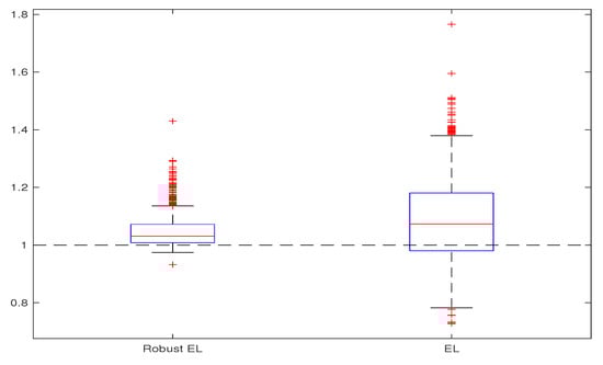
Figure 1.
Robust EL versus EL, for and .
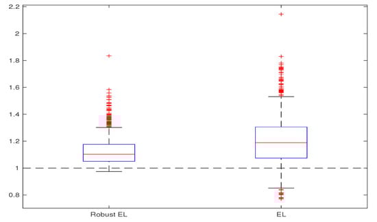
Figure 2.
Robust EL versus EL, for and .
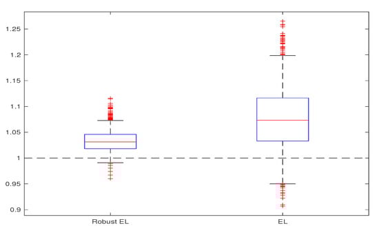
Figure 3.
Robust EL versus EL, for and .
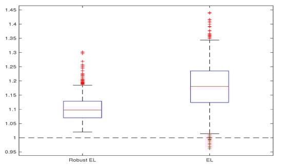
Figure 4.
Robust EL versus EL, for and .

Table 1.
Robust Empirical Likelihood (EL) versus EL, for and .
Table 2.
Robust EL versus EL, for and .
Table 3.
Robust EL versus EL, for and .
Table 4.
Robust EL versus EL, for and .
4. Conclusions
We proposed a robust version of the EL estimator for moment condition models. This estimator is defined through the minimization of an empirical version of the modified Kullback–Leibler divergence in dual form, using truncated orthogonality functions based on multivariate Huber function. We proved the robustness by means of the influence function, as well the consistency of the new estimator. The results of the Monte Carlo simulation study show that, in the case of contaminated data, the robust EL estimator outperforms the classical EL estimator.
Author Contributions
Conceptualization, A.K. and A.T.; methodology, A.K. and A.T.; investigation, A.K. and A.T.; writing the manuscript, A.K. and A.T. All authors have read and agreed to the final version of the manuscript.
Funding
This work was supported by a grant of the Romanian Ministery of Education and Research, CNCS—UEFISCDI, project number PN-III-P4-ID-PCE-2020-1112, within PNCDI III.
Institutional Review Board Statement
Not applicable.
Informed Consent Statement
Not applicable.
Data Availability Statement
Not applicable.
Conflicts of Interest
The authors declare no conflict of interest.
References
- Hansen, L.P. Large sample properties of generalized method of moments estimators. Econometrica 1982, 50, 1029–1054. [Google Scholar] [CrossRef]
- Hansen, L.P.; Heaton, J.; Yaron, A. Finite-sample properties of some alternative generalized method of moments estimators. J. Bus. Econ. Stat. 1996, 14, 262–280. [Google Scholar]
- Qin, J.; Lawless, J. Empirical likelihood and general estimating equations. Ann. Stat. 1994, 22, 300–325. [Google Scholar] [CrossRef]
- Imbens, G.W. One-step estimators for over-identified generalized method of moments models. Rev. Econ. Stud. 1997, 64, 359–383. [Google Scholar] [CrossRef]
- Owen, A. Empirical Likelihood; Chapman and Hall: New York, NY, USA, 2001. [Google Scholar]
- Kitamura, Y.; Stutzer, M. An information-theoretic alternative to generalized method of moments estimation. Econometrica 1997, 65, 861–874. [Google Scholar] [CrossRef]
- Imbens, G.W. Generalized method of moments and empirical likelihood. J. Bus. Econ. Stat. 2002, 20, 493–506. [Google Scholar] [CrossRef]
- Newey, W.K.; Smith, R.J. Higher order properties of GMM and generalized empirical likelihood estimators. Econometrica 2004, 72, 219–255. [Google Scholar] [CrossRef]
- Ronchetti, E.; Trojani, F. Robust inference with GMM estimators. J. Econom. 2001, 101, 37–69. [Google Scholar] [CrossRef]
- Lô, S.N.; Ronchetti, E. Robust small sample accurate inference in moment condition models. Comput. Stat. Data Anal. 2012, 56, 3182–3197. [Google Scholar] [CrossRef]
- Felipe, A.; Martin, N.; Miranda, P.; Pardo, L. Testing with exponentially tilted empirical likelihood. Methodol. Comput. Appl. Probab. 2018, 20, 1–40. [Google Scholar] [CrossRef]
- Broniatowski, M.; Keziou, A. Divergences and duality for estimation and test under moment condition models. J. Stat. Plan. Inference 2012, 142, 2554–2573. [Google Scholar] [CrossRef]
- Broniatowski, M.; Keziou, A. Parametric estimation and tests through divergences and the duality technique. J. Multivar. Anal. 2009, 100, 16–36. [Google Scholar] [CrossRef]
- Toma, A.; Leoni-Aubin, S. Robust tests based on dual divergence estimators and saddlepoint approximations. J. Multivar. Anal. 2010, 101, 1143–1155. [Google Scholar] [CrossRef]
- Toma, A.; Broniatowski, M. Dual divergence estimators and tests: Robustness results. J. Multivar. Anal. 2011, 102, 20–36. [Google Scholar] [CrossRef]
- Toma, A. Model selection criteria using divergences. Entropy 2014, 16, 2686–2698. [Google Scholar] [CrossRef]
- Schennach, S.M. Point estimation with exponentially tilted empirical likelihood. Ann. Stat. 2007, 35, 634–672. [Google Scholar] [CrossRef]
- Toma, A. Robustness of dual divergence estimators for models satisfying linear constraints. C. R. Math. 2013, 351, 311–316. [Google Scholar] [CrossRef]
- Engle, R.F. Autoregressive conditional heteroscedasticity with estimates of the variance of United Kingdom inflation. Econometrica 1982, 50, 987–1007. [Google Scholar] [CrossRef]
- Bansal, R.; Hsieh, D.; Viswanathan, S. No arbitrage and arbitrage pricing: A new approach. J. Financ. 1993, 48, 1719–1747. [Google Scholar] [CrossRef]
- Hampel, F.R.; Ronchetti, E.M.; Rousseeuw, P.J.; Stahel, W.A. Robust Statistics: The Approach Based on Influence Functions; Wiley Series in Probability and Mathematical Statistics: Probability and Mathematical Statistics; John Wiley & Sons Inc.: New York, NY, USA, 1986. [Google Scholar]
- Rüschendorf, L. On the minimum discrimination information theorem. Stat. Decis. 1984, 1984 (Suppl. 1), 263–283. [Google Scholar]
- Cressie, N.; Read, T.R.C. Multinomial goodness-of-fit tests. J. R. Stat. Soc. Ser. B 1984, 46, 440–464. [Google Scholar] [CrossRef]
- Broniatowski, M.; Keziou, A. Minimization of ϕ-divergences on sets of signed measures. Stud. Sci. Math. Hung. 2006, 43, 403–442. [Google Scholar]
- Basu, A.; Harris, I.R.; Hjort, N.L.; Jones, M.C. Robust and efficient estimation by minimizing a density power divergence. Biometrika 1998, 85, 549–559. [Google Scholar] [CrossRef]
- She, Y.; Owen, A. Outlier detection using nonconvex penalized regression. J. Am. Stat. Assoc. 2011, 106, 626–639. [Google Scholar] [CrossRef]
- van der Vaart, A. Asymptotic Statistics; Cambridge University Press: Cambridge, UK, 1998. [Google Scholar]
- Newey, W.K. Uniform convergence in probability and stochastic equicontinuity. Econometrica 1991, 59, 1161–1167. [Google Scholar] [CrossRef]
Publisher’s Note: MDPI stays neutral with regard to jurisdictional claims in published maps and institutional affiliations. |
© 2021 by the authors. Licensee MDPI, Basel, Switzerland. This article is an open access article distributed under the terms and conditions of the Creative Commons Attribution (CC BY) license (https://creativecommons.org/licenses/by/4.0/).