Abstract
In this paper, we computed general interval indicators of availability and reliability for systems modelled by time non-homogeneous semi-Markov chains. First, we considered duration-dependent extensions of the Interval Reliability and then, we determined an explicit formula for the availability with a given window and containing a given point. To make the computation of the window availability, an explicit formula was derived involving duration-dependent transition probabilities and the interval reliability function. Both interval reliability and availability functions were evaluated considering the local behavior of the system through the recurrence time processes. The results are illustrated through a numerical example. They show that the considered indicators can describe the duration effects and the age of the multi-state system and be useful in real-life problems.
1. Introduction
Reliability measures of repairable systems have been extensively investigated. Specific indicators are used according to the characteristics of the system that the user wishes to understand and to the nature of the system. For example, it is common to come across reliability, availability, and maintainability functions when dealing with general mechanical systems (see, e.g., [1]) or to single-use reliability function for software performance assessment (see, e.g., [2,3]). Frequently, the evolution of the system is conveniently described by multi-state models where the state of the system evolves in time according to a specified probabilistic structure (see, e.g., [4]). One of the most popular choices is for Markov chain models in continuous or discrete-time cases (see, e.g., [5]). Markov models rely on the Markovian property that informally states that the future state of a system is independent of its past evolution given the state occupied at present. Unfortunately, this property is rarely observed on real data in reliability studies as well as in different domains of applications. For this reason, the proposal of more general frameworks is becoming, even more, a rule rather than an exception. This is confirmed by the success achieved by semi-Markov models in different scientific domains such as applied probability [6], financial credit ratings [7], population dynamics [8], asymptotic behavior of random systems [9] risk assessment and evaluation [10], change of measures in credit risk [11] and pricing problems [12].
Semi-Markov processes have been applied in reliability studies by several authors. Studies based on discrete-time semi-Markov processes in homogeneous case (see e.g., [13]) and in the non-homogeneous case (see e.g., [14]) have demonstrated the ability of this class of stochastic processes to describe and represent problems of reliability theory in a more flexible and satisfactorily way as compared to Markovian models. Continuous-time models were considered in [15] as related to the dependability analysis of a semi-Markov system, in [16] for numerical treatment of probabilistic functions in homogeneous case and in [17] for non-homogeneous processes. Models with general state space related to reliability measures were considered in [18] and existence and uniqueness of solutions of Markov renewal equations were investigated in [19]. Recent developments concern indexed semi-Markov models [20] and the development of reliability measures for those systems showing the presence of an indexed mechanism [21].
In a semi-Markov processes, the transition probabilities and related indicators are duration dependent, that is, the time the system is in a state influence its transition probabilities, see e.g., [22,23]. This effect can be shown by computing transition probabilities including the information contained in the recurrence time processes. Recurrence time processes play an important role in describing the local behavior of a renewal process, see e.g., [24]. They are also intimately related to semi-Markov processes which are a multivariate extension of renewal processes. For this reason, they have been investigated by many authors both connected to the asymptotic behavior of the process ([25,26]) as well as to the transient analysis, see e.g., [27]. The recurrence times are of a backward and forward type. The former denotes the time since the last transition of a system or, in other words, the time elapsed in the current state occupied by the system. The latter denotes the time to the next transition. The reason for the existence of this duration dependence resides in the fact that the conditional waiting time distribution functions in the states of the system, i.e., the length of time in a state before making a transition, can be of any type, furthermore, no memoryless distributions can be used. In this case, the time length spent in the starting state (backward value) changes the transition probabilities as well as the information concerning how long the process will stay in the current state (forward value). The consideration of backward and forward processes at the initial and final times permits us to have complete knowledge of the waiting times at the beginning and at the end of the observation period of the model, this issue has been investigated in discrete time [22], continuous time models [23] and related to the mono-unireducible topological structure [28].
Recently, a stream of research has focused on general performance measures of a system. The proposed measures generalize classical reliability indicators. These measures are interval based in the sense that they refer to properties of the system not in relation to a point in time but rather to an interval of time.
Confining our attention to semi-Markov systems, the first contributions dealing with interval measures, in the specific with the interval reliability, are those by [29,30]. In those papers, the author determines a system of integral equation the interval reliability function should satisfy. The solution gives the probability of the system to be operational in a given time interval originating at some time and length . This measure contains, as special cases, the availability function and the reliability function and has also been evaluated concerning discrete-time systems, see [31,32]. Similar ideas are at the origin of another interval-based measure: the availability of a given window and containing a point. This function is defined as the probability that a repairable system is operational throughout an interval window of length which contains a point in time . This interval availability function has been introduced by [33] for Markov repairable systems in continuous-time and successively generalized by [34] for discrete-time semi-Markovian systems. The results are achieved by determining specific relations concerning the Z-transform of working period length, failure period length and whole period length. These Z-transforms are used to get a representation of the corresponding Z-transforms of reliability and availability measures and need the application of inverse Z-transforms to produce numerical results.
In the present paper, we considered several new aspects in the computation of interval-based performability indices. First, we extended the framework from time-homogeneous processes to a more general time non-homogeneous setting. In our case, the indicators depend on the initial time when the evaluation is done. Accordingly, the age of the system is fully taken into account. Second, we computed the indicators involving the recurrence time processes at the initial time. This extension allows us to consider the duration effect properly. Third, we provided a new proof of the availability of a given window and containing a point that does not make use of transform analysis. The proof is based on the introduction of specific random times and on the exploration of the relationship among duration dependent transition probability function, duration-dependent interval reliability and availability of given window. The result is a new formula linking the aforementioned indicators.
The next section contains a short description of discrete-time non-homogeneous semi-Markov processes with recurrence time processes. The section after presents the main results of the paper. First, the general framework of performability analysis through multi-state systems is presented together with classical reliability indicators. Then, the Duration Dependent Interval Reliability function is presented and explicit formulas are given for its calculation in different cases. The section ends by considering the Duration Dependent Availability of given window and containing a point and a new relation that can be used for its computation. Section 4 presents an example of a repairable semi-Markov system for which all of the considered performance measures are evaluated. In the last section, some concluding remarks are made.
2. Non-Homogeneous Semi-Markov Models
In this section, discrete-time semi-Markov models are briefly described. Let be a probability space equipped with a filtration satisfying the usual conditions. On this probability space, we defined two random variables denoted by and . The variable , represents the state of the system at the n-th transition and assumes values in a finite state space E = {1, 2, …, m}. The random variable , , with state space equal to , represents the time of the n-th transition. The filtration coincides with the natural filtration generated by the joint process . The process is supposed to be a non-homogeneous discrete-time Markov Renewal Process. Accordingly, we assume that:
The probabilities define the so-called semi-Markov kernel. They can be written as follows:
The main difference between a non-homogeneous Markov process and a non-homogeneous semi-Markov process (NHSMP) resides in the family of probability distributions . Indeed, in a Markovian framework, these functions have to be geometrically distributed, while, in the semi-Markov case they can be of any type. The probabilities represent the transition probabilities of the non-homogeneous embedded Markov chains . They denote the probability to have next transition in state j given that the system entered state i at current time s.
Now, let be the number of transitions up to time t, then the discrete-time non-homogeneous semi-Markov chain is defined according to:
The process indicates which state is being to be occupied by the embedded Markov chain at the last transition.
Transition probability functions are defined in the following way:
Hence, they denote the probability of being in state at time given that the system entered state at time . They are obtained by solving the following evolution equations, see e.g., [21]:
where is the Kronecker’s delta, and
The first part on the right-hand side (RHS) of Equation (1) expresses the probability the system does not have any transition up to the time conditional on the entrance in the state at the time . The second term represents the probability that the system will enter into state at time , given that it entered the state at time and then, after the execution of this transition, will follow one of the possible trajectories connecting state at time , to state at . This event is considered for all possible values of and .
Given the process , it is possible to introduce two stochastic processes of recurrence times: the backward process and the forward process They are defined according to:
Following the general notation adopted in [22] we consider some transition probability functions with recurrence time processes that will be needed to reach our scopes. First, define by:
We call Equation (3) the transition probability functions with initial backward and forward. These probabilities can be obtained according to the following equation:
Equation (4) reveals that the probability to be in state at time depends on the local behavior of the process in the initial time , i.e., on the state occupied at that time and also on the time since last jump and on the time needed to have next transition. The transition probabilities in (4) can be obtained once Equation (3) is solved. Particular cases of Equation (4) are those where the recurrence time processes are considered separately. Precisely, we can have transition probability with initial backward
which satisfy relation:
with , and transition probability with initial forward:
which satisfy formula:
The last probability of our interest is the one with initial and final backward times, i.e.,
which satisfy relation:
and .
All of the relations presented before are particular cases of the more general transition probability functions with initial and final backward and forward presented in [22].
3. Interval-Based Performability Measures
In this section, we present the main results of the paper. First, we described the framework of multistate systems as applied to reliability studies, and successively, we analyzed two performability measures for a repairable system based on semi-Markov process and we derived specific recurrent relations useful for their computation.
3.1. The General Framework of Performability Analysis through Multi-State Systems
A general approach to measure the performance of a system is to consider a state space E = {1, 2, …, m} as a representation of the different levels to which a system can perform. In some circumstances, it may be opportune to assume an ordering relation on E so that to lower ranks correspond to a lower system’s performance. It is frequent to partition the state space E into two disjoint sets and such that:
The subset contains all the elements of which denote that the system is operational (or working well), instead the subset contains all the states of in which the system is not well performing or has fault. The system changes its performance in time by migrating from one state to another. According to our working hypothesis, we assume the stochastic behavior of the system can be well represented by a non-homogeneous discrete-time semi-Markov process .
The overall quality of the system can be measured by introducing specific indicators that we need to remember in a non-homogeneous environment.
The availability function for a non-homogeneous semi-Markov system can be defined by:
This function expresses the probability that a system ranked i at time s will be operational at time t. This indicator can be computed using the following formula:
The reliability function for a non-homogeneous semi-Markov system can be defined by:
This function expresses the probability that a system ranked i at time s will never experience a fault (visit to subset ) from time s up to time t. This indicator has been evaluated through a transformation of the semi-Markov kernel that render the states of absorbing. In formula:
where are the transition probabilities computed by using the following kernel transformation:
The transformation (15) defines a new semi-Markov kernel for which all the states of the subset D are changed in absorbing states, see [14].
The availability and the reliability functions have also been generalized by considering the influence of the recurrence time processes and as developed for example in [22].
3.2. The Duration Dependent Interval Reliability Function
The notion of Interval Reliability has been introduced for continuous-time semi-Markov processes in [29,30] and only recently it has been investigated in relation to discrete–time semi-Markov processes in [31,32]. In this subsection, we extended this indicator to the more general non-homogeneous discrete-time semi-Markov framework and we derived formulas that consider the influence of recurrence time processes in different ways.
First, we defined the Non-Homogeneous Interval Reliability , as the probability that the system is working at time t and will continue to work for the next time units given that at time the system entered state . In formula:
This measure is of particular interest and includes as special cases both the reliability and availability function. In this regard, it is sufficient to observe that:
The calculation strategy adopted in [31] can be adjusted to the time non-homogeneous processes. Thus, it is possible to obtain the following relation:
It should be remarked that Equation (16) is of recursive type and can be seen as a Markov Renewal Equation for which well-known computational methods have been proposed to get a solution. The seminal contribution of Erhan Çinlar [26] was followed by an extensive treatment in [27] and some recent results given in [19]. Numerical methods were developed in [35] while general indexed Markov renewal equations were considered in [20] together with their numerical solution.
Now, we proceed to compute the Interval Reliability using the incremental information brought by the recurrence time processes in different cases. To this end, we define the Duration Dependent Interval Reliability , as the probability that the system is working at time and will continue to work for the next time units given that at time the system occupies state being entered in this state in the last transition at time and will exit from this state at time . In formula:
Thus, this function expresses the probability of the same event considered by but evaluated on an enlarged information set which includes local behavior of the system around the present time . Any difference between is only due to the influence of the recurrence time processes at the initial time .
It should be remarked that while the event the same does not hold for which is not -measurable. Accordingly, the conditioning at time on possible values of the forward process may serve as a strategy to build scenario-based perturbations of a reliability indicator.
A slightly more general indicators can be defined allowing for the process to assume value in a specified time interval, namely . This motivates the following definition.
The Duration Dependent Interval Reliability , is defined as the probability that the system is working at time and will continue to work for the next time units given that at time the system occupies state being entered in this state in the last transition at time and will exit from this state in a moment belonging to the time interval . In formula:
It is simple to realize that .
The following proposition provides formulas for computing the Duration Dependent Interval Reliability according to five different cases we can observe according to the diverse relationship between temporal variables.
Proposition 1.
The Duration Dependent Interval Reliabilityfor a discrete-time non-homogeneous semi-Markov system can be expressed by the following six cases:
- (i)
- Forwe can prove that:
- (ii)
- Forwe have that:Forit results that:
- (iii)
- Forwe have that:
- (iv)
- For
- (v)
- For
Proof.
We start with the proof of Equation (17) which corresponds to the case when . In this eventuality it results that:
The denominator of Equation (23) is given by:
The numerator of Equation (23) is given by:
A substitution of Equations (24) and (25) in Equation (23) gives Equation (9).
Equation (18) corresponds to the case when . Let us consider again Equation (23):
The denominator has been calculated in Equation (24), whereas the numerator can now be represented as follows:
A substitution of Equations (24) and (26) in Equation (23) gives Equation (18).
Equation (19) corresponds to the case when . Let us consider again Equation (23):
The denominator has been calculated in Equation (24), whereas the numerator can be now represented as follows:
A substitution of Equations (24) and (27) in Equation (23) gives Equation (19).
Equation (20) corresponds to the case when . Let us consider again Equation (23):
The denominator has been calculated in Equation (24), whereas the numerator can be now represented as follows:
A substitution of Equations (24) and (28) in Equation (23) gives Equation (20).
Equation (21) corresponds to the case when . The starting point is always Equation (23) for which the denominator has been calculated in Equation (24). The numerator can be now represented as follows:
Now, due to the ordering relation among the considered times we write the former probability as follows:
A substitution of Equations (24) and (29) in Equation (23) gives Equation (21).
Equation (22) corresponds to the case when . In this case, directly from the definition of the Duration Dependent Interval Reliability we get:
because implies that □
Corollary 1.
The Duration Dependent Interval Reliability for a discrete-time non-homogeneous semi-Markov system can be expressed by the following three cases:
- (i)
- Forwe have that:
- (ii)
- Forwe have that:
- (iii)
- Forwe have that:
Proof.
Equation (30) is obtained simply considering Equation (22) with .
Equations (31) and (32) are obtained from Equations (20) and (18) with and observing that in this case we obtain:
□
The Duration Dependent Interval Reliabilities and provide important information to the reliability engineer. In particular, the backward value at initial time permits to include in the model the information related to the time occupancy of the current state of performance of the system. This allows the possibility to differentiate the evaluation of the reliability of the system according to the time elapsed in the current state. This feature is a prerogative of the semi-Markovian models and cannot be reproduced by Markov chain based models. The indicator considers also the impact of the value of the forward process at time and permits the measurement of the effect caused by the time in which the first transition after the current time will happen. Since this time cannot be known at the present time , any conjecture on its value can be used to build up a scenario analysis of the reliability of the system. Due to the uncertainty on the value of the forward process, the indicator permits the advancement of even mild belief on the value of which can now be expressed in interval form. All of the obtained relations (Equations (18)–(32)) express the Duration Dependent Interval Reliabilities as a function of the Reliability and Interval Reliability of the system.
3.3. The Duration Dependent Availability of Given Window and Containing a Point
In this subsection, we dealt with another performability measure based on intervals. In particular, we considered the availability of a given window and containing a point. This measure has been introduced for Markov repairable stochastic systems in [33] where the corresponding calculation formula is derived using the Laplace transform technique. A further generalization is provided in [34] where the analysis is extended to discrete-time homogeneous semi-Markov systems. Again the results are obtained using the mathematical apparatus based on transform analysis which requires inverse transformation to get numerical results useful in applications. Here, we extended the investigation to include non-homogeneous discrete-time semi-Markov process with duration dependence effects. We demonstrated how to derive a formula for this indicator without making use of transform analysis and exploiting the relationship between this indicator, the Duration Dependent Interval Reliability and the duration dependent transition probability function To achieve this result we needed to introduce the formal definition of the indicator, some auxiliary random times, and corresponding properties.
We defined the Duration Dependent Availability of the given window and containing a point , as the probability that a repairable system works throughout an interval window which has at least a length and contains a given point given that at time the system was in state with a time elapsed in this state equal to . In formula:
We defined the last failure time before time as:
with the convention that when .
We also defined the excess time of at the level as the random variable defined according to:
It denotes the minimum time to add to to reach at least the length .
Let us introduce two useful subsets of the sample space that are in a direct relation with and .
First we denote by:
and then consider the set:
Lemma 1.
The subsetsandsatisfy the following relation:
Proof.
Given three times we can distinguish two cases:
Let us first consider the case a). In order to represent the set in this situation we can enumerate all the intervals where the system works. The first interval is which is equal to with The second interval is , i.e., the interval with The latter is the interval , i.e., the interval for Thus, the union of all these intervals gives:
Set to transform Equation (40) into:
In the alternative case b), that is when the enumeration of all possible intervals of length covering starts from the first interval which is obtained for and proceeds until the last interval which is obtained for Thus, the union of all these intervals gives:
that, after the change of variable is transformed into:
Equations (41) and (43) can be merged using the max and min operators in a unique expression:
□
Lemma 2.
The subsetsandsatisfy the following relation:
Proof.
Fix the three times such that and and observe that from Lemma 1 we have that:
Observe now that for :
whereas for :
then by substitution, Equation (45) becomes:
A change of variable posing transforms Equation (47) into:
which proves the first part of Equation (44).
Let us consider now the second case which corresponds to times such that and .
From Lemma 1 we have that:
Now, observe that:
Moreover, from Equation (46) we have:
Therefore:
Now, set then Equation (49) becomes equal to:
In this way by substitution, we obtain that for , is expressed by the union between the sets, i.e.,
□
Proposition 2.
The Duration Dependent Availability of given window and containing a pointfor a discrete-time non-homogeneous semi-Markov system can be expressed by the following formula:
Proof.
The Duration Dependent Availability of given window and containing a point can be expressed in term of the set
where the last equality is only considered for introducing a compact notation we shall use extensively. First, consider that:
Consider before the first addendum of Equation (51)
Now, we distinguish two cases according to whether or If from Lemma 1 we know that and then we have that:
Consequently, the first term on the RHS of Equation (52) becomes:
While:
On the contrary, for from Lemma 1 we know that and since:
we have that:
Thus, the results obtained in the two cases give:
It still remains to compute the second addend on the RHS of Equation (51). We proceed by decomposing it according to Lemma 2 as follows:
The events are mutually exclusive for any choice of or . Thus, we get
Now, let us consider the first addendum on the RHS of Equation (55):
where the symbol denotes the set of possible durations (value of the backward process) at time Equation (56) can be expressed as follows:
Now, notice that:
- (i)
- (ii)
- where the first equality is due to the Markovian property of the joint process .
- (iii)
- In the case , by definition of the backward process we have that which means that from time to time no change of state is allowed. Accordingly, state should coincide with state Formally:
- (iv)
Then, a substitution of the quantities computed in the points (i)–(iv) inside Equation (57) gives the following representation of the first addendum on the RHS of Equation (47):
Now, we proceed to compute the second addendum on the RHS of Equation (55). The computations share similar ideas as those generating Equation (58). In particular:
Finally, we can compute the third addendum on the RHS of Equation (55). The computations are based again on similar ideas as those which gave Equation (58). In particular:
We observed that Equations (58) and (60) may be merged in a unique expression because the indicator function in Equation (60) implies that:
Concerning Equation (58), due to the fact that , it can be rewritten replacing the summation as follows:
According to Equations (61) and (62), we can write the summation of Equations (58) and (60) by:
A substitution of (59) and (63) in (55) and the summation of the results with (54) completes the proof. □
4. A Numerical Example
In this section, we gave a numerical example of the behavior of the Duration Dependent Interval Reliability functions and of the Duration Dependent Availability.
To simplify this application, we considered a repairable systems with only two states for the system: state and state . When the system is in state it means that it is working, on the contrary state denotes a failure of the system. We modelled an non-homogeneous semi-Markov kernel by fixing a transition probability matrix which makes provision for a system alternating its states between state and state according to the following transition probability matrix:
and time varying sojourn time distributions according to Weibull distribution:
with time-varying parameters given by:
In this way, we were able to model a non-homogeneous semi-Markov process. Then, we used the theoretical relations determined in previous sections to compute the Non-Homogeneous Interval Reliability, the Duration Dependent Interval Reliability and the Duration Dependent Availability of the given window and containing a point. The results have been validated implementing a Monte Carlo technique based on 100,000 simulated trajectories. The algorithm to simulate the process is described in Figure 1.
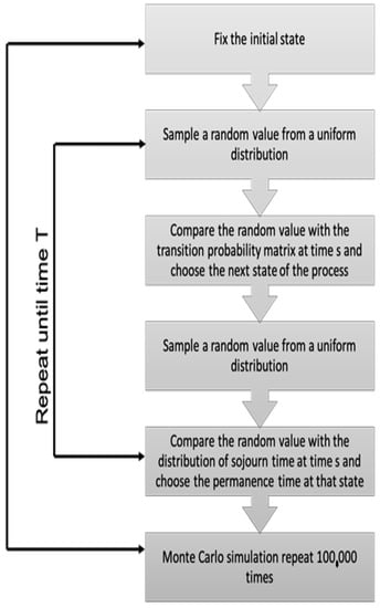
Figure 1.
Algorithm for the simulation of non-homogeneous semi-Markov trajectories.
In Figure 2 we plotted the Non-Homogeneous Interval Reliability for initial state and , for reference purpose we set . The behavior is as expected, in fact the probability to work for time length is inversely proportional to itself in both cases, but it is inversely proportional to when the system is already in state while the proportionality with respect to is the opposite when the starting state is .
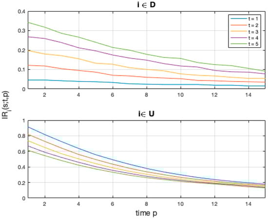
Figure 2.
Non-Homogeneous Interval Reliability. For reference purpose we fixed s = 0.
In Figure 3, we show the Duration Dependent Interval Reliability for some fixed values of parameters. Specifically, we set and let change possible values of the forward interval and selected four different values of . Also, in this case, we can see that the probability is higher for lower values of , another important feature is that the probability does depend on the forward time in the interval .
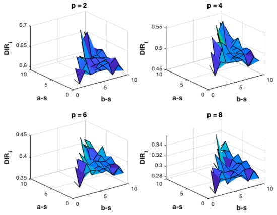
Figure 3.
Duration dependent Interval Reliability. In the plots, i = U, s-l = 3, and t = 10.
The Duration Dependent Availability of the given window and containing a point is shown in Figure 4 for . The function is plotted depending of and . As expected, the probability decreases when the window length increases. We also found a small dependence on . In fact, for small values and for high values of the probability is higher.
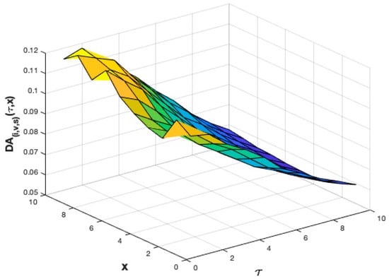
Figure 4.
Duration dependent Availability, i = U, v = 3, and s = 0.
5. Conclusions
In this paper, we extended the definition of some important reliability indicators in several directions. First, we considered a discrete-time non-homogeneous semi-Markov repairable model for which interval availability and reliability indicators are defined in such a way to consider the durational effects in terms of backward and forward recurrence time processes. Then, we analysed the link between these indicators and previously studied measures and we determined new formulas of recurrence type useful to the computation of the new indexes. The results avoid the recourse to the transform analysis apparatus and may be applied in real life problems of reliability. Further developments of this research include the extension of the analysis to indexed semi-Markov models and the application of the results to other applied domains such as finance and renewable energies. A possible further extension consists of the computation of these measures when some of the parameters of the reliability system are expressed in form of intervals. It is not infrequent, in the study of a mechanical system, to improve performance evaluation of uncertain systems using interval parameters, see e.g., [36]. Thus, a mixed form of uncertainty can be considered both probabilistic and engineering in nature.
Author Contributions
Conceptualization, G.D., R.M. and D.S.; methodology, G.D.; software, F.P.; validation, G.D. and D.S.; formal analysis, G.D.; investigation, G.D.; data curation, F.P.; writing—original draft preparation, G.D. and F.P. Writing—review & editing G.D, F.P. and D.S. All authors have read and agreed to the published version of the manuscript.
Funding
This research received no external funding.
Institutional Review Board Statement
Not applicable.
Informed Consent Statement
Not applicable.
Data Availability Statement
Data is contained within the article.
Conflicts of Interest
The authors declare no conflict of interest.
References
- Barbu, V.S.; Limnios, N. Semi-Markov Chains and Hidden Semi-Markov Models toward Applications: Their Use in Reliability and DNA Analysis; Springer Science & Business Media: Berlin/Heidelberg, Germany, 2008; Volume 191. [Google Scholar]
- Prowell, S.; Poore, J. Computing system reliability using Markov chain usage models. J. Syst. Softw. 2004, 73, 219–225. [Google Scholar] [CrossRef]
- D’Amico, G. Single-use reliability computation of a semi-Markovian system. Appl. Math. 2014, 59, 571–588. [Google Scholar] [CrossRef]
- Lisnianski, A.; Frenkel, I.; Ding, Y. Multi-State System Reliability Analysis and Optimization for Engineers and Industry Managers; Springer: London, UK, 2010. [Google Scholar]
- Balakrishnan, N.; Limnios, N.; Papadopoulos, C. Ch. 1. Basic probabilistic models in reliability. In Handbook of Statistics; Elsevier: Amsterdam, The Netherlands, 2001; Volume 20, pp. 1–42. [Google Scholar]
- Janssen, J.; Manca, R. Applied Semi-Markov Processes; Springer: New York, NY, USA, 2006. [Google Scholar]
- D’Amico, G.; Di Biase, G.; Janssen, J.; Manca, R. Semi-Markov Migration Models for Credit Risk; Wiley-ISTE: London, UK, 2017. [Google Scholar]
- Vassiliou, P.-C.G.; Papadopoulou, A.A. Non-homogeneous semi-Markov systems and maintainability of the state sizes. J. Appl. Probab. 1992, 519–534. [Google Scholar] [CrossRef]
- Papadopoulou, A.; Vassiliou, P.-C. Asymptotic behavior of nonhomogeneous semi-Markov systems. Linear Algebra Its Appl. 1994, 210, 153–198. [Google Scholar] [CrossRef]
- D’Amico, G.; Manca, R.; Salvi, G. Bivariate Semi-Markov Process for Counterparty Credit Risk. Commun. Stat. Theory Methods 2014, 43, 1503–1522. [Google Scholar] [CrossRef]
- Vassiliou, P.-C. Non-Homogeneous Semi-Markov and Markov Renewal Processes and Change of Measure in Credit Risk. Mathematics 2020, 9, 55. [Google Scholar] [CrossRef]
- Silvestrov, D.; Stenberg, F. A Pricing Process with Stochastic Volatility Controlled by a Semi-Markov Process. Commun. Stat. Theory Methods 2004, 33, 591–608. [Google Scholar] [CrossRef]
- Barbu, V.; Boussemart, M.; Limnios, N. Discrete-Time Semi-Markov Model for Reliability and Survival Analysis. Commun. Stat. Theory Methods 2004, 33, 2833–2868. [Google Scholar] [CrossRef]
- Blasi, A.; Janssen, J.; Manca, R. Numerical Treatment of Homogeneous and Non-homogeneous Semi-Markov Reliability Models. Commun. Stat. Theory Methods 2004, 33, 697–714. [Google Scholar] [CrossRef]
- Limnios, N. Dependability analysis of semi-Markov systems. Reliab. Eng. Syst. Saf. 1997, 55, 203–207. [Google Scholar] [CrossRef]
- Mercier, S. Numerical Bounds for Semi-Markovian Quantities and Application to Reliability. Methodol. Comput. Appl. Probab. 2007, 10, 179–198. [Google Scholar] [CrossRef]
- Moura, M.D.C.; Droguett, E.L. Mathematical formulation and numerical treatment based on transition frequency densities and quadrature methods for non-homogeneous semi-Markov processes. Reliab. Eng. Syst. Saf. 2009, 94, 342–349. [Google Scholar] [CrossRef]
- Limnios, N. Reliability Measures of Semi-Markov Systems with General State Space. Methodol. Comput. Appl. Probab. 2011, 14, 895–917. [Google Scholar] [CrossRef]
- Hou, Y.; Limnios, N.; Schön, W. On the Existence and Uniqueness of Solution of MRE and Applications. Methodol. Comput. Appl. Probab. 2017, 19, 1241–1250. [Google Scholar] [CrossRef]
- D’Amico, G. Age-usage semi-Markov models. Appl. Math. Model. 2011, 35, 4354–4366. [Google Scholar] [CrossRef]
- D׳amico, G.; Petroni, F.; Prattico, F. Reliability measures for indexed semi-Markov chains applied to wind energy production. Reliab. Eng. Syst. Saf. 2015, 144, 170–177. [Google Scholar] [CrossRef]
- D’Amico, G.; Janssen, J.; Manca, R. Initial and Final Backward and Forward Discrete Time Non-homogeneous Semi-Markov Credit Risk Models. Methodol. Comput. Appl. Probab. 2009, 12, 215–225. [Google Scholar] [CrossRef]
- D’Amico, G.; Janssen, J.; Manca, R. Duration Dependent Semi-Markov Models. Appl. Math. Sci. 2011, 5, 2097–2108. [Google Scholar]
- Heyman, D.P.; Sobel, M.J. Stochastic Models in Operations Research: Stochastic Processes and Operating Characteristics; Dover Publications, Inc.: Mineola, NY, USA, 1982; Volume 1. [Google Scholar]
- Yackel, J. Limit theorems for semi-Markov processes. Trans. Am. Math. Soc. 1966, 123, 402–424. [Google Scholar] [CrossRef]
- Çinlar, E. Markov renewal theory. Adv. Appl. Probab. 1969, 1, 123–187. [Google Scholar] [CrossRef]
- Limnios, N.; Oprişan, G. Semi-Markov Processes and Reliability Modeling; Birkhauser: Boston, MA, USA, 2001. [Google Scholar]
- D’Amico, G.; Janssen, J.; Manca, R. Monounireducible Nonhomogeneous Continuous Time Semi-Markov Processes Applied to Rating Migration Models. Adv. Decis. Sci. 2012, 2012, 1–12. [Google Scholar] [CrossRef]
- Csenki, A. On the interval reliability of systems modelled by finite semi-Markov processes. Microelectron. Reliab. 1994, 34, 1319–1335. [Google Scholar] [CrossRef]
- Csenki, A. An integral equation approach to the interval reliability of systems modelled by finite semi-Markov processes. Reliab. Eng. Syst. Saf. 1995, 47, 37–45. [Google Scholar] [CrossRef]
- Georgiadis, S.; Limnios, N. Interval reliability for semi-Markov systems in discrete time. J. Soc. Fr. Stat. 2014, 153, 152–166. [Google Scholar]
- Georgiadis, S.; Limnios, N. Nonparametric estimation of interval reliability for discrete-time semi-Markov systems. J. Stat. Theory Pr. 2015, 10, 20–39. [Google Scholar] [CrossRef][Green Version]
- Cui, L.; Chen, J.; Wu, B. New interval availability indexes for Markov repairable systems. Reliab. Eng. Syst. Saf. 2017, 168, 12–17. [Google Scholar] [CrossRef]
- Yi, H.; Cui, L.; Shen, J.; Li, Y. Stochastic properties and reliability measures of discrete-time semi-Markovian systems. Reliab. Eng. Syst. Saf. 2018, 176, 162–173. [Google Scholar] [CrossRef]
- Janssen, J.; Manca, R. Numerical Solution of non-Homogeneous Semi-Markov Processes in Transient Case. Methodol. Comput. Appl. Probab. 2001, 3, 271–293. [Google Scholar] [CrossRef]
- Cheng, J.; Liu, Z.-Y.; Tan, J.-R.; Zhang, Y.-Y.; Tang, M.-Y.; Duan, G.-F. Optimization of Uncertain Structures with Interval Parameters Considering Objective and Feasibility Robustness. Chin. J. Mech. Eng. 2018, 31, 38. [Google Scholar] [CrossRef]


Publisher’s Note: MDPI stays neutral with regard to jurisdictional claims in published maps and institutional affiliations. |
© 2021 by the authors. Licensee MDPI, Basel, Switzerland. This article is an open access article distributed under the terms and conditions of the Creative Commons Attribution (CC BY) license (http://creativecommons.org/licenses/by/4.0/).