Robust Pairwise n-Person Stochastic Duel Game

Abstract

This paper introduces an extended version of a stochastic game under the antagonistic duel-type setup. The most flexible multiple person duel game is analytically solved. Moreover, the explicit formulas are solved to determine the time-dependent duel game model using the first exceed theory in multiple game stages. Unlike conventional stochastic duel games, multiple battlefields are firstly introduced and each battlefield becomes a shooting ground of pairwise players in a multiperson game. Each player selects different targets in different game stages. An analogue of this new theory was designed to find the best shooting time within multiple battlefields. This model is fully mathematically explained and is the basis with which to apply a stochastic duel-type game in various practical applications.

1. Introduction

Game theory has been adapted to various applications in the fields of business and management, including economics, marketing, and strategic management [1,2,3]. Moreover, the domain has been expanded even further to one of most sophisticated technologies [4,5,6,7,8]. A conventional duel game is an arranged engagement in a combat situation between two players, with matched weapons, in accordance with the agreed rules under different conditions [9]. The duel-type game has evolved several extensions over the past decades [10,11,12,13,14,15]. In a versatile stochastic duel game, a joint functional of a standard stopping game is constructed to analyze the decision-making parameters in the time domain for two-players [16,17,18] and this is extended to an OneToN game system, which is a multiplayer duel game with the one-shoot-kills-all condition [19]. In this paper, another extended version of a multiperson stochastic duel game is explored by adapting multiple game stages (i.e., battlefields).

The robust method was designed for selecting the best strategies in a general antagonistic multiperson stochastic duel game. This game has multiple game stages, which are called battlefields, and each battlefield might have different pairwise players with different optimal shooting moments. Although multiple players are joined in multiple battlefields, each player only has one bullet in a single game. On their turn (or iteration), each player can choose to either “wait” for one step closer to the target or “shoot” to kill a target player. A player at a random time with random impact can take the best shooting opportunity after passing the fixed threshold, but players keep in mind that each player has only one chance to shoot someone. This newly proposed model can be used to describe various marketing and technology strategy situations (i.e, intellectual properties) in the high-tech industry domain.

Because of backward induction, a player can hit an opponent player when a certain threshold is passed. Unlike the latest versatile n-person duel game [19], each player only has one bullet and can only kill one person during a whole game. From various studies of duel-type games since the 1970s, the basic rules have never changed. The key lesson is that the best decision concerns when to act, rather than what to do [9]. The game system in this paper is the most flexible game model within the versatile stochastic duel game series [18,19]. Although the game is constructed for multiple players, shooting only happens between two players on a battlefield. Hence, the best shooting chance on each battlefield can be analyzed based on a pairwise player set, and the analysis of each pairwise player set falls into a two-person versatile duel game because of backward induction [18]. This research introduces robust approaches to determine the best player responses. The strategies for duel-type games are time sensitive and the best responses keep changing in a timely manner. Although the status of a game is changed once a player shoots a target player, the method to find the best responses for all players is recursive and essentially the same, only changing for different game statuses (i.e., the number of players and the probability of success of players who exhaust their bullets).

The paper is constructed as follows. Section 2 contains the mathematical model that analyzes the shooting order of the players in a game and the best shooting moment for each player. A joint functional of each component that describes the process at the first pass of the dominant point and at one step prior for each player is also provided in this section. In Section 3, the pairwise two-person mixed strategy in multiple game stages is applied to find the optimal mixed strategies of each set of paired players. Lastly, the conclusion is provided in Section 4. Additionally, the Matlab source codes for numerical demonstrations were developed and made publicly available for further research.

2. n-Person Stochastic Duel Game

The antagonistic stochastic n-person duel game is introduced and all pairwise players know the complete information regarding the success probabilities in each time domain battlefield. After completing each iteration, two players in each battlefield can choose either one of two strategies which are “shoot” an opponent player or “hold” until the next iteration. It is noted that each battlefield is opened with different pairwise player sets.

2.1. Preliminaries

The antagonistic duel game for n players contains the discrete random time series (i.e., iteration period). Let $A_i\left(t\right)$ be a payoff (related) function of each player $i=1,\dots ,n$ at time $t_i$ and the payoff functions of all players are assigned as follows:

$$\left\{A_i\left(t\right):0 \le A_i\left(t\right) \le A_i\left(t+\Delta \right),t\in \left[0,t_i^{\max }\right],t_i^{\max }\in {\mathbb{R}}_{+},\Delta >0\right\},$$

(1)

and these are all monotone nondecreasing functions. The accumulative success probability functions of players are determined as follows:

$$P_i\left(t\right) :=\frac{A_i\left(t\right)}{A_i\left(t_i^{\max }\right)},P_j\left(t\right) :=\frac{A_j\left(t\right)}{A_j\left(t_j^{\max }\right)},j\in -i,i=1,\dots ,n.$$

(2)

The best strategy for each player in an n-person duel game is choosing the moment to hit an opponent in a particular battlefield. As is shown in Figure 1, the accumulative success probabilities of all players are arbitrary incremental continuous functions which reach 1 when the time $t_i$ meets the allowed maximum $\left(t_i^{\max },t_{-i}^{\max }<\infty \right)$.

In duel games, a certain point $t_{\left\{i_1,j_1\right\}}^1$ maximizes the chance of a successful shot within the first pairwise players, and this best point is the first moment of success in the continuous time domain:

$$t_{\left\{i_1,j_1\right\}}^1={\mathrm{argmin}}_{t_{\left\{i,j\right\}}}\left\{t_{\left\{i,j\right\}}\ge 0 : \left\{P_{i_1}\left(t\right)-\left(1-P_{j_1}\left(t\right)\right)\ge 0\right\},j_1\in -i_1\right\},$$

(3)

where n is the number of players, which is five for our demonstration. It is noted that each player can make the decision at a certain point in time, and this is the reason why it becomes a discrete time series, despite the success probabilities being continuous functions.

For the five-person duel game in Figure 1, the first shooting paired players are players 2 and 3. The best shooting time for player 2 is 10.2 with a 60.0 percent chance of winning the first field, while player 3 has a 39.6 percent chance of winning at the same best shooting time (see Figure 2). In a five-person duel game, 10 battlefields (i.e., $m\in \left\{1,\dots ,10\right\}$) are installed and each player is involved in four battles (or games) within 10 battles. The best shooting moments of player i in the m-th battlefield can be defined as follows:

$$t_{\left\{i,j_m\right\}}^m={\mathrm{argmin}}_{t_{\left\{i,j_m\right\}}}\left\{t_{\left\{i,j_m\right\}}\ge 0 : \left\{P_i\left(t\right)-\left(1-P_{j_m}\left(t\right)\right)\ge 0\right\},j_m\in -i\right\}.$$

(4)

Each player will have three more (i.e., overall $n-1$ times) battles in which the have two-person duel games with their opponent players. In the later battlefields (i.e., $m>1$), the players should survive and hold their bullets before meeting each other. Let ($\Omega$, $\mathcal{F}$($\Omega$), P) be a probability time space and ${\mathcal{F}}_{T^i}\subseteq \mathcal{F}\left(\Omega \right)$ be independent $\sigma$-subalgebras. Suppose

$$T^i:={\sum }_{k\ge 0}{\epsilon }_{T_k^i},\left(0=\right) T_0^i<T_1^i<\dots ,i=1,\dots ,n$$

(5)

are ${\mathcal{F}}_{T^i}$-measurable renewal point processes with the following notation for players:

$${\tau }^i:=\left\{\begin{array}{cc}{\tau }_k^i=T_k^i-T_{k-1}^i,\hfill & k=1,2,\dots ,\hfill \\ 0,\hfill & k\le 0.\hfill \end{array}\right.$$

(6a)

and the functional is

$${\delta }_i\left(\theta \right)=\mathbb{E}\left[e^{-\theta {\tau }^i}\right],\mathrm{Re}\left(\theta \right)\ge 0.$$

(6b)

The stochastic game in the paper describes the evolution of conflict between players on each battlefield. To further formalize the game, the exit indices for the m-th battlefield are introduced as follows:

$${\nu }_m^i:=inf\left\{k:T_k^i=T_0^i\left(=0\right)+{\tau }_1+\cdots +{\tau }_k^i\ge U_m^i\right\},i=1,\dots ,n.$$

(7)

From Equation (4), the optimal threshold of the player i can be determined into one value in the time domain of a duel game. The player i on the m-th battlefield at $t_{\left\{i,j_m\right\}}^m$ will have the best chance of a successful shot as compared to the chance of failure of other players ($P_i\left(T_{{\nu }_m^i}^i\right)$ and $1-P_{j_m}\left(T_{{\nu }_m^{j_m}}^{j_m}\right)$, respectively). Under the situation that both players are holding their bullets until the moment of $t_{\left\{i,j_m\right\}}^m$, the player i at the m-th battlefield has the highest probability of success shooting at time $T_{{\nu }_m^i}^i$, unless player $j_m$ does not reach their best shot at time $T_{{\nu }_m^{j_m}}^{j_m}$. Thus, the game on the m-th battlefield might be ended at min$\left\{T_{{\nu }_m^i}^i,T_{{\nu }_m^{j_m}}^{j_m}\right\},$ $j_m\in -i$. However, we are targeting the confined duel game for player i on trace $\sigma$-algebra $\mathcal{F}\left(\Omega \right)\cap \left\{P_i\left(T_{{\nu }_m^i}^i\right)+P_{j_m}\left(T_{{\nu }_m^{j_m}}^{j_m}\right)\ge 1\right\}\cap \left\{T_{{\nu }_m^i}\le T_{{\nu }_m^{j_m}}\right\}$ (i.e., player i in the game obtains the best chance of shooting first). The functional for the pairwise players at a battlefield is

$$\begin{array}{cc}& {\Phi }_{{\nu }^i{\nu }^{-i}}^i={\Phi }_{{\nu }^i{\nu }^{-i}}^i\left({\theta }_0,{\theta }_1\right)=\mathbb{E}\left[e^{-{\theta }_0{S}_{\mu -1}-{\theta }_1{S}_{\mu }}·{\mathbf{1}}_{\left\{T_{{\nu }^i}\le T_{{\nu }^{-i}}\right\}}{\mathbf{1}}_{\left\{P_i\left(t\right)\ge 1-P_{-i}\left(t\right)\right\}}\right],\hfill \end{array}$$

(8)

$$\begin{array}{cc}& Re\left({\theta }_0\right)>0,Re\left({\theta }_1\right)>0,\hfill \end{array}$$

(9)

where

$${\nu }^i:={\nu }_m^i,{\nu }_m^{-i}:=\left\{{\nu }_m^{j_m}:j_m\in -i_m\right\}.$$

(10)

The game will represent the status of player i on the m-th battlefield $t_{\left\{i,j_m\right\}}^m$ and an opponent player upon the exit time $T_{{\nu }_m^i}^i$ and the pre-exit time $T_{{\nu }_m^i-1}^i$ [18]. The Laplace–Carson transform is applied as follows:

$${\widehat{\mathcal{L}}}_{pq}\left(•\right)\left(u,v\right)=uv{\int }_{p=0}^{\infty }{\int }_{p=0}^{\infty }{e}^{-up-vq}\left(•\right)d\left(p,q\right),\mathrm{Re}\left(u\right)>0,\mathrm{Re}\left(v\right)>0,$$

(11)

with the inverse

$${\widehat{\mathcal{L}}}_{uv}^{-1}\left(•\right)\left(p,q\right)={\mathcal{L}}^{-1}\left(•\frac{1}{uv}\right)$$

(12)

and

$${\widehat{\mathcal{L}}}_{uv}^{-1}\left(•\right)\left(r\right)={\widehat{\mathcal{L}}}_{uv}^{-1}\left(•\right)\left(p,q\right){|}_{\left(p,q\right)\left(r,r\right)},$$

(13)

where ${\mathcal{L}}^{-1}$ is the inverse of the bivariate Laplace transform [18]. The functional ${\Phi }_{{\nu }_m^i{\nu }_m^{-i}}^m$ for player i on the m-th battlefield in the game satisfies the following formula:

$${\Phi }_{{\nu }_m^i{\nu }_m^{-i}}^m={\widehat{\mathcal{L}}}_{uv}^{-1}\left(\mathbb{E}\left[\frac{\left(1-{\gamma }_0\left(\tau \right)\right)\left(1-{\Gamma }_0\left(\sigma \right)\right)}{{\gamma }_1\left(\tau \right)\left(1-{\gamma }_2\left(\tau \right)\right){\Gamma }_1\left(\sigma \right)\left(1-\Gamma \left(\sigma \right)\right)}\right]\Gamma \left(t_m^i\right)\right)\left(t_m^i\right),$$

(14)

where

$$\left(t_{j_m}^m=\right)t_i^m:=t_{\left\{i,j_m\right\}}^m$$

(15)

$$\gamma \left(x,t\right) = e^{-xt},$$

(16)

$$\gamma \left(t\right) :=\gamma \left(v,t\right),$$

(17)

$${\Gamma }_0\left(t\right) :=\gamma \left(u,t\right),$$

(18)

$${\Gamma }_1\left(t\right) :=\gamma \left({\theta }_0+u,t\right),$$

(19)

$${\Gamma }_2\left(t\right) :=\gamma \left({\theta }_0+{\theta }_1+u,t\right),$$

(20)

$$\Gamma \left(t\right) :=\gamma \left(t\right) · {\Gamma }_2\left(t\right)$$

(21)

Here, we introduce the families of the exit indices:

$${\nu }_m^i\left(p\right) = inf\left\{l:T_l^i>p\right\},$$

(22)

$${\nu }_m^{-i}\left(q\right) = \left\{k:T_k^{j_m}>q\right\},$$

(23)

where $i=\left\{1,2,\dots ,n\right\}$. The functional ${\Phi }_{{\nu }^i{\nu }^{-i}}^i$ for the player set $\left\{i_m,j_m\left(=-i\right)\right\}$ has all decision-making parameters of player $i_m$. The information includes the best shooting moments ($T_{{\nu }^i}^i;$ exit time), the one step prior to each best shooting moment ($T_{{\nu }_m^i-1}^i;$ pre-exit time), and the optimal number of iterations for player i on the m-th battlefield. The information from the closed functional are as follows:

$$\mathbb{E}\left[e^{-\theta T_{{\nu }_m^i}^i}\right]={\Phi }_{{\nu }_m^i{\nu }_m^{-i}}^m\left(0,\theta \right),$$

(24)

$$\mathbb{E}\left[T_{{\nu }_m^i}^i\right]={lim}_{\theta \to 0}\left(-\frac{\partial }{\partial \theta }\right){\Phi }_{{\nu }^i{\nu }^{-i}}^m\left(0,\theta \right),$$

(25)

$$\mathbb{E}\left[T_{{\nu }_m^i-1}^i\right]={lim}_{\theta \to 0}\left(-\frac{\partial }{\partial \theta }\right){\Phi }_{{\nu }^i{\nu }^{-i}}^m\left(\theta ,0\right)$$

(26)

2.2. Pairwise Set of Shooting Orders

Although this game is designed for multiple players, the chance of winning of each player is independent from the other players. Each player has their own best chance to win a game because of the backward induction in any duel-type games [9,11,12,13,18,19]. Hence, finding the best shooting moment when the sum of the probability of success a player passes the threshold is the most critical matter regardless of their shooting performance [9]. The best shooting moments are determined from (4), and the sorted list of pairwise player set at the beginning (i.e., 1st battlefield) is as follows:

$${\mathit{M}}^{\mathbf{0}}={\mathrm{argsort}}_{\left\{i_m,j_m\right\}\in \mathit{N}}\left\{{\left\{i_m,j_m\right\}}_m|t_{\left\{i_1,j_1\right\}}^1\le \cdots \le t_{\left\{i_m,j_m\right\}}^m\cdots \le t_{\left\{i_{m_0},j_{m_0}\right\}}^{m_0}\right\},$$

(27)

$${\mathit{t}}^{\mathbf{0}}=\left\{t_{\left\{i_1,j_1\right\}}^1\le \cdots \le t_{\left\{i_m,j_m\right\}}^m\cdots \le t_{\left\{i_{m_0},j_{m_0}\right\}}^{m_0}\right\},$$

(28)

where $m_0=\left(\begin{array}{c}n\\ 2\end{array}\right)$ and $i_m$ are a shooter on the m-th battlefield. The shooting order of one specific player i could be similarly defined as follows:

$${\mathit{M}}_{\mathit{i}}^{\mathbf{0}}=argsor{t}_{\left\{i,r\right\}}\left\{{}^{\exists }{\left\{i,r\right\}}_{m_r}|t_{\left\{i,r\right\}}^{m_r},r=-i,m_{r\in \left\{1,2,\dots ,n-1\right\}}\right\},$$

(29)

$${\mathit{t}}_{\mathit{i}}^{\mathbf{0}}={\mathrm{argsort}}_{t_{\left\{i,r\right\}}}\left\{{}^{\exists }{t}_{\left\{i,r\right\}}^{m_r}|r=-i,m_{r\in \left\{1,2,\dots ,n-1\right\}}\right\},$$

(30)

and the numbers of the set ${\mathit{M}}_{\mathit{i}}^{\mathbf{0}}$ and the set ${\mathit{t}}_{\mathit{i}}^{\mathbf{0}}$ are $n-1$ (i.e., $n\left({\mathit{M}}_{\mathit{i}}^{\mathbf{0}}\right)=n\left({\mathit{t}}_{\mathit{i}}^{\mathbf{0}}\right)=n-1)$. The shooting order of the demonstrated set (see Figure 1) is shown in Figure 3.

As it is illustrated in Figure 3, the first shooter is either player 2 or player 3: whoever passes the first best shooting moment ($t_{\left\{2,3\right\}}^1=10.2$) first. The next pairwise set of shooters is the player set $\left\{2,4\right\}$ if the first optimal shooting moment passes without any shots from the first pairwise players. If either player 2 or player 3 shoots at the first shooting moment, the whole player status of the game is changed. In our demonstration, the sorted shooting list of all player sets follows from Equations (4) and (27):

$${\mathit{M}}^{\mathbf{0}}=\left\{{\left\{2,3\right\}}_1,\cdots ,{\left\{i_m,j_m\right\}}_m,\cdots ,{\left\{1,5\right\}}_{10}\right\},i_{•}\ne j_{•}.$$

(31)

The best shooting moments for all players are as follows:

$$\begin{gathered} {\mathit{t}}^{\mathbf{0}}=\left\{t_{\left\{2,3\right\}}^1\le t_{\left\{2,4\right\}}^2\le \cdots \le t_{\left\{1,5\right\}}^{10}\right\} \\ =\left\{10.2\le 10.5\le 11.30\le \dots \le 20.50\right\} \end{gathered}$$

(32)

and these best shooting moments are equivalent to the moments when the battlefields are opened (i.e., the m-th battle is opened at moment $t_{\left\{•\right\}}^m$). In the case of player i (player 3 in the demonstration), the shooting list of this player can be determined from Equations (29) and (30) as follows:

$${\mathit{M}}_{\mathbf{2}}^{\mathbf{0}}=\left\{{\left\{2,3\right\}}_1,{\left\{2,4\right\}}_2,{\left\{2,1\right\}}_3,{\left\{2,5\right\}}_7\right\}$$

(33)

and

$$\begin{gathered} {\mathit{t}}_{\mathbf{2}}^{\mathbf{0}} = \left\{t_{\left\{2,3\right\}}^1\le t_{\left\{2,4\right\}}^2\le t_{\left\{2,1\right\}}^3\le t_{\left\{2,5\right\}}^7\right\} \\ = \left\{10.2\le 10.5\le 11.3\le 17.4\right\} \end{gathered}$$

(34)

The details about the strategies of each player are covered in Section 3.

2.3. Status Change of Pairwise n-Person Duel Game after Shooting

Let us consider the n-person antagonistic duel game with a pure strategy. Although this duel game is for multiple players, the pairwise two-person game between players $i_m$ and $j_m$ is considered in terms of the shooting order. The set of n players, which is sorted by the shooting order at the beginning, can be defined as follows:

$${\mathit{M}}^{\mathbf{0}}=\left\{{\left\{i_1,j_1\right\}}_1,\dots ,{\left\{i_m,j_m\right\}}_m,\dots {\left\{i_{m_0},j_{m_0}\right\}}_{m_0}\right\},$$

(35)

where

$$m_0=1,\dots ,\left(\begin{array}{c}n\\ 2\end{array}\right).$$

(36)

Unlike an OneToN game [19], each player has only one bullet, which makes a duel game more complicated. Hence, the status of players are changed after shooting. For instance, if player $i_m$ shoots target $j_m$, the player status is changed and the sorted player set is updated as follows:

$$\left(\mathit{N}\backslash \left\{j_m\right\}=\right){\mathit{N}}_1=\left\{1,..,j_m-1,j_m+1,\dots ,i_n\right\},$$

(37)

$$t_{\left\{i_1,j_1\right\}}^1\le \cdots \le t_{\left\{i_w,j_w\right\}}^w\cdots \le t_{\left\{i_{w_0},j_{w_0}\right\}}^{w_0},w_0=m_0-2.$$

(38)

It is noted that the success probability changes to zero when a bullet is exhausted. We could summarize the rules of this duel-type game as follows:

• Each player has a gun with a single bullet;
• Player $i_1$ is the first-ordered shooter on the first battlefield;
• Each player could have two strategic choices;
• Once a shot occurs, the success probability of the shooter becomes zero;
• The game ends when all players use their bullets.

According to the above rules, the hitting probabilities of both players are recursive for every status change. As previously mentioned, the success status of the game is totally changed once a player $i_m$ shoots the target (i.e., $j_m$). Let us consider the set of the success probability matrix $\mathbb{P}\left(t,\mathit{N}\right)$ as follows:

$$\mathbb{P}\left(t,\mathit{N}\right)=\left\{P_{i_1}\left(t\right),P_{i_2}\left(t\right),P_{i_m}\left(t\right),\dots ,P_{i_n}\left(t\right)\right\}.$$

(39)

When player $i_m$ shoots player $j_m$, $\mathbb{P}\left(t,\mathit{N}\right)$ changes as follows:

$$\mathbb{P}\left(t,{\mathit{N}}_{\mathbf{1}}\right)=\left\{\begin{array}{cc}\left\{P_{i_1}\left(t\right),\dots ,{\mathbf{0}}_{i_m}\left(t\right),\dots ,P_{i_n}\left(t\right)\right\},\hfill & \mathrm{fail},\hfill \\ \mathbb{P}\left(t,\mathit{N}\backslash \left\{j_m\right\}\right),\hfill & \mathrm{succeed},\hfill \end{array}\right.$$

(40)

and the pairwise player set after shooting changes as follows:

$${\mathit{M}}^{\mathbf{1}}=\left\{\begin{array}{cc}{\mathit{M}}^{\mathbf{0}},\hfill & \mathrm{fail},\hfill \\ {\mathit{M}}^{\mathbf{0}}\backslash \left\{{\left\{j,k_m\right\}}_m,k_m=1,\dots ,n-2,k_m\ne j\right\},\hfill & \mathrm{succeed}.\hfill \end{array}\right.$$

(41)

In our sample case (see Figure 1), the battlefields change from the original battlefields (see Figure 3) if one of the players (i.e., player 2) shoots their target (i.e., the opponent player: player 3) on the first battlefield ($m=1,$ $t_{\left\{2,3\right\}}^1)$. From (41), the status of the next battlefield depends on the success of the shot by the shooter on the first battlefield (see Figure 4).

3. Optimal Strategies for an n-Person Duel Game

Unlike conventional multiperson games, in a duel-type multiperson game, the best strategies for each player can be analyzed at the beginning and can be described as a two-person game. Thus, the game system is intuitively easy to visualize. Because the shooting orders of all players are determined by backward induction (see Section 2.2), each pairwise player set for battlefields and the best shooting times of both players in each field can be determined from Equations (24)–(26), (29) and (30).

3.1. Finding the Best Battlefield for Shooting

Each player has $n-1$ battlefield at the best shooting times and faces different opponent players. Recalling from (30), the set of the shooting order for player i is constructed as follows:

$${\mathit{t}}_{\mathit{i}}^{\mathbf{0}}=\left\{t_{\left\{i,j_{m_1}\right\}}^{m_1}\le \dots \le t_{\left\{i,j_{m_r}\right\}}^{m_r}\le \dots \le t_{\left\{i,j_{m_{n-1}}\right\}}^{m_{n-1}}\right\}.$$

(42)

In a two-person duel-type game, the probability of shooting success is equivalent to the complement of the failing probability of an opponent player [18,19], and this same concept is applied in a pairwise player duel game on the m-th battlefield. Hence, the actual successful shooting probability of a player i (with an opponent player j) on the m-th battlefield can be found as follows:

$${\mathcal{P}}_{ij}^m=1-P_j\left(t_{\left\{i,j\right\}}^m\right)\prod _{h=1}^{m-1}{\left\{P_j\left(t_{\left\{i_h,j_h\right\}}^h\right)\right\}}^{{\mathbf{1}}_{\left\{j=j_h\right\}}}$$

(43)

and the best battlefield indicator is as follows:

$${\varrho }_{ij}^m=\frac{{\mathcal{P}}_{ij}^m}{{\mathcal{P}}_{ji}^m},j=-i,m=1,2,\dots ,\left(\begin{array}{c}n\\ 2\end{array}\right)$$

(44)

where n is the number of joined players. From Equations (42)–(44), the best battlefield and the best shooting moment for player i is as follows:

$$m_i^{*}={\mathrm{argmin}}_m\left\{m|{\varrho }_{ij}^m,j=-i\right\},t_i^{*}=t_{\left\{i,j_{m_i^{*}}\right\}}^{m_i^{*}}$$

(45)

and the best target for shooting is player $j_{m_i^{*}}$ on $m_i^{*}$-th battlefield. The main implication is that a shooter selects the target who has the highest chance to hit the shooter. It is noted that the situation for multiple bullets ($b\le n-1)$ is easily extended. From (44), the battlefield set for shooting range can be determined as follows:

$${\mathit{m}}_i^{*}={\mathrm{argsort}}_m\left\{m|{\varrho }_{ij}^{m_1}\le \dots \le {\varrho }_{ij}^{m_b},j=-i,r=1,\dots ,b\right\}$$

(46)

where b is the total number of available bullets for player i. It is noted that player i can shoot on every battlefield if they have more bullets than the joined players. Although this analysis provides the optimal decision parameter, it is only applicable for the best moment, not for the final result. The actual result of the game on one battlefield still requires additional analysis based on the two-person versatile duel game [18], which was previously proven and is explained in detail in the next subsection.

3.2. Best Shooting Moment on the m-th Battlefield

Once a battlefield is fixed from Section 3.1, the functional ${\Phi }_{{\nu }^i{\nu }^{-i}}^i$ gives the full analytical information to build up the winning strategies for pairwise players on the battlefield. Recalling (24)–(26), the functional ${\Phi }_{{\nu }^i{\nu }^{-i}}^i$ for the player set $\left\{i,j\left(=-i\right)\right\}$ on the m-th battlefield (i.e., the subscript character m in each notation is dropped) has all decision-making parameters of player $i_m$. The information includes the best shooting moments ($T_{{\nu }^i}^i,$ $T_{{\nu }^{-i}}^j;$ exit time), the one step before the best moment s ($T_{{\nu }^i-1}^i,$ $T_{{\nu }^{-i}-1}^j;$ pre-exit time), and the optimal number of iterations for both players. The information for both players from the closed functional is as follows:

• (for player i on the m-th battle field )

  $$\mathbb{E}\left[T_{{\nu }^i}^i\right]={lim}_{\theta \to 0}\left(-\frac{\partial }{\partial \theta }\right){\Phi }_{{\nu }^i{\nu }^{-i}}\left(0,\theta ,0,0\right),$$

  (47)

  $$\mathbb{E}\left[T_{{\nu }^i-1}^i\right]={lim}_{\theta \to 0}\left(-\frac{\partial }{\partial \theta }\right){\Phi }_{{\nu }^i{\nu }^{-i}}\left(\theta ,0,0,0\right),$$

  (48)

  (for player $j\left(=-i_m\right)$ on the m-battle field )

  $$\mathbb{E}\left[T_{{\nu }^j}^j\right]={lim}_{\vartheta \to 0}\left(-\frac{\partial }{\partial \theta }\right){\Phi }_{{\Phi }_{{\nu }^i{\nu }^{-i}}}\left(0,0,0,\vartheta \right),$$

  (49)

  $$\mathbb{E}\left[T_{{\nu }^j-1}^j\right]={lim}_{\vartheta \to 0}\left(-\frac{\partial }{\partial \theta }\right){\Phi }_{{\Phi }_{{\nu }^i{\nu }^{-i}}}\left(0,0,\vartheta ,0\right)$$

  (50)

  and

  $$\mathbb{E}\left[{\nu }^i\right]\simeq ⌊\mathbb{E}\left[\frac{T_{{\nu }^i}^i}{{\tau }^i}\right]⌋,\mathbb{E}\left[{\nu }^j\right]\simeq ⌊\mathbb{E}\left[\frac{T_{{\nu }^j}^j}{{\tau }^j}\right]⌋.$$

  (51)

According to conventional two-person duel game strategies, player i should take a shot on their $\left({\nu }^i\right)$-th turn (which means they should wait until the $\left({\nu }^i-1\right)$-th iterations). The average duration for player i to get the best shooting chance on the m-th battlefield becomes $\mathbb{E}\left[T_{{\nu }^i}^i\right]$. Similarly, player j should shoot on their $\left({\nu }^j\right)$-th iteration and the average duration is $\mathbb{E}\left[T_{{\nu }^j}^j\right]$. Each player will continue their iterations until the accumulated iteration passes the threshold moment $t_{\left\{i,j\right\}}^m$ [9]. It is noted that player i should compare the chances not only at $T_{{\nu }^i}^i$ but also at $T_{{\nu }^i-1}^i$ to build up a proper strategy on each battlefield. In the adverse condition of player i on the m-th battlefield (i.e., $\left(t_{\left\{i,j\right\}}^m\le \right)\mathbb{E}\left[T_{{\nu }^i}^i\right]<\mathbb{E}\left[T_{{\nu }^j}^j\right]$), player i shall take the shot at $\mathbb{E}\left[T_{{\nu }^i}^i\right]$ after player j fails their shot at $\mathbb{E}\left[T_{{\nu }^j}^j\right]$ if player i has higher chance at $\mathbb{E}\left[T_{{\nu }^i}^i\right]$ as compared to $\mathbb{E}\left[T_{{\nu }^i-1}^i\right]$ (i.e., $\mathbb{E}\left[P_i\left(T_{{\nu }^i-1}^i\right)\right]<\mathbb{E}\left[P_i\left(T_{{\nu }^i}^i\right)\right]$). Otherwise, player i should take a shot at the time $\mathbb{E}\left[P_i\left(T_{{\nu }^i-1}^i\right)\right]$ instead of the time $\mathbb{E}\left[T_{{\nu }^i}^i\right]$ (i.e., $\mathbb{E}\left[P_i\left(T_{{\nu }^i-1}^i\right)\right]\ge \mathbb{E}\left[P_i\left(T_{{\nu }^i}^i\right)\right]$) [9]. Because of backward induction, it does not matter if players are better or worse at shooting; the important element is the cumulative success probabilities [9]. It is noted that players can only select one battlefield from (50) because each player has only one bullet with which to shoot.

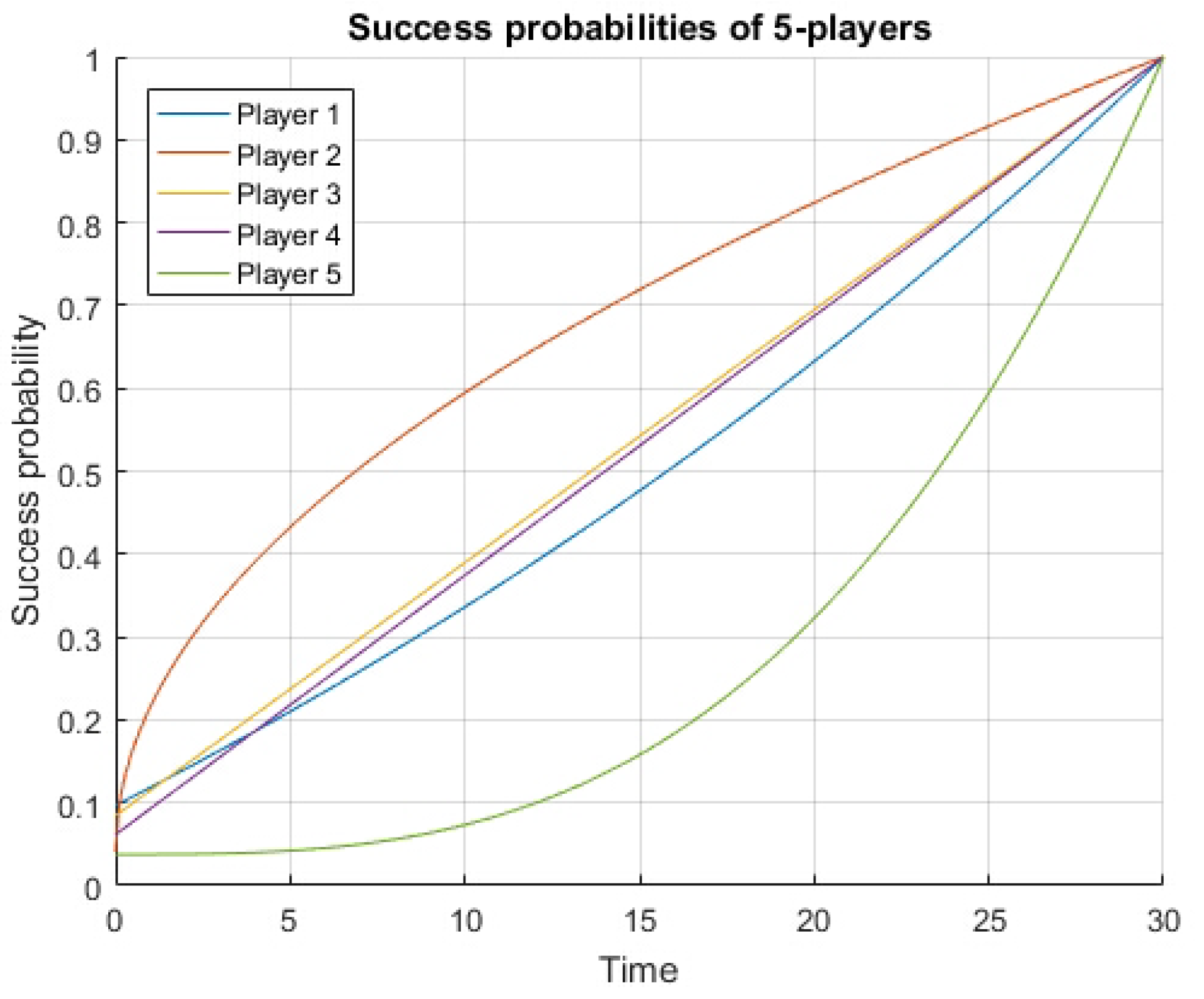
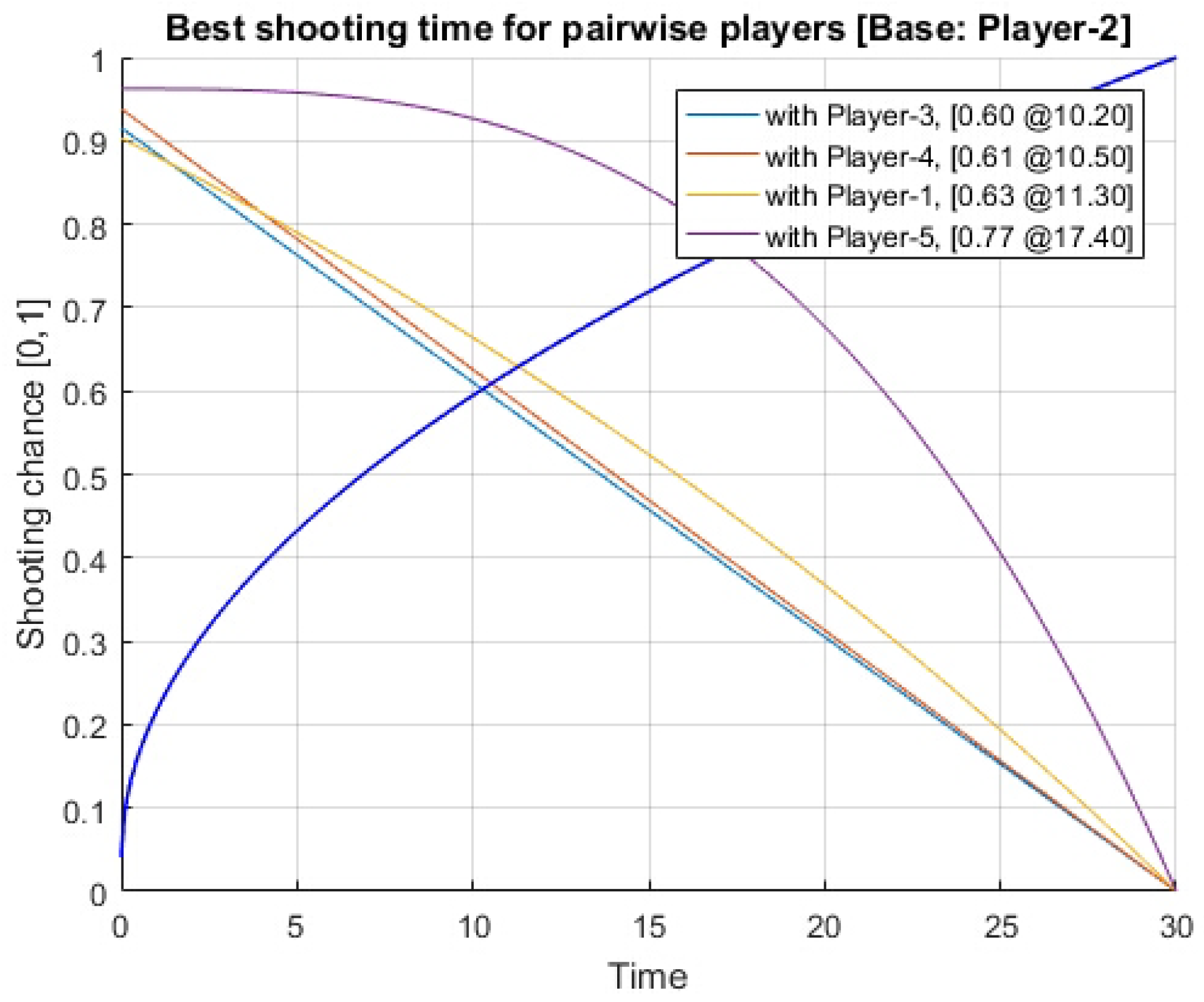
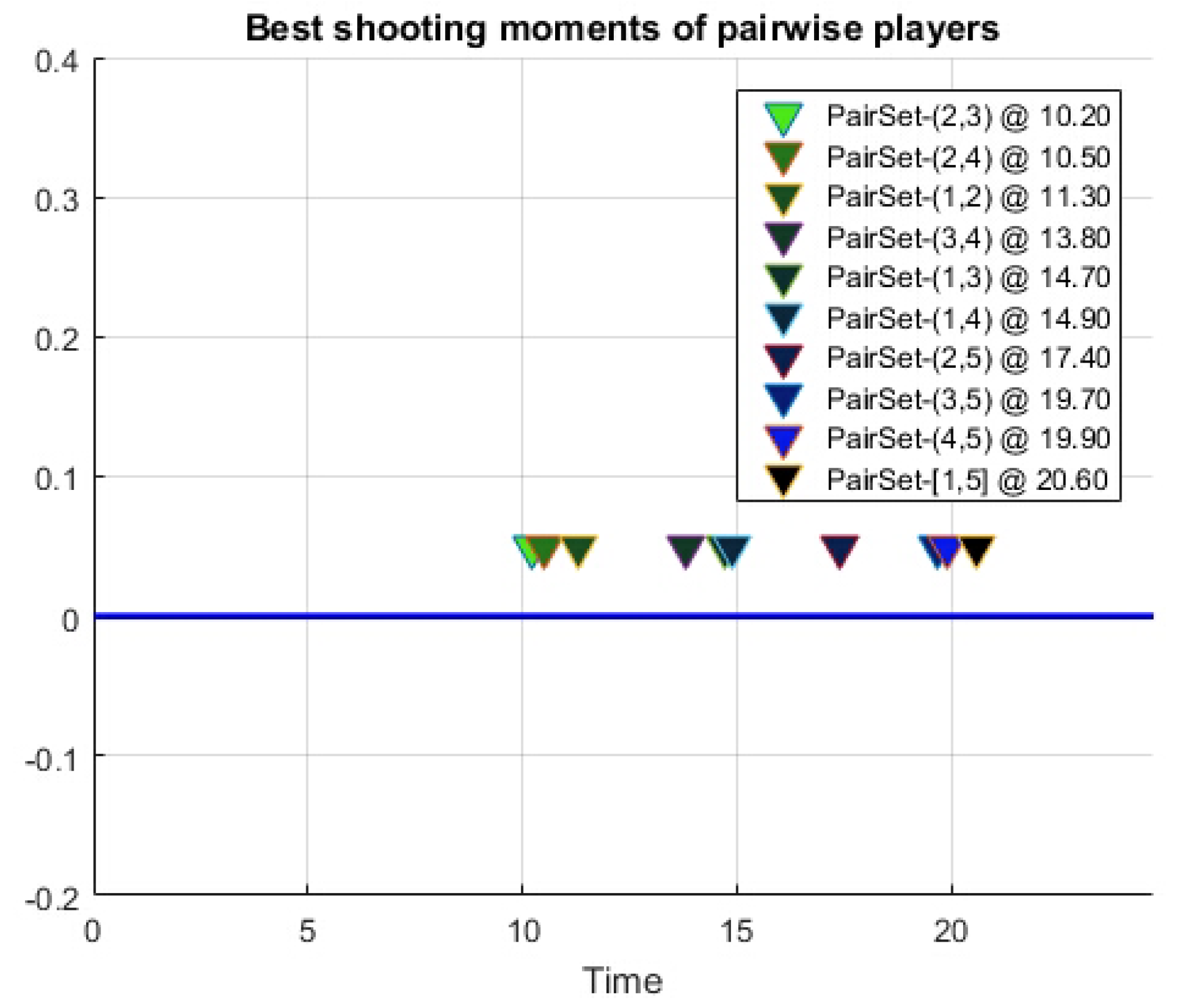
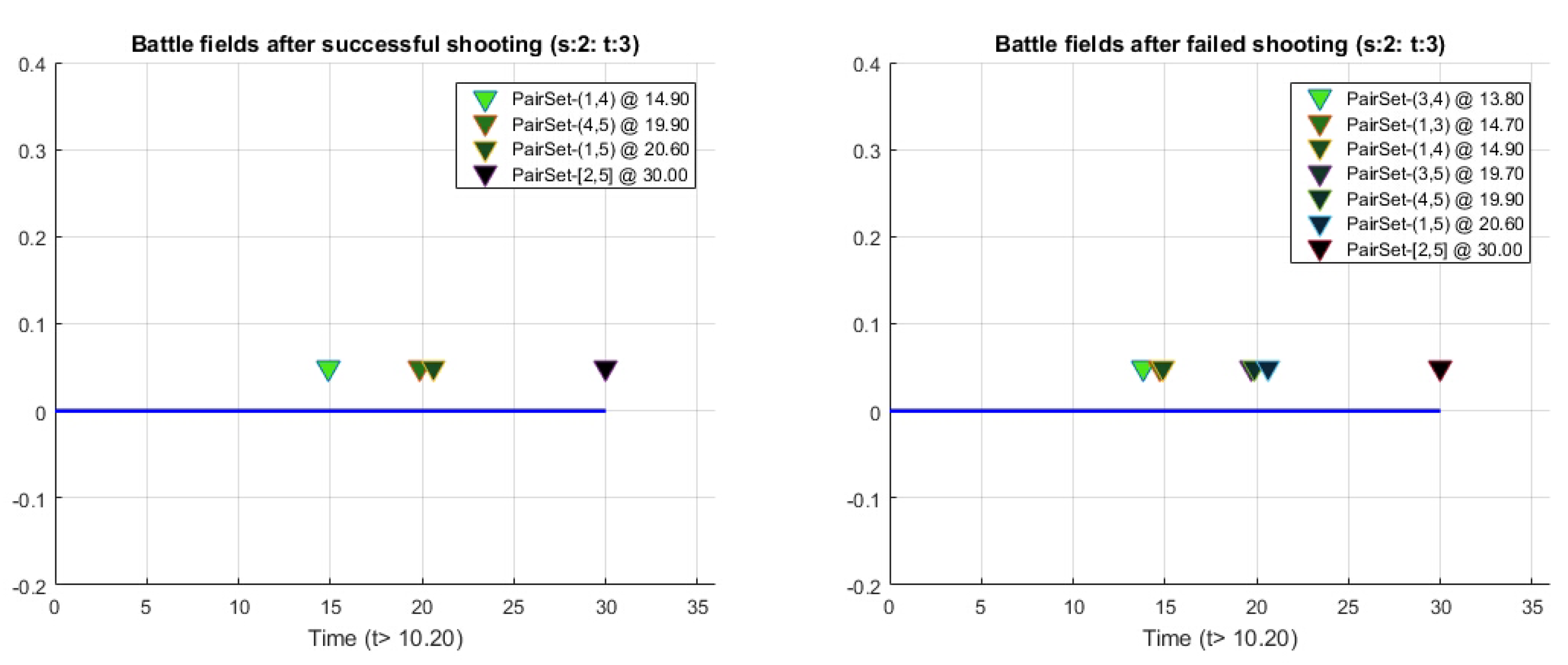
3.3. Numerical Case Practices

Recalling the sample case in the previous section (see Figure 1), let us consider the best shooting strategy of one particular player: player 2. The sequence of battlefields are provided from Equation (42) as follows:

$${\mathit{t}}_{\mathbf{2}}^{\mathbf{0}}=\left\{10.2\le 10.5\le 11.3\le 17.4\right\}$$

(52)

and player 2 is sequentially competing with player 3, player 4, player 1, and player 5 on the first ($m=1$), the second ($m=2$), the third ($m=3$), and the seventh ($m=7$) battlefields. From Equations (43) and (44), the battlefield indicators for each battlefield are as follows:

$${\varrho }_{23}^1=\frac{{\mathcal{P}}_{23}^1}{{\mathcal{P}}_{32}^1}=\frac{0.6}{0.4}=1.5,{\varrho }_{24}^2=\frac{{\mathcal{P}}_{24}^2}{{\mathcal{P}}_{42}^2}=\frac{0.61}{0.37}=1.65,$$

(53)

$${\varrho }_{21}^3=\frac{{\mathcal{P}}_{21}^3}{{\mathcal{P}}_{12}^3}=\frac{0.37}{0.77}=0.55,{\varrho }_{25}^7=\frac{{\mathcal{P}}_{25}^7}{{\mathcal{P}}_{52}^7}=\frac{0.77}{0.82}=0.93.$$

(54)

From (53) and (54), the battlefield and the shooting moment of player 2 are

$$m_i^{*}=3,t_2^{*}=t_{\left\{2,1\right\}}^3$$

(55)

and the opponent player of player 2 (i.e., the target) is player 1. It is noted that this model could easily be extended to the case of multiple shooting chances of a player instead of single chance to shoot. In the same game setup, we could consider that player 2 has two bullets instead of one bullet. From (51), we have the set of the battlefields as follows:

$${\mathit{m}}_2^{*}=\left\{3,7\right\}$$

(56)

and the best shooting times are $t_{\left\{2,1\right\}}^3$ and $t_{\left\{2,5\right\}}^7$, which are equivalent to the third (i.e., $m_2=3$) and seventh (i.e., $m_2=7$) battlefields for player 2. It is noted that all information, including which players are joining, which players are most likely to win, and the best shooting moment of each joined player, is stochastically determined once a battlefield is confirmed. The rest of the analysis is the same as in a basic two-person versatile stochastic duel game [18].

4. Conclusions

A series of antagonistic stochastic duel games was studied and the latest research allows antagonistic multiple player stochastic duel games to be generally expanded. The concept of a battlefield, which is a time sensitive multiple game status, was adapted to simplify a complex game model enough to be analytically solvable. In each battlefield, the actual shooting opportunities are only allowed for pairwise players in the field. This new robust duel game model brings together several studies under the field versatile stochastic duel games. The battlefield indicators not only provide the best shooting moment but also provide the most threatening target player. Both analytical and algorithmic approaches were fully explored to understand the core of an n-person stochastic duel game. A compact closed form of the process was constructed to analyze the best strategies of pairwise players on each battlefield and this analytical form was robustly expanded to the entire game system. The corresponding Matlab source codes are publicly available for users who are interested in implementing this duel game model in their research.

References

1. Konstantinov, R.V.; Polovinkin, E.S. Mathematical simulation of a dynamic game in the enterprise competition problem. Cybern. Syst. Anal. 2004, 40, 720–725. [Google Scholar] [CrossRef]
2. Kam, S.; Wong, S.; Tong, C. The influence of market orientation on new product success. Eur. J. Innov. Manag. 2012, 15, 99–121. [Google Scholar]
3. Kalish, S.; Mahajan, V.; Muller, E. Waterfall and sprinkler new-product strategies in competitive global markets. Int. J. Res. Mark. 1995, 12, 105–119. [Google Scholar] [CrossRef]
4. Azzone, G.; Pozza, I.D. An integrated strategy for launching a new product in the biotech industry. Manag. Decis. 2003, 41, 832–843. [Google Scholar] [CrossRef]
5. Johnson, B.; Laszka, A.; Grossklags, J.; Vasek, M.; Moore, T. Game-theoretic analysis of ddos attacks against bitcoin mining pools. In International Conference on Financial Cryptography and Data Security; Springer: Berlin, Germany, 2014; pp. 72–86. [Google Scholar]
6. Laszka, A.; Johnson, B.; Grossklags, J. When bitcoin mining pools run dry. In International Conference on Financial Cryptography and Data Security; Springer: Berlin, Germany, 2015; pp. 63–77. [Google Scholar]
7. Kim, S.-K.; Yeun, C.Y.; Damiani, E.; Al-Hammadi, Y.; Lo, N.W. Blockchain Adoptation For Automotive Security by Using Systematic Innovation. In Proceedings of the 2019 IEEE Transportation Electrification Conference and Expo, Asia-Pacific (ITEC Asia-Pacific), Seogwipo, Korea, 8–10 May 2019; pp. 1–4. [Google Scholar]
8. Kim, S.-K. Enhanced IoV Security Network by Using Blockchain Governance Game. Mathematics 2021, 9, 109. [Google Scholar] [CrossRef]
9. Polak, B. Discussion of Duel. Open Yale Courses. 2008. Available online: http://oyc.yale.edu/economics/econ-159/lecture-16 (accessed on 1 May 2019).
10. Moschini, G. Nash equilibrium in strictly competitive games: Live play in soccer. Econ. Lett. 2004, 85, 365–371. [Google Scholar] [CrossRef]
11. Radzik, T. Games of Timing Related to Distribution of Resources. J. Optim. Theory Appl. 1988, 58, 443–471. [Google Scholar] [CrossRef]
12. Radizik, T. Silent Mixed Duels. Optimization 1989, 20, 553–556. [Google Scholar] [CrossRef]
13. Lang, J.P.; Kimeldorf, G. Silent Duels with Non Discrete Firing. SIAM J. Appl. Math. 1976, 31, 9–110. [Google Scholar] [CrossRef]
14. Schwalbe, U.; Walker, P. Zermelo and the Early History of Game Theory. Games Econ. Behav. 2001, 34, 123–137. [Google Scholar] [CrossRef] [Green Version]
15. Kingston, C.G.; Wright, R.E. The deadliest of games: The institution of dueling. South. Econ. J. 2010, 76, 1094–1106. [Google Scholar] [CrossRef] [Green Version]
16. Dshalalow, J.H.; White, R. On Reliability of Stochastic Networks. Neural Parallel Sci. Comput. 2013, 21, 141–160. [Google Scholar]
17. Dshalalow, J.H.; Iwezulu, K.; White, R.T. Discrete Operational Calculus in Delayed Stochastic Games. Neural Parallel Sci. Comput. 2016, 24, 55–64. [Google Scholar]
18. Kim, S.-K. A Versatile Stochastic Duel Game. Mathematics 2020, 8, 678. [Google Scholar] [CrossRef]
19. Kim, S.-K. Antagonistic One-To-N Stochastic Duel Game. Mathematics 2020, 8, 1114. [Google Scholar] [CrossRef]
Figure 1. Success probabilities for a five-person duel game.
Mathematics 09 00825 g001
Figure 2. Best pairwise shots for player 2 in multiple battlefields.
Mathematics 09 00825 g002
Figure 3. The shooting order of a five-person duel game.
Mathematics 09 00825 g003
Figure 4. The battlefield status after shooting on the first battlefield.
Mathematics 09 00825 g004
Publisher’s Note: MDPI stays neutral with regard to jurisdictional claims in published maps and institutional affiliations.