Article

A Method of Riemann–Hilbert Problem for Zhang’s Conjecture 1 in a Ferromagnetic 3D Ising Model: Trivialization of Topological Structure

1
Department of Computer and System Analysis, College of Humanities and Sciences, Nihon University, Sakurajosui 3-25-40, Setagaya-ku, Tokyo 156-8550, Japan
2
Shenyang National Laboratory for Materials Science, Institute of Metal Research, Chinese Academy of Sciences, 72 Wenhua Road, Shenyang 110016, China
*
Author to whom correspondence should be addressed.
Mathematics 2021, 9(7), 776; https://doi.org/10.3390/math9070776
Submission received: 8 February 2021 / Revised: 26 March 2021 / Accepted: 28 March 2021 / Published: 2 April 2021

Abstract

:
A method of the Riemann–Hilbert problem is applied for Zhang’s conjecture 1 proposed in Philo. Mag. 87 (2007) 5309 for a ferromagnetic three-dimensional (3D) Ising model in the zero external field and the solution to the Zhang’s conjecture 1 is constructed by use of the monoidal transform. At first, the knot structure of the ferromagnetic 3D Ising model in the zero external field is determined and the non-local behavior of the ferromagnetic 3D Ising model can be described by the non-trivial knot structure. A representation from the knot space to the Clifford algebra of exponential type is constructed, and the partition function of the ferromagnetic 3D Ising model in the zero external field can be obtained by this representation (Theorem I). After a realization of the knots on a Riemann surface of hyperelliptic type, the monodromy representation is realized from the representation. The Riemann–Hilbert problem is formulated and the solution is obtained (Theorem II). Finally, the monoidal transformation is introduced for the solution and the trivialization of the representation is constructed (Theorem III). By this, we can obtain the desired solution to the Zhang’s conjecture 1 (Main Theorem). The present work not only proves the Zhang’s conjecture 1, but also shows that the 3D Ising model is a good platform for studying in deep the mathematical structure of a physical many-body interacting spin system and the connections between algebra, topology, and geometry.

1. Introduction

The study on the Ising model has attracted intensive interest since the 1920s [1], which not only applies to interpret phase transitions and critical phenomena in different fields, but also provides fundamental understanding on interactions and dimensionality in nature. Onsager derived the exact solution of a two-dimensional (2D) Ising model in the zero external field, in which no non-trivial topological structures exist [2]. There had been no rigorous results on the solution of a three-dimensional (3D) Ising model in the zero external field, even for a simplest case with all interactions ferromagnetic. On the observation of the formula of the partition functions, the second author (ZDZ) made an observation that non-trivial topological structures exist in the ferromagnetic 3D Ising lattices in the zero external field for any positive inverse temperature [3,4]. This observation consists with the point view of Newell and Montroll [5], who pointed out that for the 3D Ising model in the zero external field, one encounters polygons with knots. Moreover, the second author conjectured that the non-trivial knot/link structures of the ferromagnetic 3D Ising model in the zero external field can be trivialized in higher dimensional space and the ferromagnetic 3D Ising model can be realized as the free statistic model on the (3+1)-dimensional space-time with topological/geometrical phases on eigenvectors [3,4]. The algebraic part of the quaternion approach used in [3] was reformulated in terms of the quaternionic sequence of Jordan algebras to look at the geometrical aspects of simple orthorhombic Ising lattices [6], and fractals and chaos related to these 3D Ising lattices were investigated [7]. Zhang, Suzuki, and March developed a Clifford algebra approach for the ferromagnetic 3D Ising model in the zero external field, and proved four Theorems (Trace Invariance Theorem, Linearization Theorem, Local Transformation Theorem, and Commutation Theorem) [8]. It proves rigorously the Zhang’s two conjectures and verifies that the exact solution based on the Zhang’s conjectures [3] is correct. The explicit expressions for the partition function, the specific heat, the spontaneous magnetization, the spin correlation, and the susceptibility of the ferromagnetic 3D Ising model in the zero external field can be found in [3]. The critical exponents of the ferromagnetic 3D Ising model are determined to be α = 0, β = 3/8, γ = 5/4, δ = 13/3, η = 1/8, and ν = 2/3, satisfying the scaling laws [3]. In a recent work [9], the lower bound of the computational complexity of a spin-glass 3D Ising model was determined, which was based on deep understanding on the mathematical structure of the Ising models on 3D lattices. More recently, the exact solution of ferromagnetic/antiferromagnetic 2D Ising model with a transverse field is derived by equivalence between the ferromagnetic/antiferromagnetic 2D Ising model with a transverse field and the ferromagnetic/antiferromagnetic 3D Ising model in the zero external field [10].
Before processing the present work, we would like to compare the exact solution of the ferromagnetic 3D Ising model with other results in the literature. Since publication of Zhang’s conjectured exact solution [3], there has been a series of criticisms from Wu, McCoy, Fisher and Chayes [11,12], Perk [13,14,15], and Fisher and Perk [16]. The main contents of their comments [11,12,13,14,15,16] are summarized briefly as follows: (1) The exact high-temperature series is not reproduced, which has been proved rigorously to be convergence at temperature greater than any positive number. (2) The exact low-temperature series is not reproduced, even in the first term. (3) The Jordan–Wigner transform used in the very beginning of Zhang’s original paper [3] is invalid. (4) The critical exponents α = 0 and γ = 5/4 for the solution to the 3D Ising model differ from perturbative, nonperturbative, and even experimental results, all of which are consistent with each other [16], with a special emphasis of new results of El-Showk et al. [17] using convex optimization of the c-parameter within the conformal bootstrap approach to the four-point correlation functions. We do not want to repeat Zhang’s detail responses published already [3,4,8,18,19]. Just mention also briefly: The error for the Jordan–Wigner transform in Zhang’s original paper [3] is not a problem, which has been corrected in [4,8], and Zhang’s two conjectures can start from the corrected formula with the non-trivial topological structure. The topological effects indeed exist as clearly seen from the corrected Jordan–Wigner transform [4,8,13,20], which were indicated clearly in [5] and proven rigorously in [21]. The so-called exact and rigorous approaches of 1960s and later [22,23,24,25,26,27] for the 3D Ising model are rigorous only for β = 1/(kBT) > 0, not for β = 0. The so-called exact low-temperature expansion is evidently divergent, which indicates that this expansion approach is not exact, not only for its high-order terms, but also for the first term, as the approach itself is questionable. The Lee–Yang Theorem for phase transitions offers a possibility of a phase transition at infinite temperature in the Ising models [28,29], which provides a possibility of multi-valued functions for high-temperature expansions. Note that the convergences of βf and f are different at/near infinite temperature. The approximation methods (including perturbative, nonperturbative) and computer simulations (including Monte Carlo) do not take into account the contribution of the non-trivial topological structure of the 3D Ising model to the physical properties. Missing the global effect is the main reason that all these approximation methods consist with each other, but are incorrect due to the existence of systematical errors, no matter how high precision they achieve. The systematical errors of these approximation techniques are related directly to the physical conceptions/pictures at the first beginning and the neglects of important non-locality factors during procedures. As pointed out in [30] that these estimates in [17] were obtained based on certain hypotheses (e.g., the existence of a sharp kink) and that if these hypotheses are not used, then the conformal bootstrap analysis appears to be consistent with the values η = 1/8 and ν = 2/3, obtained by Grouping of Feynman Diagrams, which are consistent with the Zhang’s solutions obtained in [3]. Furthermore, Zhang’s results agree with some experimental results, which are carefully performed with high accuracy (see in [31], for instance). After its publication [3], Zhang’s conjectured solution has received supports from several groups, for instance, March and his co-workers [32,33,34,35,36], Ławrynowicz and some mathematicians [6,7,37,38], Kaupuzs and his colleagues [30,39,40], and others [41,42,43,44,45,46,47,48,49,50,51,52,53]. In [8], Zhang-Suzuki-March rigorously proved four Theorems, which verifies the correctness of the Zhang’s conjectured solution [3]. The correct way to judge the correctness of an exact solution is to check whether there is anything wrong in the deriving process of proofs of Theorems, not to judge it by the approximant results. After the publication of Zhang-Suzuki-March’s work [8], up to date, no further criticisms have been published. It was suggested that the approximation techniques can be utilized to obtain the non-locality part of the partition function (as well as the thermodynamic physical properties) by extracting the approximation values from the exact solution [54,55].
Although the Clifford algebra approach developed in [8] has already verifies the correctness of the exact solution based on the Zhang’s two conjectures [3], it is still of great interest to prove the two conjectures from other mathematical aspects. In this way, the 3D Ising model and its exact solution would serve as a platform for investigating the connections between algebra, geometry, and topology, which are associated with the mathematical structure of the 3D Ising model. In this work, we will develop a method of Riemann-Hilbert problem for Zhang’s conjecture 1, regarding the trivialization of the topological structure. The method of Riemann–Hilbert problem for Zhang’s conjecture 2, regarding to the generation of topological phases, is in progress. In Section 2, the Hamiltonian and partition function of the ferromagnetic 3D Ising model in the zero external field are represented, and the Zhang’s conjecture 1 is introduced with mathematical aspects. In Section 3, the Clifford algebra of the ferromagnetic 3D Ising model and its Knot/Clifford (K/C) algebra are constructed. In Section 4, the knot structure of the ferromagnetic 3D Ising model in the zero external field is investigated, and the partition function of the 3D Ising model can be generated by construction of the K/C-knots with the normal lattice knot γ, two types of basic knots (circles and braids), and their crossings. In Section 5, the knot/link structure is realized on a hyperelliptic Riemann surface, by the complex analysis. In Section 6, the method of the Riemann–Hilbert problem is applied for the representation. In Section 7, monoidal transforms are applied to give the desired trivialization of knot structures. In Section 8, the construction of solution to the Zhang’s conjecture 1 is given, based on the procedures in the previous sections, which proves the Main Theorem, namely, that Zhang’s conjecture 1 has been proven. In Section 9, the conclusion is given. The details for proofs of Theorems II and III are represented in Appendix A and Appendix B, respectively.

2. 3D Ising Model and Zhang’s Conjectures

We recall some basic facts on the ferromagnetic 3D Ising model in the zero external field and represent its description by Clifford algebra.

2.1. Hamiltonian and Partition Function of 3D Ising Model

We consider the orthorhombic lattice in the 3D Euclidean space [3,4]. Either up-spin or down-spin is located at each lattice point. The Hamiltonian of this statistical model is given as
H = H1 + H2 + H3
{ H 1 = J τ = 1 n ρ = 1 m δ = 1 l s ρ , δ ( τ ) s ρ , δ ( τ + 1 ) H 2 = J τ = 1 n ρ = 1 m δ = 1 l s ρ , δ ( τ ) s ρ + 1 , δ ( τ ) H 3 = J τ = 1 n ρ = 1 m δ = 1 l s ρ , δ ( τ ) s ρ , δ + 1 ( τ )
Here, only the nearest neighboring interaction between spins at each lattice point is considered. J, J′ and J″ are ferromagnetic interaction constants along three crystallographical axes of the lattice, respectively.
The partition function Z of the ferromagnetic 3D Ising model in the zero external field can be given as follows [3,4,8]:
Z = ( 2 sinh 2 K ) m n l 2 t r a c e ( V 3 V 2 V 1 ) m ( 2 sinh 2 K ) m n l 2 i = 1 2 n l λ i m
V 3 = j = 1 n l exp { i K Γ 2 j [ k = j + 1 j + n 1 i Γ 2 k 1 Γ 2 k ] Γ 2 j + 2 n 1 } = j = 1 n l exp { i K s j s j + n } ;
V 2 = j = 1 n l exp { i K Γ 2 j Γ 2 j + 1 } = j = 1 n l exp { i K s j s j + 1 } ;
V 1 = j = 1 n l exp { i K * Γ 2 j 1 Γ 2 j } = j = 1 n l exp ( K * C j ) .
Here, we introduce variables K = J / ( k B T ) , K = J / ( k B T ) and K = J / ( k B T ) instead of J, J′ and J″. K* is defined by e 2 K tanh K * [2,3,4,20,56]. We define the matrices C j and s j as follows: C j = I I I C I I and s j = I I I s I I . Note that although only the nearest neighboring interaction between spins at each lattice point is considered in the Hamiltonian, the expressions of higher degree than quadratic in Γ-matrices (i.e., non-local terms like the log of V3) appear in the partition function, which represent the existence of a long-range many-body entanglement between spins in the ferromagnetic 3D Ising model, because of the nature of three dimensions.

2.2. Zhang’s Conjecture 1

Here, we discuss the main problem on a ferromagnetic 3D Ising model in the zero external field and state the Zhang’s conjecture 1. Although the ferromagnetic 3D Ising model we studied has the nearest neighboring interaction only, the nature of three dimensions results in two different behaviors for the interactions: (i) C j or s j s j + 1 represents the nearest interaction along the first or second dimension, and (ii) s j s j + n represents the nearest interaction along the third dimension, which consists of the non-local behavior, namely, a kind of long-range many-body entanglement. The interaction C j or s j s j + 1 can be described by use of the Lie group/algebra (so-called Gaussian type). The main concern is s j s j + n , which leads to our main problem of trivialization for the non-trivial knot structure. Zhang has discussed this problem in terms of topology [4], namely, the knot theory [57,58]. Topologically, there are two choices for smoothing a given crossing (×), and thus there are 2N states of a diagram with N crossings [57,58]. The bracket state summation is an analog of a partition function in discrete statistical mechanics, which can be used to express the partition function for the Potts model for appropriate choices of commuting algebraic variables [57,58]. This means that not only the local spin alignments but also the crossings of knots contribute to the partition function Z of the 3D Ising model in the zero external field. The contribution to the partition function Z by knots also reflects the entropy cost of tying knots, as the partition function Z is related with the free energy F, the internal energy U, and the entropy S.
In this paper, we introduce the knot structure which is called “Knot/Clifford (K/C) knot” and associate the knot for the partition function. We can have the representation from the K/C knot to Clifford algebra, and describe the topological structure of the partition function of the ferromagnetic 3D Ising model in the zero external field, which might give the answer of the problem by making the trivialization of the given (non-trivial) knot. The trivialized knots constitute with the knot of trivial type only.
Consider the 3D lattice Z3 and take a knot γ which is constructed by the horizontal line and vertical joint line with vertex {Pj}, which is denoted by γ = {Pj}, as illustrated below in Figure 1, for example.
Generators of the transfer matrices V1, V2, and V3 are associated to some points in γ, which are denoted by X = {Vi(j)}. Then, we have a data (γ, X) which is called Knot/Clifford (K/C) data, Z γ . The Zhang’s conjecture 1 can be stated in the following manner:
  • For a given Z γ , can we make a trivialization Z ˜ γ ˜ ?
  • More exactly, we can state the Zhang’s conjecture 1 as:
Can we find a four-dimensional manifold M ˜ 4 , and a K/C data { γ ˜ , X ˜ } on M ˜ , where γ ˜ is usually a nontrivial knot (however, it can also be a trivial one for simple cases) and X ˜ = { Γ ˜ j } , Γ ˜ j is a member of generators satisfying the following condition. We can find a trivialization mapping, F : M ˜ × K / C ( M ˜ ) Z 3 × K / C ( Z 3 ) , satisfying F ( Z ˜ γ ˜ ) = Z γ . Here, we have put Z ˜ γ ˜ = { γ ˜ , X ˜ } .

2.3. Steps to Prove Zhang’s Conjecture 1 on Trivialization

In this paper, we shall give a positive answer to the Zhang’s conjecture 1 in the following steps:
(1)
The Clifford algebra C l ( I 3 D ) is extended to the K/C algebra which has the original Clifford algebra and its conjugate algebra C l ( I 3 D ) ¯ as subalgebras (Section 3).
(2)
Z γ is extended to the K/C algebra which is denoted by σ ( Z γ , Z ¯ γ ) . Therefore, we have a knot carrying the elements in K/C algebra for the partition function (Section 4).
(3)
After the realization of the knot on a Riemann surface (Section 5), we formulate the Riemann–Hilbert problem for the representation and obtain the solution (Section 6).
(4)
Applying the monoidal transformation to the solution in (3), we construct the desired trivialization in K/C algebra (Section 7).

3. Clifford Algebra of the Ferromagnetic 3D Ising Model and Its K/C Algebra

In this section, we state the generation of Clifford algebra of the ferromagnetic 3D Ising model in the zero external field by the basic construction and then give its extension which is called a K/C algebra.

3.1. Clifford Algebra of the Ferromagnetic 3D Ising Model

We give the basic construction of Clifford algebra and list up the generators.
Let Cl(2N−1, C) be the Clifford algebra with the generators Aj (j = 1,2,…, 2N−1):
A k A j + A j A k = 2 δ k j 1
Then, putting A ˜ j = σ 1 A j = [ 0 A j A j 0 ] (j = 1,2,…,2N−1),
A ˜ 2 N = σ 2 E = [ 0 i E i E 0 ]   ( i 2   =   1 ) ,   A ˜ 2 N + 1 = σ 3 E = [ E 0 0 E ] ,  
where σ i ( i = 1 , 2 , 3 ) . We can obtain the Clifford algebra Cl(2N+1,C) with the generators A ˜ j Aj (j = 1,2,…,2N+1).
A ˜ k A ˜ j + A ˜ j A ˜ k = 2 δ k j I
Repeating the basic construction successively, we can obtain general Clifford algebra:
Following the notation due to Onsager-Kaufman-Zhang [2,3,4,8,56], we choose the notation s = [ 0 1 1 0 ] (= iσ2), s = [ 1 0 0 1 ] (= σ3), C = [ 0 1 1 0 ] (= σ1). Following the generation process of Clifford algebra based on C, we obtain the generation
C l ( 3 , C ) :   C , s , s
C l ( 5 , C ) :   C C , C s , C s , s 1 , s 1
C l ( 7 , C ) :   C C C , C C s , C C s , C s 1 , C s 1 s 1 1 , s 1 1
……
C l ( 2 N 1 , C ) :   C C C C ( 2 N 1   times   C )
C C C C s    ( 2 N 2   times   C )
……
C C C s 1 1    ( r   times   C )
……
C s 1 1 ( 1   times   C )
s 1 1 ( 0   times   C )
s 1 1   ( 0   times   C )
Therefore, we can introduce the following generators of Clifford algebra of the 3D Ising model:
Γ 2 k 1 = C C C s 1 1    ( k 1   times   C )
Γ 2 k = C C C ( i s ) 1 1    ( k 1   times   C )

3.2. K/C Algebra Associated to the Knot Structure

We introduce the K/C algebra which is an extension of Clifford algebra of the ferromagnetic 3D Ising model. We put the generators of the Clifford algebra and its conjugate elements:
Γ i = C C s ( i ) 1 1
Γ ¯ i = C ¯ C ¯ s ¯ ( i ) 1 ¯ 1 ¯
where
s ( i ) = { s 1 s ( i = 2 j 1 ) ( i = 2 j ) ,   s ¯ ( i ) = s ( i ) ,
In order to obtain the commutation relations { Γ i , Γ ¯ j } , we introduce the following algebra with the product table which is called knot-algebra (see Table 1).
The product is defined by a b . For example, 1 ¯ 1 = 1 ¯ , 1 ¯ C = C ¯ , etc.
We can obtain the following proposition.
Proposition: 
(1)
Knot/Clifford algebra is an associative algebra.
(2)
We have Γ i Γ j = Γ i Γ ¯ j , Γ ¯ i Γ j = Γ ¯ i Γ ¯ j . Here, we have calculated the product including s , s as the usual matrix calculus. It implies that the first element determines the sequence to be Γ-sequence or Γ ¯ sequence.
In the following we call Γ-sequence positive sequence, Γ ¯ -sequence negative sequence, respectively.
The K/C algebra has the following commutation relation: Γ i Γ j + Γ j Γ i = 2 δ i j I ; Γ i Γ ¯ j + Γ ¯ j Γ i = 2 δ i j I ; Γ ¯ i Γ j + Γ j Γ ¯ i = 2 δ i j I ; Γ ¯ i Γ ¯ j + Γ ¯ j Γ ¯ i = 2 δ i j I .
It is seen that the K/C algebra has subalgebras which are real Clifford algebra and its conjugate algebra, and they are conjugate each other.

4. Knot Structure of the Ferromagnetic 3D Ising Model

In this section, we introduce a special class of knots, which are called knots of the ferromagnetic 3D Ising model in the zero external field, by use of the product structure of Γ-factors. Then, the representation from the K/C algebra of 3D Ising type to the knots of 3D Ising type can be found.
The topological structures of the ferromagnetic 3D Ising model in the zero external field are constructed by two parts of contributions. First, there exist normal (either trivial or nontrivial) knots γ (or links), which are generated by lattice points. Second, the Pauli matrices themselves may be treated as crossings [57,58], which also contribute the fine structure of the topology. The latter case is the main concern of this paper, as the non-linear terms in the partition function contribute the non-trivial topological structure of the ferromagnetic 3D Ising model in the zero external field.

4.1. Knots with Clifford Algebra Data

In this paper, when we say a knot, it has always Clifford algebra data. We choose a knot γ which is generated by lattice points {P1, …, Pn}. Namely, γ = P1, …, Pn. Choosing elements X 1 , X n , X 1 , X n C l ( I 3 D ) , and making their conjugates X ¯ 1 , X ¯ n . ( X i , X ¯ i ) is associated to γ at Pi. The sequence is denoted by
γ ( X , X ¯ ) = ( P 1 ( X 1 , X ¯ 1 ) ) ( P n ( X n , X ¯ n ) )

4.2. Association of Circle/Interval to Γ-Factors

We choose an element Γ C l ( I 3 D ) and associate a circle (or interval) to Γ.
Γ k = C C C s ( k ) 1 1
We take its conjugate element Γ ¯ k ¯ C l ( I 3 D ) ¯ and associate a dotted circle (or dotted interval):
Γ ¯ k = C ¯ C ¯ C ¯ s ¯ ( k ) 1 ¯ 1 ¯

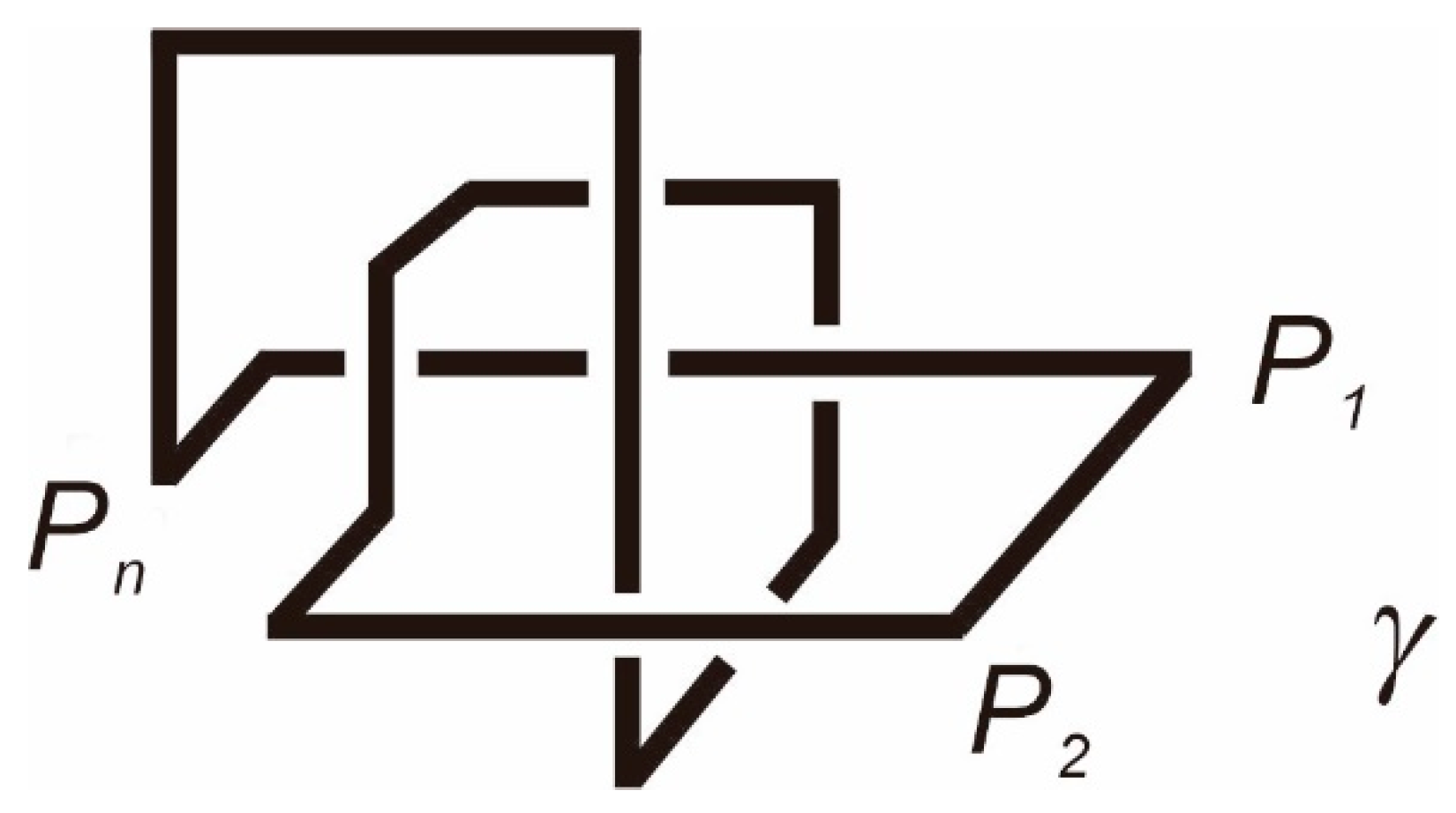
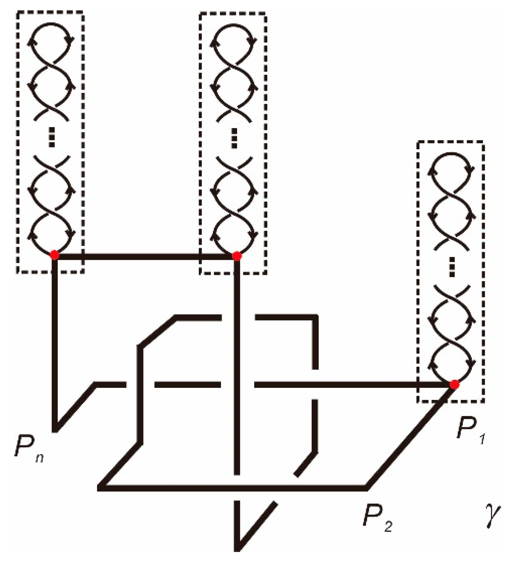
4.3. Generation of Knots of Ferromagnetic 3D Ising Model for Partition Functions

We treat the knot structure of the partition function of the ferromagnetic 3D Ising model in the zero external field as follows. There exist two types of basic forms: the elements i Γ i Γ j (and i Γ ¯ i Γ ¯ j ) can be represented as a circle (or an interval), while the element i Γ i Γ ¯ j or i Γ ¯ i Γ j can be represented by the following knot called basic form of type I (see Figure 2).
The detailed construction of this knot structure from Pauli matrices in the transfer matrices V1 and V2 are omitted for simplicity. The elements i k ( Γ i 1 Γ j 1 ) ( Γ i k Γ j k ) (and i k + 1 Γ i ( Γ i 1 Γ j 1 Γ i k Γ j k ) Γ j ) (with j = 1,2,…,nl; k = 2n) together with their conjugate elements are called basic form of type II (see Figure 3), which can be represented as a braid with many crosses (k = 2n).
Indeed, each factor of i Γ 2 k 1 Γ 2 k in the internal factors of the transfer matrices V3 is equal to the Pauli matrix σ k z [13], contributing a crossing topologically [57,58]. Therefore, each term of exponential elements in the transfer matrices V1 and V2 contributes a circle to the knot structure, while each term of exponential elements in V3 contributes a braid. There is also a type which is defined by the product of exponential elements generated by the basic types above. The circles in V1 and V2 can be adjoined together with the lattice points of the normal knots γ, while the braids in V3 can be connected as the product type of knots. As an example, the following figure (Figure 4) just shows three of the braids in V3 connecting to the lattice points of the knot γ, while it does not show the circles of V1 and V2 for simplicity.
Note that the knot structure of the ferromagnetic 3D Ising model in the zero external field is much more complicated than what we illustrated in the above figure. The other end of these braids should be connected to other lattice points in accordance with the expression for the partition function. Adjoining the braids for different j in V3 forms new crosses, making the topological structure much more complicated. We can introduce a concept of confluency of knots and discuss the generation of K/C knots by use of successive confluence operations, to obtain the K/C knots of the generators Vi (i = 1,2,3) of the partition functions of the ferromagnetic 3D Ising model in the zero external field. Nevertheless, the process for trivialization of the above topological structure can be employed directly to trivialize the more complicated one, as the concept, the principle, the role, and the process are kept the same.
By these observations, we see the following theorem.
Theorem I.
The partition function of the ferromagnetic 3D Ising model in the zero external field can be generated by construction of the K/C-knots with the normal lattice knot γ, two types of basic knots (circles and braids), and their crossings. The transfer matrices V1 and V2 contribute the trivial parts to the topological structure of the ferromagnetic 3D Ising model in the zero external field, while the transfer matrices V3 contribute the non-trivial knots to the system.

5. Realization of Knots on a Riemann Surface

In this section, the knot/link structure is realized on a hyperelliptic Riemann surface. This is the first step of the realization of knot/link structure by the complex analysis.

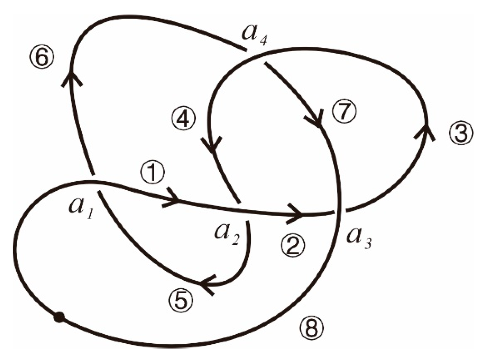
5.1. Realization of Knots

We choose a knot ξ, which is expressed as ξ = α 1 α 2 α 2 n . Assume that ξ is a positive sequence, and that α 1 = a 1 + . The intersection points are denoted as a1, a2, ……, an. We prepare two copies of complex projective space P1. A 2-covering Riemann surface Mg is made by use of cut-segments:
In the case where n is even (n = 2m), one has Figure 5.
In the case where n is odd (n = 2m + 1), one has Figure 6.
In a well-known manner, make a Riemann surface. We demonstrate in Figure 7 the construction of the Riemann surface z : in this case, we make the cut along (0∞) and glue in the figure. As for a general case, the construction is performed in a completely analogues manner.

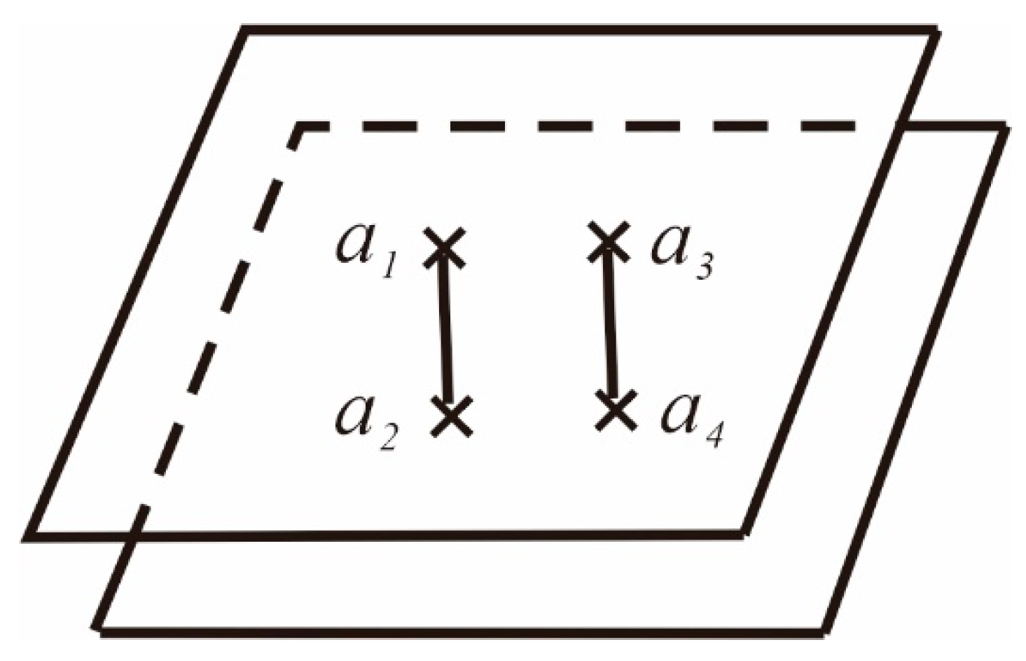
5.2. Realization of Knots on a Four-dimensional Manifold

In order to make clear the role of monoidal transform, we realize the base Riemann surface Mg in P × C as a covering space over P1 (Figure 8). Then, we assume that the knot has a singularity of normal crossing.

5.3. Realization on a Riemann Surface

For the realization of knots on the Riemann surface, we choose a knot ξ with intersection points { a 1 , , a n } . At first, we make a small circle C ε ( j ) at each point aj: C ε ( j ) = { | z a j | = ε } . Assume that C ε ( j ) C ε ( k ) = ϕ ( j k )
(1)
For each aj, we take a ˜ j + , a ˜ j on C ε ( j ) corresponding a j + , a j , respectively.
(2)
Starting from a 1 + , we take a ˜ 1 + on the upper surface.
(3)
The next element is denoted by αk. When α k = a k + , we take a ˜ k + and joint them without cut segment (Figure 9).
When α k = a k , we take a ˜ k on the lower surface and joint them crossing the cut-segment (Figure 10).
(4)
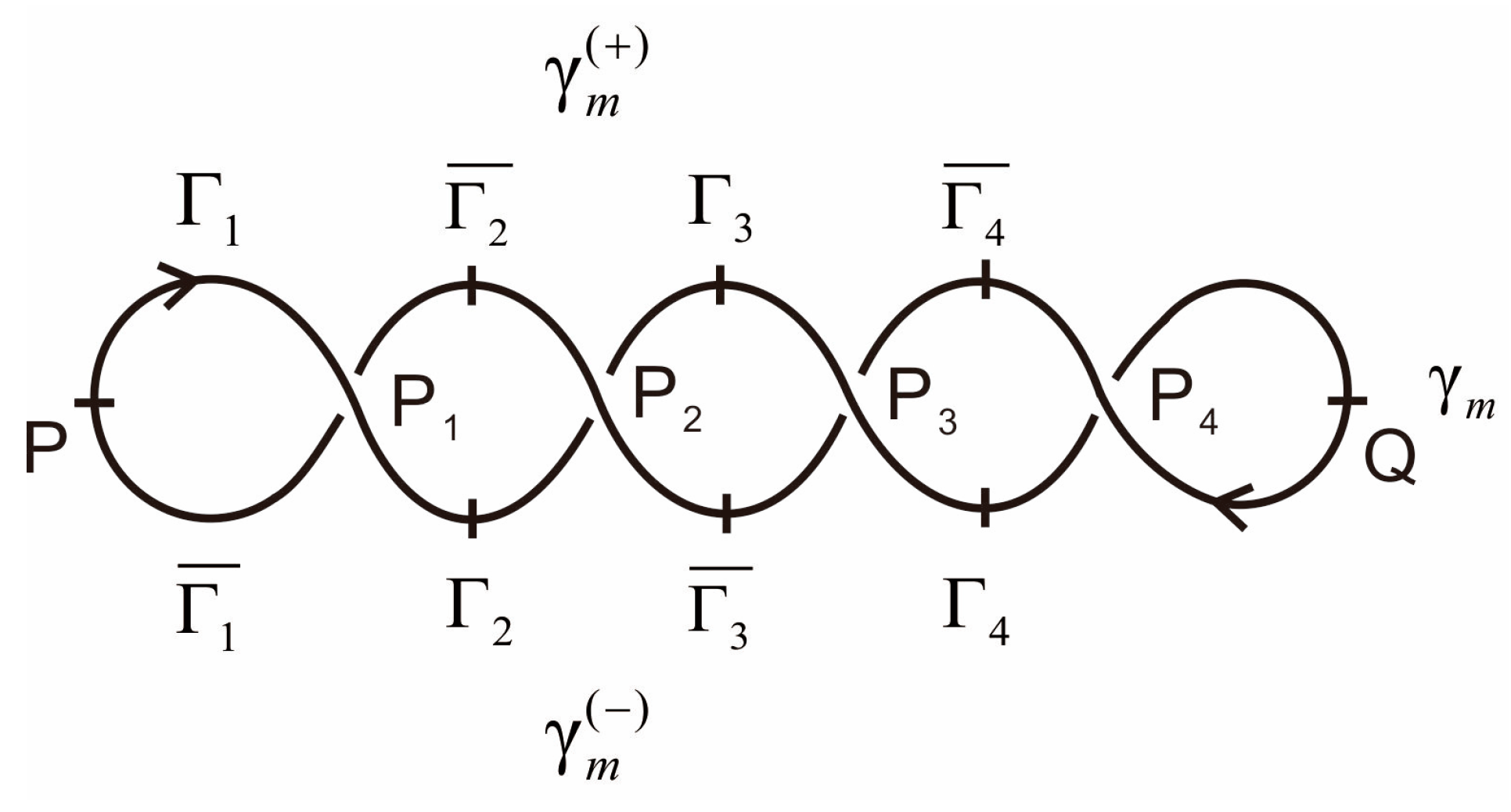
Repeating this process, we obtain a closed curve which is located very near to the original knot curve.
Remark 1.
Here, we have to pay attention to check whether entanglement appears or not. We will not be concerned with this problem. This is because when the entanglement points appear, we extend the knot and associate the trivial matrix and solve our problem.
Example. 
We choose a knot sequence in Figure 11: α = a 1 + a 2 + a 3 a 4 + a 2 a 1 a 4 a 3 + .
We prepare two sheets of P1 and make cuts between a 1 a 2 ¯ , a 3 a 4 ¯ , and make a hyper-elliptic curve. Making small circles at a 1 , a 2 , a 3 , a 4 , and following the generation scheme in Figure 12, we can obtain the realization of the knot in Figure 11 on the Riemann surface.
We can prove the following Proposition.
Proposition. 
From the representation   ρ 0 : K / C ( I 3 D ) e x p ( C l ( I 3 D ) ) , there exists a representation
ρ ˜ 0 : π 1 ( R g { a 1 a N } ) C l ( I 3 D ) e x p ( C l ( I 3 D ) ) ,  
such that the following commutative relations hold:
Mathematics 09 00776 i001

6. Method of Riemann–Hilbert Problem for 3D Ising Model

In this section, the method of the Riemann–Hilbert problem is applied for our representation. At first, let us recall the Riemann–Hilbert problem.

6.1. Riemann-Hilbert Problem

As for a function f on a compact Riemann surface Rg which has a regular singularity at a1, a2, …, aM. The function has the following form:
f ( z ) = ( z a j ) β ( c o ( j ) + c 1 ( j ) ( z a j ) + c 2 ( i ) ( z a j ) 2 + )   ( β j     C )  
We have the monodromy representation,
ρ : π 1 ( R g { a 1 a M } ) C *
where π 1 ( E ) is the fundamental group. The Riemann–Hilbert problem asks the converse problem [59,60]: “when a monodromy representation is given, can we find a multi-valued function with regular singularities satisfying γ * f = ρ ( γ ) f ?” H. Röhrl has proved the following Theorem:
Theorem (H. Röhrl [59]). 
For a given monodromy representation ρ : π 1 ( R g { a 1 a M } ) G L ( M , C ) , there exists a multi-valued function with regular singularities at aj (j = 1,2,……,M) which realizes the given representation, i.e., γ * f ( z ) = ρ ( γ ) f ( z ) for any closed path γ.
Here, γ in ρ ( γ ) denotes the homotopy class of the closed path γ , while γ * denotes the analytic continuation of f ( z ) along γ [59,60].
Remark 2.
The solution may have additional singularities which are rational singularities with trivial local monodromies, which is called “accessory singularity”.

6.2. Riemann–Hilbert Problem for the Ferromagnetic 3D Ising Model

The Riemann–Hilbert problem can be formulated for our representation and it can be solved. The following theorem can be proven:
Theorem II.
The Riemann–Hilbert problem is applied for the representation on the ferromagnetic 3D Ising model in the zero external field.
(1) For a given generator Vi (i = 1,2,3) of the partition function of the ferromagnetic 3D Ising model in the zero external field, we find a knot γ i , which is given in Section 4. After making the realization of knots on a Riemann surface, we can find the following representation:
ρ ˜ 0 : π 1 ( R g { a 1 a N } ) C l ( I 3 D ) e x p ( C l ( I 3 D ) )
which realize Vi (i = 1,2,3) by γ i .
(2) For the representation in (1) we can find expCl ( I 3 D ) valued function   W ˜ i (i = 1, 2, 3) with regular singularities satisfying:   γ i * ( W ˜ i ) = ρ ˜ 0 ( i ) ( γ i ) W ˜ i and   W ˜ i realize expVi.
Proof of Theorem II is represented in Appendix A.
Remark 3.
We can treat knot points which arise from the entanglement by use of singularities. In fact, when a given knot is realized on the Riemann surface, we have entanglements. Then, we consider an extended knot which includes entangle knot points and associate the trivial identity matrix as Γ i or Γ ¯ i , the same process can be performed.
Note that although Riemann–Hilbert problem, aiming to keep under control non-linearity, is a technique designed for the differentiable continuum rather than a lattice, in the thermodynamic limit the 3D Ising model on a manifold can be treated as a differentiable continuum, including its partition function, the transfer matrices and the K/C-knots.

7. Construction of Trivialization by Monoidal Transforms

In this section a concept of monoidal transform is introduced. It will be shown that successive applications of the transforms give the desired trivialization.

7.1. Direction Separation—Basic Idea

There is a curve which has a normal crossing at 0. By use of the following mapping, Q: R2 → R2.
Q : { x = u v y = v
We can separate the direction at 0 and get the desired trivialization (Figure 13):

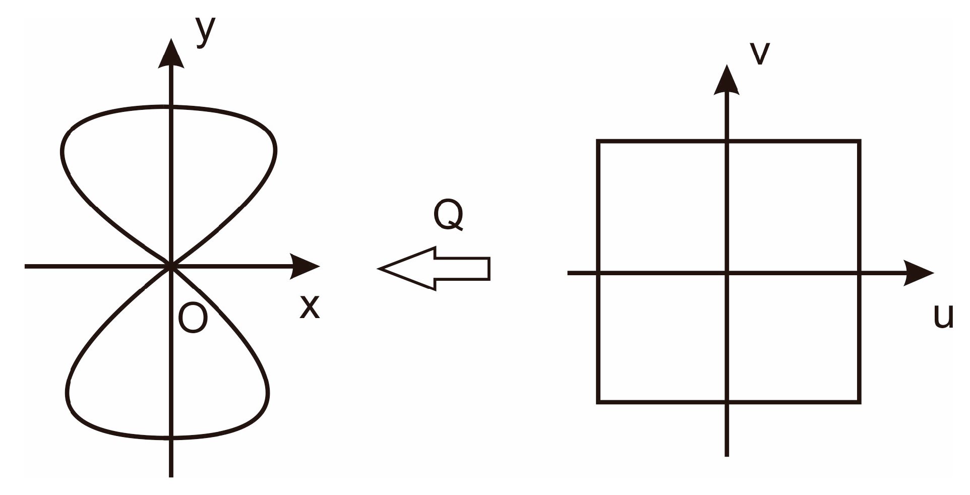
7.2. Monoidal Transform

In order to realize the basic idea for general knots and for K/C elements, we introduce the concept of monoidal transform [61,62,63,64,65,66,67,68,69,70,71,72,73,74,75]. The monoidal categories as well as monoidal transforms are related with braided categories, monoidal equivalence of quantum group, Yang–Baxter equations, and invariants of knots and manifolds [61,62,63,64,65,66,67,68,69,70,71,72,73,74,75,76,77,78,79,80]. We consider a 2-dimensional complex manifold (real 4-dimensional manifold) M.
Take a point P0, we choose a local coordinate U ε ( P 0 ) ( = { ( x , y ) | x 2 + y 2 < ε } ) . A complex manifold U ^ ε ( P 0 ) is made to satisfying the following condition: There exists a mapping (see Figure 14)
Q P 0 : U ^ ε ( P 0 ) U ε ( P 0 )
(i)
Q−1(P0) ≅ Ρ1 (complex projective space)
(ii)
Q P 0 : U ^ ε ( P 0 ) P U ε ( P 0 ) { P 0 }

7.3. Complex Line Bundle of Monoidal Transformation

In consideration of the following complex line bundle over P: F π P, the tuber neighborhood U ^ ε ( P 0 ) satisfies the conditions (i) and (ii). The construction of   π : F P is given as follows:
Let {V0,V} be the standard local coordinate system of Ρ1: P = V 0 V
V 0 = { v | | v | < + } V = { v | | v | < + }
ν ν = 1
By use of the identification
Mathematics 09 00776 i002
{ ν ν = 1 u = ν u
We have a complex line bundle:
F = π 1 ( V 0 ) π 1 ( V )

7.4. Construction of Monoidal Transform

Putting
U ^ ε = U ^ ε ( 0 ) U ^ ε ( ) U ^ ε ( 0 ) = { ( u , ν ) | | u | 2 + | u ν | 2 < ε } U ^ ε ( ) = { ( u , ν ) | | u | 2 + | u ν | 2 < ε }
and { x = u ν y = u on U ^ ε ( 0 ) ; { x = u y = u ν on U ^ ε ( ) ,
We have the desired mapping
Q P 0 : U ^ ε ( P 0 ) U ε ( P 0 )
This is the direct calculation and may be omitted.
By the condition (ii), a monoidal transformation can be introduced,
Q P 0 : M ˜ M
which satisfies the conditions (i) and (ii) above.
Remark 4.
We make stress on the following fact: Even if M = C2 (= R4), the manifold M ˜ is not Euclidean and non-trivial topology appears.

7.5. Basic Notations on Trivialization

For the definition of the concept of trivialization, we begin with some basic notations:
(1)
Trivial elements of exponential type
A direct sum of elements of exponential type of basic 1-form:
exp ( I 3 D ) ~ ~ ~ ~ ~ ~ ~ ~ ~ ~ ~ ~ ~ ~ ~ = i = 1 m [ exp Γ i exp Γ ¯ i ]
is called trivial element. The following mapping:
F : exp ( I 3 D ) ~ ~ ~ ~ ~ ~ ~ ~ ~ ~ ~ ~ ~ ~ ~ [ exp ( Γ 1 ) exp ( Γ m ) ] [ exp ( Γ ¯ m ) exp ( Γ ¯ 1 ) ]
is called generation mapping.
(2)
K/C mapping
The set of K/C elements on a manifold M is denoted by K/C(M). Then, we have
K / C ( M ) = { γ X γ | γ M . X γ C l ( I 3 D )   o n   γ }
where X γ is the direct sum of algebras of exponential type.
X γ = j = 1 l X P j ( j ) ,   γ = P 1 P l
Let M and M′ be two manifolds, and let K/C(M) and K/C(M′) be the K/C elements.

7.6. Basic Idea on Trivialization

Before giving to the statement of Theorem, we demonstrate the basic idea on the trivialization by monoidal transforms in the case of basic type. We consider the following configuration:
As have remarked, we may assume that the Riemann surface is realized in P × C and the knot has singularities of normal crossing (Figure 15):
We consider the solution of the Riemann–Hilbert problem:
| W ˜ = exp ( i K Γ 1 ) exp ( i K Γ ¯ 1 ) ( z α 1 ) β 1 ( z α 1 ) β 1
and next make the monoidal transform (Figure 16) at the intersection point c1 in Figure 15:
( w = u v t = v )
( w = z c 1 ) { w = u t = u v
Then, we have Q w β 1 = { u β 1 ( u v ) β 1 o n o n V 0 V and obtain the following knot (Figure 17):
Therefore, we can make the following identification (Figure 18):
and have the “trivialization”:
exp ( Γ 1 Γ ¯ 1 ) = F Q ( exp Γ 1 exp Γ ¯ 1 )
Then we can prove the following Theorem:
Theorem III.
For an arbitrary K/C element γ X on M, we can construct a trivialization on a four-dimensional manifold M ˜ by monoidal transform trivialization.
Proof of Theorem III is given in Appendix B.
Finally, the trivialization mapping can be constructed in the explicit manner for the transfer matrices V = V1V2V3. The process can be performed in a completely analogous manner, but it is much more complicated, as there are many products of knots.
Remark 5.
Decomposing the trivialization into Clifford algebra and its conjugate algebra, we have Z ˜ γ ˜ and Z ˜ ¯ γ ˜ . Then it is seen that Z ˜ γ ˜ is the desired trivialization: F ( Z ˜ γ ˜ ) = Z γ .
As mentioned in the previous sections, there exist normal knots γ (or links), which are generated by lattice points. Furthermore, the Pauli matrices themselves may be treated as crossings, which contribute the fine structure of the topology. The topological structure of the ferromagnetic 3D Ising model is much more complicated than the examples above. Nevertheless, the trivialization procedure is in an analogous manner, and it can be generalized to be appropriate for any knots (and links) which fit with the partition function (together with normal knots/links γ in lattice points) of the 3D Ising lattice. The monoidal transform utilized here for trivialization of knots consist with the Clifford algebra approach developed in [3,4,8], in which the topology theory [57,58] is employed to take into account of the contribution of non-trivial knots to physical properties of the 3D Ising model, and the generalized Yang–Baxter equations (i.e., the so-called tetrahedron equations) [76,77,78,79,80], corresponding to a Reidemeister move of type III, are used to guarantee the integrability of the system [4]. However, the generalized Yang–Baxter equations [76,77,78,79,80] involve not only the Reidemeister moves, but also the disconnection and fusion of crossings (which can be mapped to the creation and annihilation of spins or particles). Furthermore, the tetrahedron equations are highly overdetermined and constraints must be imposed on the variables of each local weight to allow for a solution [79]. These make the difficulties of explicitly solving the 3D Ising model. In [8], we introduced a local transformation as a topological transformation to deal with the crossings in the 3D Ising model, in order to satisfy the requirements of the tetrahedron equations and to take into account the contribution of these crossings to the physical properties. Meanwhile, we utilized the Largest Eigenvalue Principle that only the largest eigenvalue contributes dominantly to the partition function of the 3D Ising model in the thermodynamic limit. With this constraint, we pick up the desired solution among all 2nl possible solutions in 2nl sub-spaces produced by the direct product of all the sub-transfer matrices. The combination of the local transformation and the Largest Eigenvalue Principle solves the problems of overdetermined tetrahedron equations. The exact solution we found is K K * = K K + K K + K K [3], which is a star–triangle relationship and a solution of the tetrahedron equations and also the Yang–Baxter equations [4,8].

8. Construction of Solution to the Zhang’s Conjecture 1

With the preliminaries in the previous sections, we can construct the trivialization for the Zhang’s conjecture 1 in the following steps:
(1)
We assume that a knot γ is given on the lattice: γ = {Pi}, where Pi is on the lattice points.
(2)
We take a partition function which is defined by the transfer matrices V1, V2, and V3. The members are denoted by V(i) (i = 1,2,…, M).
(3)
We distribute V(i) (i = 1,2,…, M) on knot points Pi of γ, and then have K/C knots Zγ = (γ, X), with X = {V(i)}.
(4)
Making the K/C algebra, we make the conjugate element Z ¯ γ ¯ = ( γ ¯ , X ¯ ) and introduce a K/C knot σ ( Z γ , Z ¯ γ ¯ )
(5)
After realization of the knot σ ( Z γ , Z ¯ γ ¯ ) on a Riemann surface, we can formulate the Riemann–Hilbert problem for the representation.
(6)
We find the solution to the problem with regular singularities at the knot points of the realized knot on the Riemann surface which is denoted by [ Z γ r e g , Z ¯ γ ¯ r e g ] .
(7)
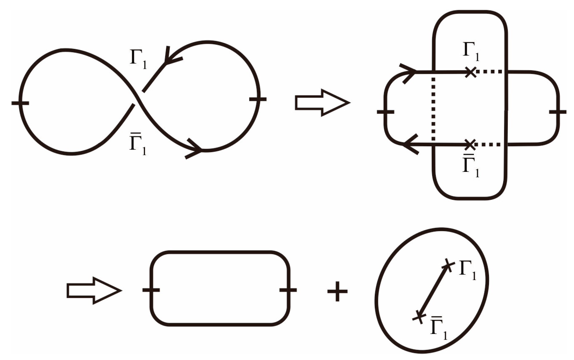
Applying the monoidal transforms at the knot points, we obtain the trivialization [ Z ˜ γ r e g , Z ¯ ˜ γ ¯ r e g ] , to eliminate the singularities from knots.
Summarizing the procedures of this paper, we have proved the following Theorem.
Main Theorem:
The Zhang’s conjecture 1 proposed in [3] can be solved. Namely, for a given K/C knot which is given by the partition function of the ferromagnetic 3D Ising model in the zero external field, we can make the trivialization by use of monoidal transform trivialization.

9. Conclusions

In conclusion, we have developed a method of Riemann–Hilbert problem for Zhang’s conjecture 1 proposed in [3], regarding to the trivialization of topological structure, for the ferromagnetic 3D Ising model in the zero external field. Three claims are formulated in form of Theorems: (I) The partition function Z of the ferromagnetic 3D Ising model in the zero external field can be generated not only by spin alignments, but also by knots. In between these knots one has components which have a complicated topological structure that is contributed by nonlinear terms in the transfer matrices V3. (II) In order to relax this complicated structure, realizations of knots are produced on a four-dimensional Riemann manifold, which are formulated in the Riemann–Hilbert problem for the representation. (III) The monoidal transformations are applied at the knot intersection (singular) points, eliminating these from knots, thus producing the trivialization of the knots. The immediate consequence of these claims is the main theorem that the Zhang’s conjecture 1 proposed in [3] has been proved. The explicit expression for the resulting partition function Z have not been provided directly by the present procedure of the Riemann–Hilbert problem and the monoidal transformations. The partition function Z in a 4-fold integral form was presented in Equation (49) in [3] (see also Equation (24) in [4]) based on the Zhang’s two conjectures, which was proven to be correct in [8] by a Clifford algebra approach. The thermodynamical properties (including the free energy, the specific heat, the spontaneous magnetization, the spin correlation, the susceptibility, as well as the critical exponents) of the ferromagnetic 3D Ising model in the zero external field are derived explicitly in [3]. However, attention should be paid on using the present procedure to demonstrate rigorous formulation for the non-trivial knots’ components of the partition function Z. A subsequent paper, on the method of Riemann–Hilbert problem for Zhang’s conjecture 2, regarding to the generation of topological phases, will be published soon [81]. Furthermore, because the exact solution for the antiferromagnetic 3D Ising model with all the negative interactions but without frustration in the zero external field has the same formula as the exact solution obtained in [3,4,8], the results in [3,4,8] for the ferromagnetic 3D Ising model in the zero external field are suitable for the antiferromagnetic 3D Ising model without frustration.
It should be emphasized that the procedures developed in [8] and this work, to deal with the non-trivial topological structures in the ferromagnetic 3D Ising lattices in the zero external field, and the exact solution obtained in [3], are valid for any positive inverse temperature β = 1/(kBT) > 0 (including the area of phase transitions, βc), where the non-trivial topological structures exist. It is clear now that the non-trivial topological structures (knots) contribute additional terms to the partition function and the physical properties (such as the free energy, the specific heat, the spontaneous magnetization, the spin correlation, the susceptibility, the critical exponents). Any approaches based on only local environments, such as conventional low-temperature expansions, conventional high-temperature expansions, Monte Carlo simulations, Renormalization Group, etc., are not exact, because these approximative approaches miss the contributions of knots. The conventional high-temperature expansions work only at/near infinite temperature β = 0, where only the trivial topological structure exists. Our procedures in [3,4,8] and the present work indicate that it is necessary to introduce an additional dimension (the time) to trivialize the knots and take into account their contributions, to achieve the exact solution of the 3D Ising models. The temperature–time duality in the 3D Ising model can be seen by inspecting the resemblance between the density operator in quantum statistical mechanics and the evolution operator in quantum field theory, with the mapping β = (kBT)−1 → it = τ [82,83,84]. In [84], Zhang and March pointed out that besides the Wick rotation, which represents the temperature as the imaginary time, we have to introduce also the time for the time average and for untying the knots (see also in [3,4,8] and this work). Therefore, one has to deal with the topological quantum field theory within a (3 + 2) or (4 + 1)-dimensional framework [85]. With Wick representation, the ε-expansions [86,87,88] start from four dimensions and do not account the non-trivial topological contributions, which are still in the approximative level. It can be improved by accounting the contributions of the non-trivial topological structure in the (3 + 2) or (4 + 1)-dimensional framework. Finally, we would like to notice that our work illustrates that the 3D Ising spin system can serve as a platform for describing a sensible interplay in between the physical properties of interacting many-body systems, algebra, topology, and geometry.

Author Contributions

Propose the project, Z.Z.; Physical ideas, Z.Z.; Mathematical methods, O.S; Proofs of Theorems, O.S. and Z.Z.; Writing the paper, O.S. and Z.Z. All authors have read and agreed to the published version of the manuscript.

Funding

This research was funded by the National Natural Science Foundation of China grant number 52031014. The APC was funded by the National Natural Science Foundation of China.

Institutional Review Board Statement

Not applicable.

Informed Consent Statement

Not applicable.

Data Availability Statement

The data is available on reasonable request from the corresponding author.

Conflicts of Interest

The authors declare no conflict of interest.

Appendix A. Proof of Theorem II

Appendix A.1. Construction of the Representation (Proof of (1) in Theorem II)

We give the construction ρ ˜ which is given in (1) of Theorem II and make the twisted knot from the standard knot. Then the Riemann–Hilbert problem can be formulated. We put
Γ i = C C s ( i ) 1 1
Γ ¯ i = C ¯ C ¯ s ¯ ( i ) 1 ¯ 1 ¯
(i = 1, 2, …, m)
(1)
The case of basic type
We make the knot of twisted type from the knot of standard type (Figure A1):
Figure A1. Making the knot of twisted type from the knot of standard type.
Mathematics 09 00776 g0a1
Next construct a Riemann surface. We prepare two branch points α 1 , α 1 in the following configuration and construct the knot. As the knot is a 1 + a 1 , it becomes in the configuration (Figure A2).
Figure A2. Construct the knot on a Riemann surface.
Mathematics 09 00776 g0a2
The over (under) going path from P (respective Q) through P1 to Q (respective P) is denoted by γ 1 ( + ) (respective γ 1 ( ) ). We put γ 1 = γ 1 ( + ) γ 1 ( ) .
(2)
The case of simple/multi-type
We choose the knot of multi-type with the following orientation of twist type: We consider the case m = 4 (see Figure A3).
Figure A3. The knot of multi-type with the following orientation of twist type for the case m = 4.
Mathematics 09 00776 g0a3
The over (under) going path from P (respective Q) to Q (respective P) is denoted by γ m ( + ) , γ m ( ) ) and γ m = γ m ( + ) γ m ( ) . We choose a realization on a Riemann surface in the following manner:
(i)
Choose a Riemann surface (Figure A4)
Figure A4. A realization on a Riemann surface.
Mathematics 09 00776 g0a4
(ii)
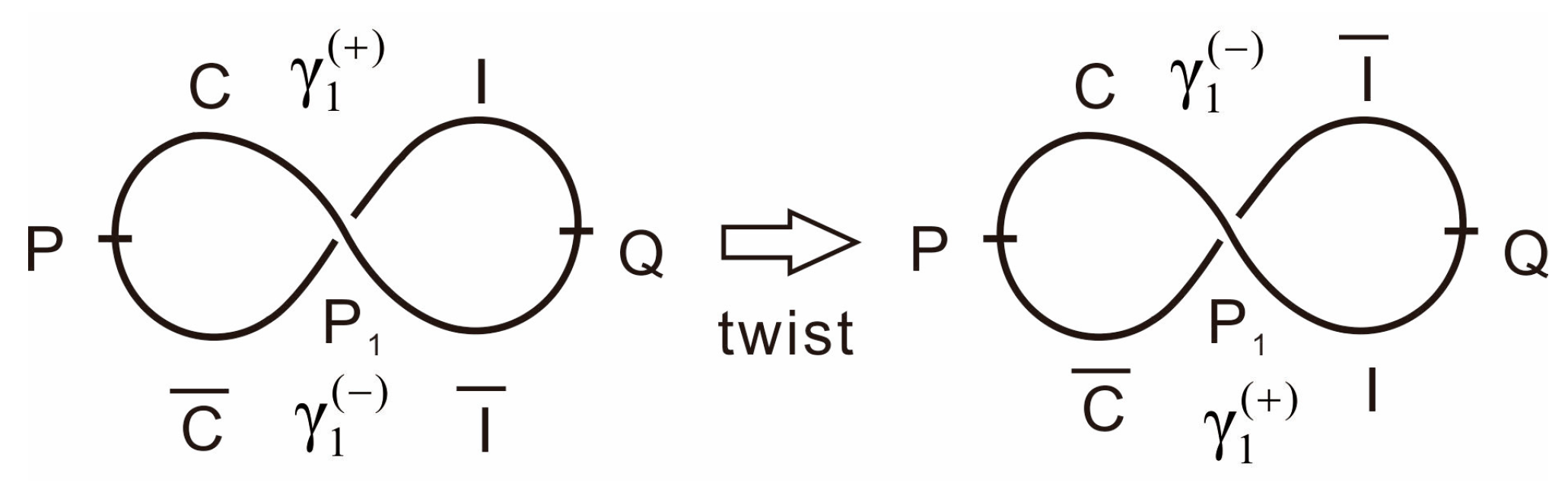
Make a realization of γ by use of association of twisted type (Figure A5).
Figure A5. Make a realization of a knot γ by use of association of twisted type.
Mathematics 09 00776 g0a5
The approach above can be applied for the general case of m.

Appendix A.2. Construction of the Solutions (Proof of (2) in Theorem II)

The solution of Riemann–Hilbert problem can be constructed. We give the solutions in the cases of basic types I and II, separately. We have to pay attention to the method of the construction. We construct the solutions both for positive elements and negative elements at the same time. Therefore, the solutions are considered in the universal K/C algebra.
(1)
The solution for the basic form of type I
The solution is given as follows:
Putting
F = ( z α 1 ) β 1 ( z α 1 ) β 1 ( β 1 , β 1 = ± 1 / 2 ) ,
we have
{ γ 1 * F = γ 1 ( ) * γ 1 ( + ) * F γ 1 ( + ) * = e 2 π i β 1 exp ( i K Γ 1 ) γ 1 ( ) * = e 2 π i β 1 exp ( i K Γ ¯ 1 )
(2)
The solution for the basic form of type II
Following the method of the Röhrl’s solution for the Riemann–Hilbert problem [59], we have the solution
F ( z ) = i = 1 m ( z α i ) β i ( z α 1 ) β 1 ( β i , β 1 = ± 1 / 2 )
Then, we have the following representation: ρ ˜ ( γ m ( + ) γ m ( ) ) = ρ ˜ ( γ m ( + ) ) ρ ˜ ( γ m ( ) ) , where
{ ρ ˜ ( γ m ( + ) ) = i = 1 m e 2 π i β i exp ( i m K Γ 1 Γ 2 Γ m ) ρ ˜ ( γ m ( ) ) = i = 1 m e 2 π i β i exp ( i m K Γ ¯ m Γ ¯ m 1 Γ ¯ 1 )
(3)
The general type
In this case, there are two kinds of intersection points: (1) {a1, …an} are the singularities arising from the knot of multi-type; (2) {b1, …, bm} are the singularities arising from the part of the given non-trivial knot. For the simplest sake, we write the sequence {an, bm} as {ck}, k = 1, 2, …, n+m, and put Γ i = Γ ¯ i = 1 for bi, we can rewrite them {ck}. { Γ k , Γ ¯ k } . Then, following the procedure above, we can formulate the Riemann–Hilbert problem and find the desired solution. The discussion is completely identical, and it may be omitted.

Appendix B. Proof of Theorem III

We begin with recalling the classification of the knots in the transfer matrices V1, V2, and V3. From the results in Section 4, there are knots of the following types: basic types I and II, product type (and adjoint type). In the following, we construct the trivializations for these basic types and combining the results, the desired trivialization is obtained for the product type.
The configuration of type I can be trivialized by the scheme in the basic idea. We have the following trivialization (Figure A6):
Figure A6. The trivialization of the configuration of type I.
Mathematics 09 00776 g0a6
We construct the trivialization in the case of the configuration type II and m = 3 as the following process (Figure A7).
Figure A7. The trivialization of the configuration of type II and m = 3.
Mathematics 09 00776 g0a7
The desired trivialization is given by
( exp Γ 1 exp Γ ¯ 1 ) ( exp Γ 2 exp Γ ¯ 2 ) ( exp Γ 3 exp Γ ¯ 3 )
We treat the product type by the choice of an example:
exp ( i K * Γ 2 k 1 Γ 2 k ) exp ( i K Γ 2 l Γ 2 l + 1 ) exp ( i n K Γ 2 j ( Γ 2 j + 1 Γ 2 j + 2 Γ 2 j + 2 m 2 ) Γ 2 j + 2 m 1 )
Following the results of Theorem I, one can obtain the following configuration (Figure A8):
Figure A8. Schematic illustration of a configuration of braids as an example.
Mathematics 09 00776 g0a8
The trivialization can be made for each block (I), (II), or (III), separately, and joint each construction. The joint is given as follows: At each point Pi, we have no information on knot structures. At each point, we associate the trivial matrix which is denoted by Γ ( P i ) and Γ ¯ ( P i ) , make extensions, for example, the extension is given at Pi in the following manner and other cases are treated in a completely analogous manner (Figure A9).
Figure A9. The trivialization of a configuration.
Mathematics 09 00776 g0a9
Then, we see that
exp [ ( Γ ( P 1 ) Γ 2 j 1 Γ 2 j ) ( Γ ¯ 2 j Γ ¯ 2 j 1 Γ ¯ ( P 1 ) ) ] = exp [ ( Γ 2 j 1 Γ 2 j ) ( Γ ¯ 2 j Γ ¯ 2 j 1 ) ]
Therefore, the representation does not change, i.e., is invariant. The monoidal transform becomes as follows (see Figure A10):
Figure A10. The monoidal transform for a configuration.
Mathematics 09 00776 g0a10
Here, the dotted circle implies the S2 (≅P1) which does not contribute to the partition functions. Thus, we may omit it.
Performing the process to P2, P3, the following diagram is obtained by monoidal transforms (Figure A11):
Figure A11. The monoidal transform for a configuration.
Mathematics 09 00776 g0a11

References

  1. Ising, E. Report on the theory of ferromagnetism. Z. Phys. 1925, 31, 253–258. [Google Scholar] [CrossRef]
  2. Onsager, L. Crystal Statistics I: A two-dimensional model with an order-disorder transition. Phys. Rev. 1944, 65, 117–149. [Google Scholar] [CrossRef]
  3. Zhang, Z.D. Conjectures on the exact solution of three-dimensional (3D) simple orthorhombic Ising lattices. Phil. Mag. 2007, 87, 5309–5419. [Google Scholar] [CrossRef] [Green Version]
  4. Zhang, Z.D. Mathematical structure of three-dimensional (3D) Ising model. Chin. Phys. B 2013, 22, 030513. [Google Scholar] [CrossRef] [Green Version]
  5. Newell, G.F.; Montroll, E.W. On the theory of the Ising model with ferromagnetism. Rev. Mod. Phys. 1953, 25, 353–389. [Google Scholar] [CrossRef]
  6. Ławrynowicz, J.; Marchiafava, S.; Niemczynowicz, A. An approach to models of order-disorder and Ising lattices. Adv. Appl. Clifford Algebra 2010, 20, 733–743. [Google Scholar] [CrossRef]
  7. Ławrynowicz, J.; Suzuki, O.; Niemczynowicz, A. On the ternary approach to Clifford structures and Ising lattices. Adv. Appl. Clifford Algebra 2012, 22, 757–769. [Google Scholar] [CrossRef] [Green Version]
  8. Zhang, Z.D.; Suzuki, O.; March, N.H. Clifford algebra approach of 3D Ising model. Adv. Appl. Clifford Algebra 2019, 29, 12. [Google Scholar] [CrossRef] [Green Version]
  9. Zhang, Z.D. Computational complexity of spin-glass three-dimensional (3D) Ising model. J. Mater. Sci. Tech. 2020, 44, 116–120. [Google Scholar] [CrossRef]
  10. Zhang, Z.D. Exact solution of two-dimensional (2D) Ising model with a transverse field: A low-dimensional quantum spin system. Phys. E 2021, 128, 114632. [Google Scholar] [CrossRef]
  11. Wu, F.Y.; McCoy, B.M.; Fisher, M.E.; Chayes, L. Comment on a recent conjectured solution of the three-dimensional Ising model. Phil. Mag. 2008, 88, 3093–3095. [Google Scholar] [CrossRef]
  12. Wu, F.Y.; McCoy, B.M.; Fisher, M.E.; Chayes, L. Rejoinder to the Response to “Comment on a recent conjectured solution of the three-dimensional Ising model”. Phil. Mag. 2008, 88, 3103. [Google Scholar] [CrossRef]
  13. Perk, J.H.H. Comment on “Conjectures on exact solution of three-dimensional (3D) simple orthorhombic Ising lattices”. Phil. Mag. 2009, 89, 761–764. [Google Scholar] [CrossRef] [Green Version]
  14. Perk, J.H.H. Rejoinder to the Response to the Comment on “Conjectures on exact solution of three-dimensional (3D) simple orthorhombic Ising lattices”. Phil. Mag. 2009, 89, 769–770. [Google Scholar] [CrossRef] [Green Version]
  15. Perk, J.H.H. Comment on “Mathematical structure of the three—dimensional (3D) Ising model”. Chinese Phys. B 2013, 22, 131507. [Google Scholar] [CrossRef] [Green Version]
  16. Fisher, M.E.; Perk, J.H.H. Comments concerning the Ising model and two letters by N.H. March. Phys. Lett. A 2016, 380, 1339–1340. [Google Scholar] [CrossRef] [Green Version]
  17. El-Showk, S.; Paulos, M.F.; Poland, D.; Rychkov, S.; Simmons-Duffin, D.; Vichi, A. Solving the 3d Ising model with the conformal bootstrap II. -Minimization and precise critical exponents. J. Stat. Phys. 2014, 157, 869–914. [Google Scholar] [CrossRef] [Green Version]
  18. Zhang, Z.D. Response to “Comment on a recent conjectured solution of the three-dimensional Ising model”. Phil. Mag. 2008, 88, 3097–3101. [Google Scholar] [CrossRef] [Green Version]
  19. Zhang, Z.D. Response to the Comment on “Conjectures on exact solution of three dimensional (3D) simple orthorhombic Ising lattices”. Phil. Mag. 2009, 89, 765–768. [Google Scholar] [CrossRef] [Green Version]
  20. Lou, S.L.; Wu, S.H. Three-dimensional Ising model and transfer matrices. Chin. J. Phys. 2000, 38, 841–854. [Google Scholar]
  21. Istrail, S. Universality of intractability for the partition function of the Ising model across non-planar lattices. In Proceedings of the 32nd ACM Symposium on the Theory of Computing, Portland, OR, USA, 21–23 May 2000; pp. 87–96. [Google Scholar]
  22. Gallavotti, G.; Miracle-Solé, S. Correlation functions of a lattice system. Commun. Math. Phys. 1968, 7, 274–288. [Google Scholar] [CrossRef]
  23. Lebowitz, J.L.; Penrose, O. Analytic and clustering properties of thermodynamic functions and distribution functions for classical lattice and continuum systems. Commun. Math. Phys. 1968, 11, 99–124. [Google Scholar] [CrossRef]
  24. Ruelle, D. Statistical Mechanics. In Rigorous Results; Benjamin: New York, NY, USA, 1969. [Google Scholar]
  25. Griffiths, R.B. Phase Transitions and Critical Phenomena; Domb, C., Green, M.S., Eds.; Academic Press: London, UK, 1972; Volume 1, Chapter 2, sections III and IV D. [Google Scholar]
  26. Miracle-Solé, S. Theorems on phase transitions with a treatment for the Ising model. In Lecture Notes in Physics; Springer: New York, NY, USA, 1976; Volume 54, p. 189. [Google Scholar]
  27. Sinai, Y.G. Theory of Phase Transitions: Rigorous Results; Pergamon Press: Oxford, UK, 1982; Chapter II. [Google Scholar]
  28. Yang, C.N.; Lee, T.D. Statistical theory of equations of state and phase transitions.1. Theory of condensation. Phys. Rev. 1952, 87, 404–409. [Google Scholar] [CrossRef]
  29. Lee, T.D.; Yang, C.N. Statistical theory of equations of state and phase transitions. 2. Lattice gas and Ising model. Phys. Rev. 1952, 87, 410–419. [Google Scholar] [CrossRef]
  30. Kaupuzs, J.; Melnik, R.V.N.; Rimsans, J. Corrections to finite–size scaling in the 3D Ising model based on non–perturbative approaches and Monte Carlo simulations. Inter. J. Modern Phys. C 2017, 28, 1750044. [Google Scholar] [CrossRef] [Green Version]
  31. Zhang, Z.D.; March, N.H. Three-dimensional (3D) Ising universality in magnets and critical indices at fluid-fluid phase transition. Phase Transit. 2011, 84, 299–307. [Google Scholar] [CrossRef]
  32. Klein, D.J.; March, N.H. Critical exponents in D dimensions for the Ising model, subsuming Zhang’s proposals for D = 3. Phys. Lett. A 2008, 372, 5052–5053. [Google Scholar] [CrossRef]
  33. March, N.H. Crucial combinations of critical exponents for liquids-vapour and ferromagnetic second-order phase transitions. Phys. Chem. Liquids 2014, 52, 697–699. [Google Scholar] [CrossRef]
  34. March, N.H. Similarities and contrasts between critical point behavior of heavy fluid alkalis and d-dimensional Ising model. Phys. Lett. A 2014, 378, 254–256. [Google Scholar] [CrossRef]
  35. March, N.H. Toward a final theory of critical exponents in terms of dimensionality d plus universality class n. Phys. Lett. A 2015, 379, 820–822. [Google Scholar] [CrossRef]
  36. March, N.H. Unified theory of critical exponents generated by the Ising Hamiltonian for discrete dimensionalities 2, 3 and 4 in terms of the critical exponent η. Phys. Chem. Liquids 2016, 54, 127–129. [Google Scholar] [CrossRef]
  37. Ławrynowicz, J.; Nowak-Kepczyk, M.; Suzuki, O. Fractals and chaos related to Ising-Onsager-Zhang lattices versus the Jordan-von Neumann-Wigner procedures. Quaternary approach. Inter. J. Bifurcation Chaos 2012, 22, 1230003. [Google Scholar] [CrossRef]
  38. Ławrynowicz, J.; Suzuki, O.; Niemczynowicz, A.; Nowak-Kepczyk, M. Fractals and chaos related to Ising-Onsager-Zhang lattices. Quaternary Approach vs. Ternary Approach. Adv Appl Clifford Alg 2020, 29, 45. [Google Scholar] [CrossRef] [Green Version]
  39. Kaupuzs, J. Power law singularities in n-vectur models. Canadian J. Phys. 2012, 90, 373–382. [Google Scholar] [CrossRef]
  40. Kaupuzs, J.; Melnik, R.V.N.; Rimsans, J. Scaling regimes and singularity of specific heat in the 3D Ising model. Commun. Comput. Phys. 2013, 14, 355–369. [Google Scholar] [CrossRef]
  41. Grigalaitis, R.; Lapinskas, S.; Banys, J.; Tornau, E.E. On ergodic relaxation time in the three-dimensional Ising model. Lith. J. Phys. 2013, 53, 157–162. [Google Scholar] [CrossRef]
  42. Warda, K.; Wojtczak, L. The magnetic question of state and transport properties in reduced dimensions. Acta Phys. Pol. A 2017, 131, 878–880. [Google Scholar] [CrossRef]
  43. Zeyad, A.Z. Some new linear representations of matrix quaternions with some applications. J. King Saud Univ. Sci. 2019, 31, 42–47. [Google Scholar]
  44. Zeng, D.F. Emergent time axis from statistic/gravity dualities. arXiv 2014, arXiv:1407.8504. [Google Scholar]
  45. Cheng, J.; Di, Z.R. Collective behavior and spin model on complex networks. Adv. Mech. 2008, 38, 733–750. [Google Scholar]
  46. Zhang, O.B.; Fan, Y.; Di, Z.R. Influence of balanced structure on the spread of public opinion in signed networks. Complex Syst. Complex. Sci. 2019, 16, 1672–3813. [Google Scholar]
  47. Lu, Z.M.; Si, N.; Wang, Y.N.; Zhang, F.; Meng, J.; Miao, H.L.; Jiang, W. Unique magnetism in different sizes of center decorated tetragonal nanoparticles with the anisotropy. Phys. A 2019, 523, 438–456. [Google Scholar] [CrossRef]
  48. Wang, X.S.; Zhang, F.; Si, N.; Meng, J.; Zhang, Y.L.; Jiang, W. Unique magnetic and thermodynamic properties of a zigzag graphene nanoribbon. Phys. A 2019, 527, 121356. [Google Scholar] [CrossRef]
  49. Yang, M.; Wang, W.; Li, B.C.; Wu, H.J.; Yang, S.Q.; Yang, J. Magnetic properties of an Ising ladder-like graphene nanoribbon by using Monte Carlo method. Phys. A 2020, 539, 122932. [Google Scholar] [CrossRef]
  50. Li, Q.; Li, R.D.; Wang, W.; Geng, R.Z.; Huang, H.; Zheng, S.J. Magnetic and thermodynamic characteristics of a rectangle Ising nanoribbon. Phys. A 2020, 555, 124741. [Google Scholar] [CrossRef]
  51. Ghorai, S.; Skini, R.; Hedlund, D.; Ström, P.; Svedlindh, P. Field induced crossover in critical behaviour and direct measurement of the magnetocaloric properties of La0.4Pr0.3Ca0.1Sr0.2MnO3. Sci. Rep. 2020, 10, 19485. [Google Scholar] [CrossRef]
  52. Paszkiewicz, A.; Węrzyn, J. Responsiveness of the sensor network to alarm events based on the Potts model. Sensors 2020, 20, 6979. [Google Scholar] [CrossRef]
  53. Ma, S.Y.; Zhang, H.Z. Opinion expression dynamics in social media chat groups: An integrated quasi-experimental and agent-based model approach. Complexity 2021, 2304754. [Google Scholar] [CrossRef]
  54. Zhang, Z.D. The nature of three dimensions: Non-local behavior in the three-dimensional (3D) Ising model. J. Phys. Conf. Ser. 2017, 827, 012001. [Google Scholar] [CrossRef] [Green Version]
  55. Zhang, Z.D. Topological effects and critical phenomena in the three-dimensional (3D) Ising model, Chapter 27. In Many-Body Approaches at Different Scales: A Tribute to Norman H. March on the Occasion of his 90th Birthday; Angilella, G.G.N., Amovilli, C., Eds.; Springer: New York, NY, USA, 2018. [Google Scholar]
  56. Kaufman, B. Crystal Statistics II: Partition function evaluated by spinor analysis. Phys. Rev. 1949, 76, 1232–1243. [Google Scholar] [CrossRef]
  57. Kauffman, L.H. Knots and Physics, 3rd ed.; World Scientific Publishing Co. Pte. Ltd.: Singapore, 2001. [Google Scholar]
  58. Kauffman, L.H. Knot Theory and Physics. In The Encyclopedia of Mathematical Physics; Francoise, J.P., Naber, G.L., Tsun, T.S., Eds.; Elsevier: Amsterdam, The Netherlands, 2007. [Google Scholar]
  59. Röhrl, H. Das Riemannsch—Hilbertsche Problem der Theorie der Linieren Differentialgleichungen. Math. Ann. 1957, 133, 1–25. [Google Scholar]
  60. Suzuki, O. The Problem of Riemann and Hilbert and the Relations of Fuchs in Several Complex Variables, Lecture Notes in Math; Springer: Berlin, Germany, 1977; Volume 712, pp. 325–364. [Google Scholar]
  61. Lipman, J. Desingularization of two-dimensional schemes. Ann. Math. 1978, 107, 151–207. [Google Scholar] [CrossRef]
  62. Hartshone, R. Algebraic Geometry, Graduate Texts in Math; Springer: New York, NY, USA, 1977; p. 52. [Google Scholar]
  63. Kock, A. Strong functors and monoidal monads. Arch. Math. 1972, 23, 113–120. [Google Scholar] [CrossRef]
  64. Baez, J.C. Higher dimensional algebra I. braided monoidal 2-categories. Adv. Math. 1996, 121, 196–244. [Google Scholar] [CrossRef] [Green Version]
  65. Bespalov, Y.N. Crossed modules and quantum groups in braided categories. Appl. Categ. Struct. 1997, 5, 155–204. [Google Scholar] [CrossRef]
  66. Bespalov, Y.; Drabant, B. Hopf (bi-)modules and crossed modules in braided monoidal categories. J. Pure Appl. Algebra 1998, 123, 105–129. [Google Scholar] [CrossRef] [Green Version]
  67. Majid, S. Braided groups. J. Pure Appl. Algebra 1993, 86, 187–221. [Google Scholar] [CrossRef] [Green Version]
  68. Kapranov, M.; Voevodsky, V. Braided monoidal 2-categories and Manin-Schechtman higher braid groups. J. Pure Appl. Algebra 1994, 92, 241–267. [Google Scholar] [CrossRef] [Green Version]
  69. Balteanu, C.; Fiedorowicz, Z.; Schwänzl, R.; Vogt, R. Iterated monoidal categories. Adv. Math. 2003, 176, 277–349. [Google Scholar] [CrossRef] [Green Version]
  70. Joyal, A.; Street, R.; Verity, D. Traced monoidal categories. Math. Proc. Gamb. Phil. Soc. 1996, 119, 447–468. [Google Scholar] [CrossRef]
  71. Bichon, J.; Rijdt, A.D.; Vaes, S. Ergodic coactions with large multiplicity and monoidal equivalence of quantum groups. Commun. Math. Phys. 2006, 262, 703–728. [Google Scholar] [CrossRef] [Green Version]
  72. Etingof, P.; Varchenko, A. Solutions of the quantum dynamical Yang–Baxter equation and dynamical quantum groups. Commun. Math. Phys. 1998, 196, 591–640. [Google Scholar] [CrossRef] [Green Version]
  73. Yetter, D.N. Quantum groups and representations of monoidal categories. Math. Proc. Camb. Phil. Soc. 1990, 108, 261–290. [Google Scholar] [CrossRef]
  74. Majid, S. Transmutation theory and rank for quantum braided groups. Math. Proc. Camb. Phil. Soc. 1993, 113, 45–70. [Google Scholar] [CrossRef]
  75. Nikshych, D.; Turaev, V.; Vainerman, L. Invariants of knots and 3-manifolds from quantum groupoids. Topol. Appl. 2003, 127, 91–123. [Google Scholar] [CrossRef] [Green Version]
  76. Yang, C.N. Some exact results for the many-body problem in one dimension with repulsive delta-function interaction. Phys. Rev. Lett. 1967, 19, 1312–1315. [Google Scholar] [CrossRef]
  77. Baxter, R.J. Partition function of the eight-vertex lattice model. Ann. Phys. 1972, 70, 193–228. [Google Scholar] [CrossRef]
  78. Zamolodchikov, A.B. Tetrahedron equations and the relativistic S-matrix of straight-strings in 2+1 dimensions. Commun. Math. Phys. 1981, 79, 489–505. [Google Scholar] [CrossRef]
  79. Jaekel, M.T.; Maillard, J.M. Symmetry-relaxations in exactly soluble models. J. Phys. A 1982, 15, 1309–1325. [Google Scholar] [CrossRef]
  80. Stroganov, Y.G. Tetrahedron equation and spin integrable models on a cubic lattice. Theor. Math. Phys. 1997, 110, 141–167. [Google Scholar] [CrossRef]
  81. Zhang, Z.D.; Suzuki, O. A method of Riemann-Hilbert problem for Zhang’s conjecture 2 in a ferromagnetic 3D Ising model: Topological phase. 2021. to be published. [Google Scholar]
  82. Binney, J.J.; Dowrick, N.J.; Fisher, A.J.; Newman, M.E.J. The Theory of Critical Phenomena, An Introduction to the Renormalization Group; Clarendon Press: Oxford, UK, 1992. [Google Scholar]
  83. Francesco, P.D.; Mathieu, P.; Sénéchal, D. Conformal Field Theory; Springer: New York, NY, USA, 1996. [Google Scholar]
  84. Zhang, Z.D.; March, N.H. Temperature-time duality exemplified by Ising magnets and quantum-chemical many electron theory. J. Math. Chem. 2011, 49, 1283–1290. [Google Scholar] [CrossRef]
  85. Zhang, Z.D. On topological quantum statistical mechanics and topological quantum field theories. to be published.
  86. Wilson, K.G.; Fisher, M.E. Critical exponents in 3.99 dimensions. Phys. Rev. Lett. 1972, 28, 240–243. [Google Scholar] [CrossRef]
  87. Wilson, K.G. Feynman-graph expansion for critical exponents. Phys. Rev. Lett. 1972, 28, 548–551. [Google Scholar] [CrossRef]
  88. Wilson, K.G. The renormalization group and critical phenomena. Rev. Mod. Phys. 1983, 55, 583–600. [Google Scholar] [CrossRef]
Figure 1. A knot γ constructed in the 3D lattice Z3.
Mathematics 09 00776 g001
Figure 2. A knot called basic form of type I, with the element i Γ i Γ ¯ j or i Γ ¯ i Γ j .
Mathematics 09 00776 g002
Figure 3. A knot called basic form of type II, which can be represented as a braid with many crosses (k = 2n).
Mathematics 09 00776 g003
Figure 4. Schemes illustrate three of the braids in the transfer matrix V3 connecting to the lattice points of the knot γ, while the circles of V1 and V2 are not shown for simplicity.
Mathematics 09 00776 g004
Figure 5. A 2-covering Riemann surface Mg made by use of cut-segments where n is even (n = 2m).
Mathematics 09 00776 g005
Figure 6. A 2-covering Riemann surface Mg made by use of cut-segments where n is odd (n = 2m + 1).
Mathematics 09 00776 g006
Figure 7. Construction of the Riemann surface z with the cut along (0∞).
Mathematics 09 00776 g007
Figure 8. The base Riemann surface Mg in P × C as a covering space over P1 in which the knot has a singularity of normal crossing.
Mathematics 09 00776 g008
Figure 9. The realization of knots on the Riemann surface.
Mathematics 09 00776 g009
Figure 10. The realization of knots on the Riemann surface. The dots represent the circle on the lower surface
Mathematics 09 00776 g010
Figure 11. A knot with crossings.
Mathematics 09 00776 g011
Figure 12. The realization of the knot in Figure 11 on the Riemann surface.
Mathematics 09 00776 g012
Figure 13. A mapping for trivialization.
Mathematics 09 00776 g013
Figure 14. A mapping for monoidal transform.
Mathematics 09 00776 g014
Figure 15. A knot with singularities of normal crossing.
Mathematics 09 00776 g015
Figure 16. The monoidal transform at the intersection point c1 in Figure 15.
Mathematics 09 00776 g016
Figure 17. The monoidal transform for trivialization of a knot.
Mathematics 09 00776 g017
Figure 18. Identification of the monoidal transform.
Mathematics 09 00776 g018
Table 1. The knot/Clifford algebra with the product table.
b1 1 ¯ C C ¯
a
111CC
1 ¯ 1 ¯ 1 ¯ C ¯ C ¯
CCC11
C ¯ C ¯ C ¯ 1 ¯ 1 ¯
Publisher’s Note: MDPI stays neutral with regard to jurisdictional claims in published maps and institutional affiliations.

