Modelling of Fuel- and Energy-Switching Prices by Mean-Reverting Processes and Their Applications to Alberta Energy Markets

Abstract

This paper introduces a fuel-switching price to the Alberta market, which is designed for encouraging power plant companies to switch from coal to natural gas when they produce electricity; this has been successfully applied to the European market. Moreover, we consider an energy-switching price which considers power switch from natural gas to wind. We modeled these two prices using five mean reverting processes including a Regime-switching processes, Lévy-driven Ornstein–Uhlenbeck process and Inhomogeneous Geometric Brownian Motion, and estimate them based on multiple procedures such as Maximum likelihood estimation and Expectation-Maximization algorithm. Finally, this paper proves previous results applied to the Albertan Market where the jump modeling technique is needed when modeling fuel-switching data. In addition, it not only gives promising conclusions on the necessity of introducing Regime-switching models to the fuel-switching data, but also shows that the Regime-switching model is better fitted to the data.

1. Introduction

1.1. Overview

The federal government of Canada published “The pan-Canadian approach to pricing Carbon Pollution” in October 2016 aiming at reducing green house gas (GHG) emissions by taxing fossil fuels. There are two carbon tax systems mentioned in it: an explicit price-based system and a cap-and-trade system. The cap-and-trade system gives each company limit tradable allowance for GHG emission, while the explicit price-based system sets a tax price for a fixed carbon emission. In Alberta, we are using the explicit price-based system and the current Carbon levy is $\$50$ per tonne. However, Tombe (2017) [1] found that household electricity bills were expected to rise by $\$150$ when the Carbon levy increased in 2018. Moreover, this tax is going to affect poor households which could increase inequalities in turn (Ambasta and Buonocore, 2018 [2]). This all indicates that this price is imperfect and a correct pricing method is needed for Albertan residents.

Electricity prices are effected by factors such as weather conditions, economic growth, political principles and fuel-switching (Sjim et al., 2006 [3]; Seifert et al., 2008 [4]; Carmona et al., 2009 [5]), where the fuel-switching is the only one that is controllable by the company itself. The term fuel-switching means specifically that for any power plant that is coal fired or gas fired, the company can switch based on price and produce the same quantities of electricity. Since coal price is cheaper than natural gas price but nearly twice as polluting as gas (Arora and Taylor 2014 [6]), we are able to consider potentials of GHG emissions reduction through fuel-switching (Erik Delarue, William D’haeseleer 2006 [7]). This paper introduces a fuel-switching price, which explains how to switch from coal to natural gas when producing electricity, and how this can apply to the Albertan energy market. In the Albertan market, there are examples of power plant companies which are working on fuel switching, such as Transalta’s Coal-to-Gas Conversions Project and Capital Power’s Repowering Genesee Project. We also introduce an energy-switching price which considers a power switch from natural gas to wind. Moreover, note that this paper focuses on different jump and regime-switching mean-reverting stochastic models, where the financial and economic meanings and their applications will be discussed in another paper. We model these two prices using five mean-reverting processes and including regime-switching processes, such as the Lévy-driven Ornstein–Uhlenbeck process and inhomogeneous geometric motion. The estimation of these processes is based on multiple procedures such as maximum likelihood estimation and the expectation-maximization algorithm. This paper also justifies previous results applied to the Albertan energy market showing that the jump modelling technique is needed when modelling fuel-switching data. Finally, the novelty of the paper lies not only in giving a promising conclusion on the necessity of introducing regime-switching models to the fuel-switching data, but also in showing that regime-switching models are better fitted to the data.

This paper is based on several projects and ideas, first introduced in Arrigoni et al., 2019 [8], and then extended in Lu 2020 [9] to consider more stochastic models for fuel-switching and energy-switching prices. We consider inhomogeneous geometric Brownian motion and generate its parameter estimation procedure by using change of time method from Swishchuk 2008 [10]. We also consider the regime-switching models and the original Lévy-driven models. Unlike previous models with a constant volatility, the regime-switching model assumes that the volatility is changing according to each regime and they can switch the value between regimes. The regime-switching models generally consider a business cycle behind our data, with different regimes modelled by a Markov chain that represents different stages in a business cycle. Furthermore, in reality, the volatility often has a high and low value and this feature can be captured by the regime-switching model. Such models have been widely used in economics and finance after Hamilton first introduced them in 1989, and it is useful to model a different volatilities using financial data (Yang et al., 2016 [11], Bai and Wu 2018 [12], Stübinger and Endres 2019 [13]). Finally, we aim at finding a more accurate continuous time model by considering regime-switching and non-negative properties of the prices.

We note that option valuations of futures contracts with negative underlying prices were studied in Swishchuk et al., 2020 [14].

1.2. Literature Review

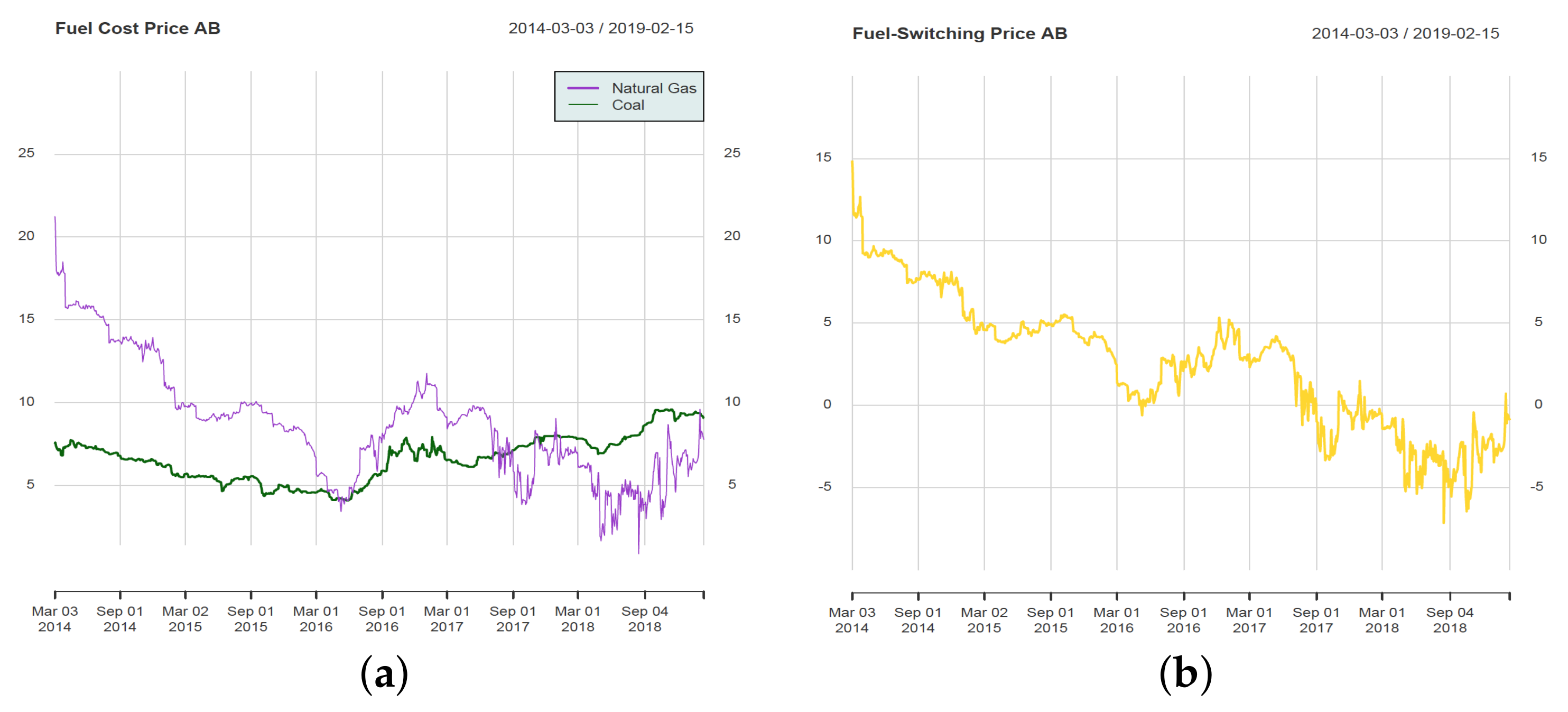
There are many papers that have studied fuel-switching before and there are two main papers we are going to review. First, Goutte and Chevalier 2015 [15] introduced an estimation methodology for Lévy-driven Ornstein–Uhlenbeck processes and applied them on the fuel-switching price in the European market. They also defined a calculation formula to fuel-switching price based on power plants efficiency, fuel price, emissions factor and etc. They mainly concluded that the political decisions impact the jumping nature of the process and enhance our understanding of emission reduction through power systems that could be achieved in the EU Emissions Trading System (EU-ETS). We are going to introduce the fuel-switching price below.

As we discussed before, the fuel-switching price should stimulate companies to reduce GHG in a profitable way. Hence, this price starts from defining the marginal cost of each fuel without a carbon cost:

$$\mathrm{MC}=\frac{\mathrm{FC}}{\eta },$$

(1)

where FC represents fuel cost and $\eta$ is the power plant’s efficiency. In this paper, we do not account for any cost that is related to regulatory cost, maintenance, labour force cost, etc and we follow the same definitions mentioned in Goutte and Chevalier 2015 [15]. Thus, here, the total/average cost for one kWh power generation is equal only to fuel cost. Further, the marginal cost defined here is different from the classic definition of marginal cost which is the change in the total cost that arises when one unit of production is incremented by one. The power plant’s efficiency is considered as an average efficiency, so the marginal cost is actually only affected by the fuel cost. Next, if we have carbon cost such as carbon tax or allowance price, the equation changes to:

$$\mathrm{MC}=\frac{\mathrm{FC}}{\eta }+\frac{\mathrm{EF}}{\eta }\mathrm{EC},$$

(2)

where EF is the emission factor, which depends on the fuel and the amount of fuel burnt, and EC is the emission cost. For simplicity, we do not consider any cost. Now, the fuel switching happens when generated from other fuel is cheaper, so to define the minimum cost for a switch to occur, we need to let ${\mathrm{MC}}_{\mathrm{coal}}={\mathrm{MC}}_{\mathrm{gas}}$, which turns out as solving the emission cost inside this equation:

$${\mathrm{EC}}_{\mathrm{switch}}=\frac{{\eta }_{\mathrm{coal}}{\mathrm{FC}}_{\mathrm{gas}}-{\eta }_{\mathrm{gas}}{\mathrm{FC}}_{\mathrm{coal}}}{{\eta }_{\mathrm{gas}}{\mathrm{EF}}_{\mathrm{coal}}-{\eta }_{\mathrm{coal}}{\mathrm{EF}}_{\mathrm{gas}}}.$$

(3)

Thus, when the EU Allowance price is lower than this price, generating electricity from coal is cheaper than natural gas and vice versa. Later, they used this price in the European market and modelling it by a jump mean reverting model. They conclude that jump modelling techniques should included when modelling fuel-switching price.

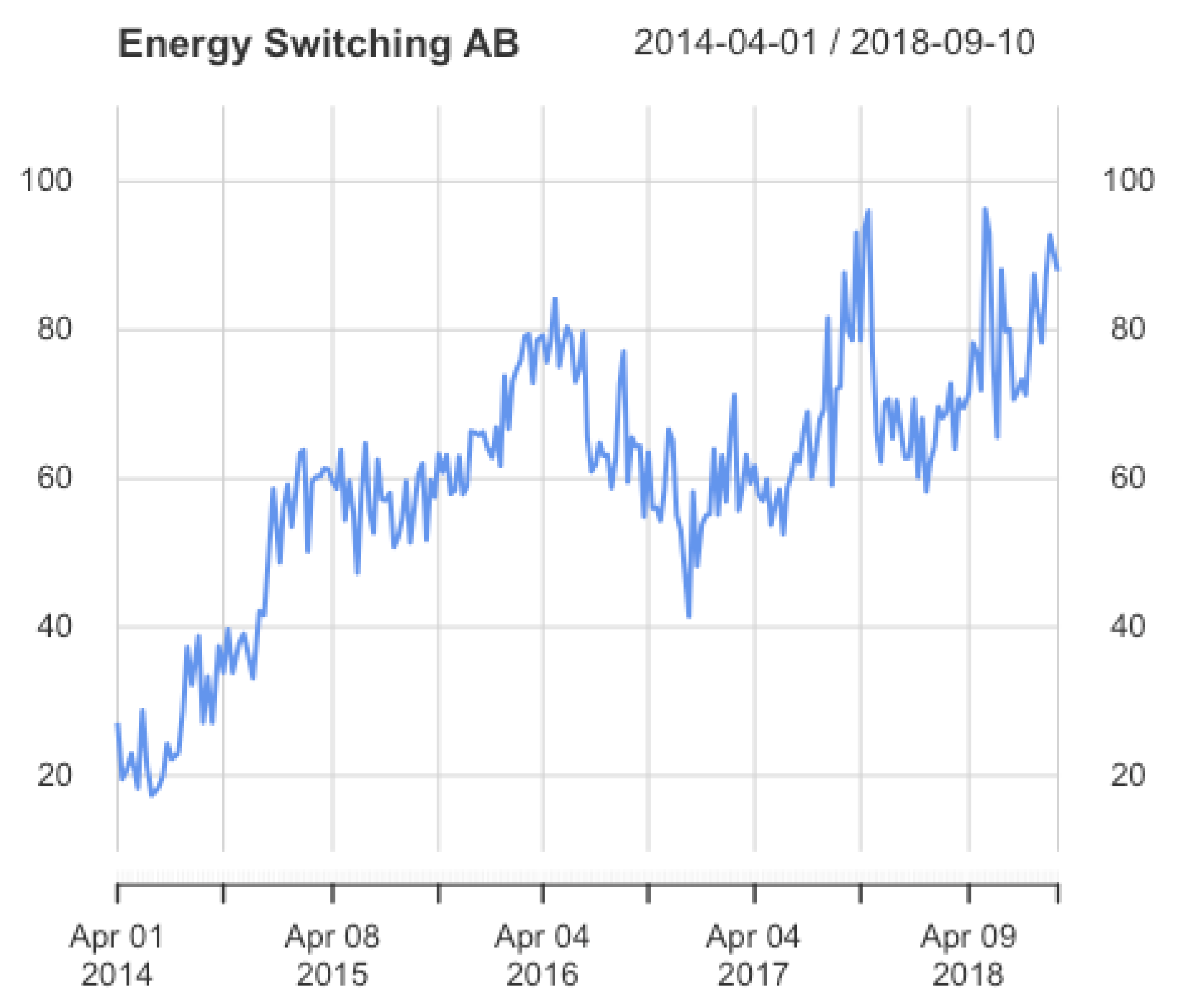
The paper by Arrigoni et al. 2019 [8] introduces this method to the Albertan energy market, and based on the difference situations between the Albertan and European energy markets, they also introduced an energy-switching price as a ‘future’ fuel-switching price which considers a fuel-switching between natural gas and wind. They then also present their ideas as poster in the 42nd International Association for Energy Economics (IAEE) Annual Conference [16]. This is more meaningful because coal to natural gas is a switch to cleaner energy, while natural gas to wind is a switch to renewable energy. Later, similar to Goutte et al., 2015 [15], they modelled these two prices using Levy-driven Ornstein–Uhlenbeck process and standard Ornstein–Uhlenbeck process, and concluded that jump modelling techniques is needed.

The paper by Fargos et al., 2021 [17] offers new insights into the risk of carbon leakage and industrial relocation in case of asymmetric climate policies, and provides an improved understanding of the sectoral and regional structure of leakage, as well as policy measures to mitigate the adverse impacts on industrial competitiveness. Regarding the existing literature, this paper goes beyond it by considering: (1) assessing for the first time the competitiveness impacts of the ambitious EU Green Deal targets towards climate neutrality (no green house gas emission) by mid-century, (2) using an advanced version of the leading GEM-E3-FIT model (which is a multi-regional, multi-sectoral, recursive dynamic computable general equilibrium (CGE) model) with an enhanced representation of energy system and technologies required for net-zero transition. Here net-zero transition is brought out by Global Future Council of the World Economic Forum, which represents reducing global greenhouse gas emissions to ‘net zero’ by 2050, (3) exploring the impacts of first-mover coalitions conceptualizing the most recent climate policy announcements of EU and China aiming to achieve carbon neutrality (i.e., achieving net zero carbon dioxide emissions by balancing carbon dioxide emissions) by mid-century, thus ensuring high policy relevance of the analysis and (4) assessing the cost-effectiveness of border carbon adjustment (BCA) mechanism in preventing carbon leakage and supporting the European Emissions-Intensive and Trade-Exposed (EITE) industries, as suggested by the EU Green Deal.

The paper by Montenegro et al. (2021) [18] reviews the recent literature on the model-based methods utilized for policy analyses in the areas of economics, energy systems, and environmental damages. It also explores ways in which these models and methodologies depict distributional impacts, the main indicators obtained from their results, shortcomings of each modelling methodology, and suggest improvements for future research. Georgescu-Roegen (1971) [19] mentioned that it could generate a reverse or duel case if using the temporal borders of economic process method, that two identical technologies could have two different productivities or marginal cost after several years.

This paper is organized as follows. In Section 2, we introduce the economic background and fuel-switching data used in this paper. Section 3 described the parameters estimation procedures for five stochastic models considered in this paper and introduced in Appendix A. Section 4 gives the empirical results obtained by applying the models from Appendix A to the data introduced in Section 2. Section 5 provides model comparison based on AIC and BIC, and cross-validation methods. The Conclusion is given in Section 6. Appendix A discusses five mean-reverting stochastic models which are used in this paper.

2. Economic Background and the Data

2.1. Economic Content

Signed in 2016, the Pairs Agreement which is an agreement within the United Nations Framework Convention on Climate Change (UNFCC) aimed at dealing with GHG-emissions mitigation, adaptation, and finance. Its goal can be summarized in three parts: (1) Limit the long-term increase of temperature to 1.5 degrees which should be done by reducing emissions as much as possible. (2) Provide a framework for transparency, accountability, and the achievement of more ambitious targets. (3) Mobilize support for climate change mitigation and adaptation. Under this agreement, each country should determine a plan to mitigate warming. According to these, the federal government of Canada published “The pan-Canadian approach to pricing Carbon Pollution” in October 2016 as we mentioned in the beginning and Alberta choose the taxation method for reducing GHG emission. It raises the public’s attention on the carbon pricing method.

The prices in the energy sector mainly depend on two aspects. The electricity prices determine majorly on the prices in the energy market such as coal and gas futures, plus the carbon tax in one of the two forms. These factors are usually affected by the supply and demand in the energy market. Further, the fuel-switching is another important aspect to consider when pricing electricity. Theoretically, the switching can happen between either coal, gas or nuclear, but in practise, switching from coal or gas to nuclear seems difficult since nuclear energy is not flexible. There are several reasons the study of fuel switching is needed. In general, there is a trade-off between coal fire plant and gas fire plant that the coal causes more GHG emissions while gas is more expensive, and this can be applied in the switching. Moreover, the fuel-switching between coal and gas appears to be a natural cost effective way to reduce ${\mathrm{CO}}_2$ emission (Ellerman and Buchner 2007 [20]). At last, a stochastic modelling on fuel-switching gives various applications in operation management and risk management. These reasons make the accurate modelling on fuel switching to become very important.

2.2. The Fuel-Switching Data

We use the fuel-switching and energy-switching price of Alberta as presented in Arrigoni et al. (2019) [8]. We are interested in how these processes are performed on this data and what are the general properties of this data reflected by these processes. Moreover, it would be better if we can study this data using one of the mean reverting models, this is why we introduce a cross validation method in Section 5.

In Arrigoni et al. (2019) [8], the authors provided a new method for carbon pricing based on the European energy market experience which we reviewed in chapter one. Remember that the fuel-switching price is defined as

$${\mathrm{EC}}_{\mathrm{switch}}=\frac{{\eta }_{\mathrm{coal}}{\mathrm{FC}}_{\mathrm{gas}}-{\eta }_{\mathrm{gas}}{\mathrm{FC}}_{\mathrm{coal}}}{{\eta }_{\mathrm{gas}}{\mathrm{EF}}_{\mathrm{coal}}-{\eta }_{\mathrm{coal}}{\mathrm{EF}}_{\mathrm{gas}}}.$$

(4)

To calculate this price, they found the emission factor is equal to 210 kgCO2eq/MWh for natural gas and 320 kgCO2eq/MWh for coal from the financial data of Winnipeg. Further, a case study from JEM Energy in 2004 gives the average coal efficiency which is 32.6%, and 31.1% for natural gas in Albertan power plants. The coal market price and natural gas market price are derived from NRG stream. Thus, one can calculate the fuel-switching price based on the information above, and the data are given in Figure 1.

As we can see from the yellow line in Figure 1, it is negative after September 2017, which means that electricity from natural gas is always more profitable than coal. Hence, it is reasonable to consider a switch between natural gas to wind. So they provide an energy-switching price, where the emission factor for wind is zero and efficiency for wind ranges from 32% to 37%. In the paper, they also generate a wind price by a random uniformly distributed process lies between 37$ to 42.5$. So the energy-switching price is given in Figure Section 2.

We also provide the descriptive statistics for our data in

Table 1. Summary statistics of fuel-switching and energy-switching data.

	Mean	Standard Deviation	Kurtosis	Skewness	Min	Max
fuel-switching	2.553058	3.976492	−0.5539386	0.04961635	−7.15667	14.88465
energy-switching	61.08916	15.98072	0.6200243	−0.7082977	15.60934	95.58245

. As we can see, we have a negative kurtosis and a positive skewness in fuel-switching data which means this data have a thin-tail and are left-skewed. Furthermore, the negative skewness of energy-switching data indicates that the mean of the data values is less than the median, while the positive kurtosis implies a fat tailed distribution.

Although it is hard to see graphically from Figure 1 and Figure 2 that Albertan government had the carbon tax in places in January first 2017, the results from regime switching models reveal some signals of it. In the next section, we are going to give the model estimation result of the fuel-switching price and energy-switching price based on Albertan market by a panel of mean reverting processes we introduced before.

3. Parameter Estimation

3.1. Inhomogeneous Geometric Brownian Motion

Using time changed method, Swishchuk (2008) [10] obtained the solution to the inhomogeneous geometric Brownian motion model (IGBM):

$$d{S}_t=a(L-S_t)dt+\sigma S_{t}d{w}_t,$$

which is

$$S_t=e^{-at}(S_0-L+\tilde{w}\left({\varphi }_t^{-1}\right))+L.$$

where ${\varphi }_t^{-1}={\sigma }^2{\int }_0^t{(S_0-L+\tilde{w}\left({\varphi }_s^{-1}\right)+e^{as}L)}^{2}ds$ and $\tilde{w}\left(t\right)$ is standard Brownian Motion.

In order to fit this model into our data, we consider the calibration of this model using the solution above. Firstly, according to the solution we have

$$\begin{array}{cc}\hfill d{S}_t& =e^{-at}d\tilde{w}\left({\varphi }_t^{-1}\right)-a·e^{-at}[S_0-L+\tilde{w}\left({\varphi }_t^{-1}\right)]dt\hfill \\ & =e^{-at}d\tilde{w}\left({\varphi }_t^{-1}\right)-a·[S_t-L]dt.\hfill \end{array}$$

Then calibrating the above equation we obtain (assuming here we have data set = {$S_{t_1},S_{t_2},S_{t_3},\dots ,S_{t_N}$}):

$$S_{t_{k+1}}-S_{t_k}=e^{-a{t}_k}[\tilde{w}({\varphi }_{t_{k+1}}^{-1})-\tilde{w}({\varphi }_{t_k}^{-1})]-a(S_{t_k}-L)·(t_{k+1}-t_k),$$

which is then equivalent to

$$[S_{t_{k+1}}-S_{t_k}+a(S_{t_k}-L)\Delta t]·e^{a{t}_k}=\tilde{w}({\varphi }_{t_{k+1}}^{-1})-\tilde{w}({\varphi }_{t_k}^{-1})$$

with k = 1, 2, …, N − 1.

Since $\tilde{w}\left(t\right)$ is Standard Brownian Motion and from the properties of it we know that $\tilde{w}({\varphi }_{t_{k+1}}^{-1})-\tilde{w}({\varphi }_{t_k}^{-1})$ is following a normal distribution with mean 0 and variance $Var[\tilde{w}({\varphi }_{t_{k+1}}^{-1})-\tilde{w}({\varphi }_{t_k}^{-1})]$.

Now since ${\varphi }_t^{-1}={\sigma }^2{\int }_0^t{(S_0-L+\tilde{w}({\varphi }_s^{-1})+e^{as}L)}^{2}ds$ is an increasing function with respect to t, we have ${\varphi }_{t_{k+1}}^{-1}>{\varphi }_{t_k}^{-1}$, so then

$$\begin{array}{cc}\hfill Var[\tilde{w}({\varphi }_{t_{k+1}}^{-1})-\tilde{w}({\varphi }_{t_k}^{-1})]& =E[{\tilde{w}}^2({\varphi }_{t_{k+1}}^{-1})]-E[{\tilde{w}}^2({\varphi }_{t_k}^{-1})]\hfill \\ & ={\sigma }^2[{(S_0-L)}^2\frac{e^{{\sigma }^2{t}_{k+1}}-e^{{\sigma }^2{t}_k}}{{\sigma }^2}+\frac{L^2(e^{2a{t}_{k+1}}-e^{2a{t}_k}+e^{{\sigma }^2{t}_k}-e^{{\sigma }^2{t}_{k+1}})}{2a-{\sigma }^2}\hfill \\ & +\frac{2L(S_0-L)(e^{a{t}_{k+1}}-e^{a{t}_k}+e^{{\sigma }^2{t}_k}-e^{{\sigma }^2{t}_{k+1}})}{a-{\sigma }^2}].\hfill \end{array}$$

Thus, the log-likelihood for $X_{t_k}=[S_{t_{k+1}}-S_{t_k}+a(S_{t_k}-L)\Delta t]·e^{a{t}_k}$ is given by:

$$l(X_t;a,L,\sigma )=-\sum _{k=1}^{n-1}\frac{1}{2}log\left(2\pi V_k^2\right)-\sum _{k=1}^{n-1}\frac{{[S_{t_{k+1}}-S_{t_k}+a(S_{t_k}-L)\Delta t]}^2·e^{2a{t}_k}}{2V_k^2},$$

where n is the length of $S_t$ and $V_k=Var[\tilde{w}({\varphi }_{t_{k+1}}^{-1})-\tilde{w}({\varphi }_{t_k}^{-1})]$.

As we can see from the above formula of $Var[\tilde{w}({\varphi }_{t_{k+1}}^{-1})-\tilde{w}({\varphi }_{t_k}^{-1})]$, it contains many exponential terms. Take $e^{a{t}_k}$ as an example, if $a{t}_k$ is greater than 708, then R cannot compute such big value and thus it will print Inf. So the algorithm for calculating maximized likelihood estimator is very sensitive to the initial value. Based on this, we choose to use the result from as our initial value and we set time scale as $0,\frac{1}{n},\frac{2}{n},\dots ,\frac{n-1}{n}$ to compensate this defect, where n is the length of our data.

Now in order to maximize the log-likelihood and let our algorithm search in a correct parameter space, we need to maximize the log-likelihood under several constrains for our parameters:

$$Var[\tilde{w}({\varphi }_{t_{k+1}}^{-1})-\tilde{w}({\varphi }_{t_k}^{-1})]>0forallk=1,\dots ,n-1;$$

$$|a-{\sigma }^2|>0(i.e.,a\ne {\sigma }^2);$$

$$|2a-{\sigma }^2|>0(i.e.,2a\ne {\sigma }^2);$$

$$-708<2a{t}_n<708;$$

$$0<{\sigma }^2{t}_n<708.$$

In the later section, we will proceed to a Augmented Lagrangian Adaptive Barrier Algorithm to find our maximum likelihood estimator.

3.2. OU Process and Lévy-Driven OU Process

3.2.1. Parameter Estimation

We are going to present a two steps estimation procedure introduced by Goutte and Chevalier (2015) [15]. Firstly, we use the Ordinary Least Square (OLS) method to estimate parameters $\kappa$, $\theta$ and $\sigma$ in OU process. Secondly, the Maximized Likelihood Estimation will be used to model the parameters in Lévy NIG distribution.

In the previous section we have the solution to OU process and LDOU process which is

$$S_{t_{k+1}}=S_{t_k}{e}^{-\kappa \Delta t}+\theta (1-e^{-\kappa \Delta t})+{\int }_{t_k}^{t_{k+1}}{e}^{\kappa (s-t_{k+1})}\sigma d{Y}_s.$$

(5)

where $Y_t=W_t$ for OU process, $Y_t=L_t$ for LDOU process and $\Delta t=t_{k+1}-t_k$. Here we change the time interval from $[0,t]$ to $[t_k,t_{k+1}]$ because in practice, we observed the data in time increments $0<t_0<t_1<\dots <t_n$ with $\Delta t=t_{k+1}-t_k$ be a constant. Now rearrange this equation we obtain:

$$S_{t_{k+1}}-S_{t_k}=m-a{S}_{t_k}+v{ϵ}_{t_k},$$

(6)

where $m=(1-e^{-\kappa \Delta t})\theta$, $a=1-e^{-\kappa \Delta t}$, $v=\sqrt{\frac{1-e^{-2\kappa \Delta t}}{2\kappa }}\sigma$ and ${ϵ}_{t_k}=\frac{1}{s}{\int }_{t_k}^{t_{k+1}}{e}^{\kappa (s-t_{k+1})}\sigma d{Y}_s.$

Notice that the term $v{ϵ}_{t_k}$ is a white noise, where white noise means it has zero mean with constant finite variance, and no autocorrelation or autocovariance. We consider the Ordinary Least Square (OLS) method for Equation (6) which is one of the popular parameter estimation methods for an autoregressive model of order one (AR(1)), then our first step to estimate parameter $\{\kappa ,\theta ,\sigma \}$ is to minimize the empirical variance of white noise:

$$\widehat{Var}\left(v{ϵ}_{t_k}\right)=\frac{1}{n}\sum _{k=0}^{n-1}{(S_{t_{k+1}}-S_{t_k}-m+a{S}_{t_k})}^2$$

The solution is given by:

$$\left(\begin{array}{c}\widehat{m}\\ 1-\widehat{a}\end{array}\right)={\left(A^{\prime }A\right)}^{-1}{A}^{\prime }B$$

(7)

where $A=\left(\begin{array}{cc}1& S_{n-1}\\ \dots & \dots \\ 1& S_0\end{array}\right)$ and $B=\left(\begin{array}{c}{S}_n\\ \dots \\ S_1\end{array}\right)$ and $v^2$ is estimated by

$${\widehat{v}}^2=\frac{1}{n}\sum _{k=0}^{n-1}{(S_{t_{k+1}}-S_{t_k}-\widehat{m}+\widehat{a}{S}_{t_k})}^2$$

(8)

Suppose the $Y_t$ inside term ${ϵ}_{t_k}$ is a Wiener process (corresponding to OU process), then till now we already find out the estimators of parameters in OU process. However, when $Y_t$ is a Levy process with NIG distribution, we need our second step to estimate parameters $\{\alpha ,\beta ,\delta ,\mu \}$ for NIG. Noticing that in LDOU case, $S_{t_{k+1}}-S_{t_k}+a{S}_{t_k}=m+v{ϵ}_{t_k}$ is following a non-centered and un-normalized NIG distribution, so we are considering the MLE method for these four parameters. By Barndorff-Nielsen and Halgreen (1977) [21], they have proved the log-likelihood function of $NIG(\alpha ,\beta ,\delta ,\mu )$ distribution for a set of i.i.d random variables $x_1,\dots ,x_n$ is

$$L(x_i;\alpha ,\beta ,\delta ,\mu )=nlog\frac{\alpha }{\pi }+n\delta \gamma +\sum _{\begin{array}{c}k=0\end{array}}^{n-1}[\beta \delta {\tau }_k-log{a}_k+log{K}_1\left(\alpha \delta a_k\right)]$$

(9)

where ${\tau }_k=\frac{x_k-\mu }{\delta }$, $a_k=\sqrt{1+{\tau }_k^2}$ and $K_1$ is the same function in the density of NIG.

Thus, if we let $x_k=S_{t_{k+1}}-S_{t_k}+\widehat{a}{S}_{t_k}$ in Equation (9), the only thing we need to do next is to maximize function (9) with respect to parameters $(\alpha ,\beta ,\delta ,\mu )$. However, since the log-likelihood function is very complicated, we consider using the $nigFit$ function in R package “GeneralizedHyperbolic” to find the MLE, which use a numeric way to maximize this function. Moreover, notice that in definition of NIG distribution, we need $\delta >0$, $\alpha \ge 0$ and $\gamma \ge 0$, so we are going to maximize the log-likelihood under constrains.

3.2.2. Parameters Initialization

Since we are going to maximize this function numerically, we have to decide the initial value for the algorithm. Here we consider a method of moments for our initial value. In Jordan S. (1999) [22], he present the formula for the first four moments of NIG distribution:

$$m_1\approx E\left[x\right]=\mu +\delta \beta {\gamma }^{-1}$$

(10)

$$m_2\approx E\left[x^2\right]=\delta {\alpha }^2{\gamma }^{-3}$$

(11)

$$m_3\approx E\left[x^3\right]=3\delta \beta {\alpha }^2{\gamma }^{-5}$$

(12)

$$m_4\approx E\left[x^4\right]=3\delta \beta {\alpha }^2({\alpha }^2+4{\beta }^2){\gamma }^{-7}$$

(13)

where $m_i$ is the sample moments of i.i.d random variables $x_i$ which follow $NIG(\alpha ,\beta ,\delta ,\mu )$ distribution and $\gamma =\sqrt{{\alpha }^2-{\beta }^2}$. Then solving the parameters from Equations (10) to (13), we obtain our formula of initial values.

$$\begin{array}{cc}\hfill {\gamma }_0& =\frac{3}{\overline{S}\sqrt{3{\overline{\gamma }}_2-5{\overline{\gamma }}_1}}\hfill \end{array}$$

(14)

$$\begin{array}{cc}\hfill {\beta }_0& =\frac{{\overline{\gamma }}_1\overline{S}{\gamma }_0^2}{3}\hfill \end{array}$$

(15)

$$\begin{array}{cc}\hfill {\delta }_0& =\frac{{\overline{S}}^2{\gamma }_0^3}{{\beta }_0^2+{\gamma }_0^2}\hfill \end{array}$$

(16)

$$\begin{array}{cc}\hfill {\mu }_0& =\overline{X}-{\beta }_0\frac{{\delta }_0}{\gamma }\hfill \end{array}$$

(17)

where $\overline{X}=\frac{1}{n}{\sum }_{\begin{array}{c}i=1\end{array}}^n{x}_i$, $\overline{S}=\frac{1}{n}{\sum }_{\begin{array}{c}i=1\end{array}}^n{(x_i-\overline{X})}^2$, ${\overline{\gamma }}_1=\frac{{\mu }_3}{{\mu }_2^{3/2}}$ and ${\overline{\gamma }}_2=\frac{{\mu }_4}{{\mu }_2^2}-2$ with ${\mu }_k=\frac{1}{n}{\sum }_{\begin{array}{c}i=1\end{array}}^n{(x_i-\overline{x})}^k$.

These result can also be found in Goutte and Chevalier (2015) [15].

3.3. Regime-Switching Models

In the application below, we are going to consider a two-state continuous-time Markov Chain $Z_t$ and these two states represent the ‘expansion’ and ‘contraction’ in economics. The transition of this Markov chain determined the probability that of our parameters will switch to another regime. Considering the complicated form of SDE of these two processes, we are not going to find their explicit solution. Instead, we will use EM algorithm to estimate parameters in it. Moreover, these processes also have the mean-reverting properties while under different states, it will have a different long-term mean, mean reverting rate, volatility, and even the parameters in Lévy process.

3.3.1. Parameter Estimation of RSOU Models Using EM Algorithm

Recall that the RSOU and RSLDOU are the solution to the SDE

$$d{X}_t=\kappa \left(Z_t\right)(\theta \left(Z_t\right)-X_t)dt+\sigma \left(Z_t\right)d{Y}_t$$

(18)

where $Y_t$ can be Wiener process or Levy process. Since it is complicate to find a explicit solution when we add a Markov chain in it, we discretize these two processes by their SDE. For the observed price $\{S_{t_1},S_{t_2},\dots ,S_{t_n}\}$, we have:

$$S_{t_{k+1}}=S_{t_k}+\kappa \left(Z_{t_k}\right)(\theta \left(Z_{t_k}\right)-S_{t_k}){\Delta }_t+\sigma \left(Z_{t_k}\right){ϵ}_{t_k}$$

(19)

We use the EM algorithm estimation procedure which was introduced in Julien Chevallier and Stéphane Goutte (2016) [23] to estimate parameters in RSOU process: ${\Theta }_1:=\{\kappa \left(Z_t\right),\theta \left(Z_t\right),\sigma \left(Z_t\right)\}$. For simplicity, we will write $S_{t_k}$, $Z_{t_k}$, $\kappa (Z_{t_k}=i)$, $\theta (Z_{t_k}=i)$ and $\sigma (Z_{t_k}=i)$ as $S_k$, $Z_k$, ${\kappa }_i$, ${\theta }_i$ and ${\sigma }_i$ in the following formula.

For the expectation step, they first calculate the filtered probability:

$$P(Z_k=i|{\mathcal{F}}_k^S;{\widehat{\Theta }}_1^{\left(m\right)})=\frac{P(Z_k=i|{\mathcal{F}}_{k-1}^S;{\widehat{\Theta }}_1^{\left(m\right)})f(S_k|Z_k=i;{\mathcal{F}}_{k-1}^S;{\widehat{\Theta }}_1^{\left(m\right)})}{\sum _{j\in S}P(Z_k=j|{\mathcal{F}}_{k-1}^S;{\widehat{\Theta }}_1^{\left(m\right)})f(S_k|Z_k=j;{\mathcal{F}}_{k-1}^S;{\widehat{\Theta }}_1^{\left(m\right)})}$$

(20)

where

$$P(Z_k=i|{\mathcal{F}}_{k-1}^S;{\widehat{\Theta }}_1^{\left(m\right)})=\sum _{j\in S}{\Pi }_{ij}^{\left(n\right)}P(Z_{k-1}=i|{\mathcal{F}}_{k-1}^S;{\widehat{\Theta }}_1^{\left(m\right)})$$

(21)

and

$$f(S_k|Z_k=i;{\mathcal{F}}_{k-1}^S;{\widehat{\Theta }}_1^{\left(m\right)})=\frac{1}{\sqrt{2\pi }{\sigma }_i^{\left(m\right)}}\exp \left\{-\frac{{(S_k-{\kappa }_i^{\left(m\right)}{\theta }_i^{\left(m\right)}-(1-{\kappa }_i^{\left(m\right)})S_{k-1})}^2}{2{({\sigma }_i^{\left(m\right)})}^2}\right\}$$

(22)

because of the Wiener process term in RSOU process. Then they calculate the Smoothed probability,

$$P(Z_k=i|{\mathcal{F}}_N^S;{\widehat{\Theta }}_1^{\left(m\right)})=\sum _{j\in S}\left\{\frac{P(Z_k=i|{\mathcal{F}}_k^S;{\widehat{\Theta }}_1^{\left(m\right)})P(Z_{k+1}=j|{\mathcal{F}}_N^S;{\widehat{\Theta }}_1^{\left(m\right)}){\Pi }_{ij}^{\left(n\right)}}{P(Z_{k+1}=i|{\mathcal{F}}_k^S;{\widehat{\Theta }}_1^{\left(m\right)})}\right\}$$

(23)

At last, for the maximize step, they provided a iterative solution which is given by:

$${\theta }_i^{(m+1)}=\frac{\sum _{k=2}^{N}P(Z_k=i|{\mathcal{F}}_N;{\widehat{\Theta }}_1^{\left(m\right)})(S_k-(1-{\kappa }_I^{(m+1)})S_{k-1})}{{\kappa }_i^{(m+1)}\sum _{k=2}^{N}P(Z_k=i|{\mathcal{F}}_N;{\widehat{\Theta }}_1^{\left(m\right)})}$$

(24)

$${\kappa }_i^{(m+1)}=\frac{\sum _{k=2}^{N}P(Z_k=i|{\mathcal{F}}_N;{\widehat{\Theta }}_1^{\left(m\right)})S_{k-1}{B}_1}{\sum _{k=2}^{N}P(Z_k=i|{\mathcal{F}}_N;{\widehat{\Theta }}_1^{\left(m\right)})S_{k-1}{B}_2}$$

(25)

$${\sigma }_i^{2(m+1)}=\frac{\sum _{k=2}^{N}P(Z_k=i|{\mathcal{F}}_N;{\widehat{\Theta }}_1^{\left(m\right)}){(S_k-{\kappa }_i^{(m+1)}{\theta }_i^{(m+1)}-(1-{\kappa }_i^{(m+1)})S_{k-1})}^2}{\sum _{k=2}^{N}P(Z_k=i|{\mathcal{F}}_N;{\widehat{\Theta }}_1^{\left(m\right)})}$$

(26)

$${\Pi }_{ij}^{(m+1)}=\frac{\sum _{k=2}^{N}P(Z_k=j|{\mathcal{F}}_N^S;{\widehat{\Theta }}_1^{\left(m\right)})\frac{{\Pi }_{ij}^{\left(m\right)}P(Z_{k-1}=i|{\mathcal{F}}_{k-1}^S;{\widehat{\Theta }}_1^{\left(m\right)})}{P(Z_k=j|{\mathcal{F}}_{k-1}^S;{\widehat{\Theta }}_1^{\left(m\right)})}}{\sum _{k=2}^{N}P(Z_k=i|{\mathcal{F}}_N^S;{\widehat{\Theta }}_1^{\left(m\right)})}$$

(27)

where

$$B_1=S_k-S_{k-1}-\frac{\sum _{k=2}^{N}P(Z_k=i|{\mathcal{F}}_N^S;{\widehat{\Theta }}_1^{\left(m\right)})(S_k-S_{k-1})}{\sum _{k=2}^{N}P(Z_k=i|{\mathcal{F}}_N^S;{\widehat{\Theta }}_1^{\left(m\right)})},$$

(28)

$$B_2=\frac{\sum _{k=2}^{N}P(Z_k=i|{\mathcal{F}}_N^S;{\widehat{\Theta }}_1^{\left(m\right)})S_{k-1}}{\sum _{k=2}^{N}P(Z_k=i|{\mathcal{F}}_N^S;{\widehat{\Theta }}_1^{\left(m\right)})}-S_{k-1}.$$

(29)

In our cases, we only consider a two-states Markov chain, which means our stats space $S=\{1,2\}$. The next step of this algorithm is to set an ending constraint for it. Since we are aiming at maximize the log-likelihood, so one of the constrain is $\log L^{(m+1)}-\log L^{\left(m\right)}<ϵ$. Another constrain we set is that $m<M$ where M is a fixed number of iterations we want, since this algorithm might converge very slowly.

3.3.2. Parameter Estimation of the NIG Part of RSLDOU Model Using MLE Algorithm

After estimate the parameters ${\Theta }_1$, we then proceed to the remaining set of parameters ${\Theta }_2$ in NIG distribution. Recall that in Section 3.2.1, we talked about how to estimate NIG parameters using MLE method, here we are using the similar technique instead of that we have two regimes now. Thus, to estimate the remaining set of parameters, we fit NIG distributions for each regime:

$$S\left(Regime1\right)\sim L_1({\alpha }_1,{\beta }_1,{\delta }_1,{\mu }_1)$$

(30)

and

$$S\left(Regime2\right)\sim L_2({\alpha }_2,{\beta }_2,{\delta }_2,{\mu }_2).$$

(31)

Following the same procedures in Section 3.1, we can obtain the estimates ${\widehat{\Theta }}_2=\{\widehat{{\alpha }_1},\widehat{{\beta }_1},\widehat{{\delta }_1},\widehat{{\mu }_1},\widehat{{\alpha }_2},\widehat{{\beta }_2},\widehat{{\delta }_2},\widehat{{\mu }_2}\}$.

4. Empirical Results

4.1. Estimation Results for Fuel-Switching Data

4.1.1. Estimation of IGBM

When it comes to change of time approach, as we have talked before, due to the limits of exponential term in computer, the algorithm is quite sensitive to the initial values. Thus, in this problem, we use the estimators in Euler-scheme calibration method to be our initial value and Augmented Lagrangian Adaptive Barrier Algorithm to find our maximum likelihood estimator. The results are shown in

Table 2. Estimation result of IGBM for fuel-switching data.

a	L	$\mathit{\sigma }$
$\times {2.514925}^{-12}$	−2.212315	0.02235206

.

One of the simulation results in given by Figure 3.

The reason we have this terrible result is because IGBM keeps the simulation positive all the time. So this model is typically not fit for our fuel switching data since the data decrease below 0 at the end. Thus, we do not consider this situation in the later model comparison section.

4.1.2. Estimation of OU and LDOU Processes

Table 3. Estimation Result of OU and LDOU model on fuel-switching data.

$\mathit{\kappa }$	$\mathit{\theta }$	$\mathit{\sigma }$	$\mathit{\alpha }$	$\mathit{\beta }$	$\mathit{\delta }$	$\mathit{\mu }$
0.008600791	1.10466	0.4005829	0.2418017	−0.05377233	0.2637261	0.06009332

gives esitmation result of OU and LDOU model and Figure 4 present our simulation result.

In Table 3, the $\theta$ is 1.10466 which represents a very low long-term mean and we also have a very small mean-reverting rate $\kappa =0.008600791$. The $\alpha$ in NIG is close to 0 witch indicates a high intensity of jumps in Lévy process. Comparing to Figure 3, the simulation result of OU process present in Figure 4 is clearly better, since OU process allows negative values. However, we might also see that it reaches negative value in a very early date and bounce back to positive, which could be a signal for not fitting the data well.

Figure 4 also gives simulation results for the LDOU process, we can see there are lots of ‘cliffs’ inside the process, which is the consequence of introducing Lévy process to the model. Next, we talk about the solution of regime-switching models on fuel-switching price.

4.1.3. Estimation of RSOU and RSLDOU Processes

The estimation result for regime switching OU process is given by

Table 4. Estimation result of RSOU for fuel-switching data.

${\mathit{\kappa }}_1$	${\mathit{\kappa }}_2$	${\mathit{\theta }}_1$	${\mathit{\theta }}_2$	${\mathit{\sigma }}_1^2$	${\mathit{\sigma }}_2^2$	${\mathit{\pi }}_{11}$	${\mathit{\pi }}_{22}$
0.00310	0.03306	4.9722	−1.7579	0.01146	0.4887	0.9370	0.8528

. In Table 4, we can see that regime 1 has a positive long-term mean while regime 2 has a negative value, and we will also see in the later that this process switch to regime 2 more frequently when time increase. Compare to the volatility in OU process, regime switching model provides a lower and a higher volatility according to different state. Now, one of the simulation result is in Figure 5.

The reason we observe ‘cliffs’ in the trajectory even if we do not include Lévy process is because when each regime changes, this process change its parameters, which cause the ’cliffs’ in the process. Regime switching Lévy driven OU model has the same estimator value as above, but with different estimator for the parameters in NIG distribution. Next, we present the estimators for two NIG distributions according to the two regimes we set before:

The $\alpha$ is increasing in regime two means a lower intensity of jump happened in Lévy process in regime two. Further we have a negative beta value which implies a left skew in NIG distribution. One of the simulation result is present in Figure 6:

To see when the switching happened in our simulation result, we need to have a closer look at the filtered and smoothed probabilities in the regime switching model given in Figure 7.

Figure 7 basically shows the probability of each regime happened in time t. Based on the two graphs, when the number of trials is less than around 850, regime one is more likely to happened and when the number of trials is greater than around 850, it has more possibilities to switch to regime 2. According to our data, a number of trials around 850 is consistent with July in 2017 which is the time Carbon Levy is introduce to Albertan energy market. It tells us that the introduce of carbon tax changes the structure of our data and according to Figure 1, the natural gas will be more profitable for generating electricity after the introduction of carbon tax. Further, from Table 4 and

Table 5. Estimation result of the NIG part of RSLDOU model for fuel-switching data.

${\mathit{\alpha }}_1$	${\mathit{\beta }}_1$	${\mathit{\delta }}_1$	${\mathit{\mu }}_1$
0.5565004	−0.07445405	0.1021734	0.009274105
${\mathit{\alpha }}_{\mathbf{2}}$	${\mathit{\beta }}_{\mathbf{2}}$	${\mathit{\delta }}_{\mathbf{2}}$	${\mathit{\mu }}_{\mathbf{2}}$
1.026705	−0.4044685	0.1459743	0.1332535

, the regime two has greater volatility and higher alpha, which implies a higher volatility and intensity of jumps of fuel-switching data caused by the introduction of carbon levy.

So far, we can see that the regime-switching models provides a better fit graphically compare to OU and LDOU process, since their simulation result have more points close to the original trajectory.

4.2. Estimation Results for Energy-Switching Data

In this section, we follow the same procedure of Section 4.1 and create estimation result of different models for energy-switching data.

4.2.1. Estimation of IGBM

The obtained estimation results for IGBM model are given in

Table 6. Estimates of IGBM model on energy-switching data.

a	L	$\mathit{\sigma }$
0.001173194	100.2216	0.1184857

:

The long-term mean reaches 100 means that this price will go higher in the future to around 100.2216 indicated by the IGBM model. One of the simulation results in given by Figure 8.

We can see that the blue curve do not fit the red curve very well, as it separate with the red curve in the early date and has an intend to go beyond red curve after the final date of this data. Thus, this model may not fit the data very well.

4.2.2. Estimation of OU and LDOU Processes

Table 7. Estimation Result of OU and LDOU model on energy-switching data.

$\mathit{\kappa }$	$\mathit{\theta }$	$\mathit{\sigma }$	$\mathit{\alpha }$	$\mathit{\beta }$	$\mathit{\delta }$	$\mathit{\mu }$
0.08757514	64.3041	6.655671	1.494409	−0.005857812	1.502579	0.005655803

presents the estimation result for OU and LDOU process based on two-step estimation method.

Table 7 give a long-run mean 64.3041 which is smaller than the long-term mean in IGBM model. Further, it has a larger $\alpha$ compares to fuel-switching data which shows that the energy-switching price may includes less jumps compare to the fuel-switching price. Similar as fuel-switching data, we have a negative beta here, which indicates a left skewed density. Figure 9 is the simulation result of OU model. Compare to Figure 8, the blue trajectory goes up and down around the red one and it also perfectly explains the trend of red curve.

So then we are interested in how LDOU model perform on energy-switching data, as we can see from Figure 10, it keeps following the trend of red curve while it has some extreme values in the early dates.

4.2.3. Estimation of RSOU and RSLDOU Processes

The estimation result for regime switching OU process is given by

Table 8. Estimation Result of RSOU model on energy-switching data.

${\mathit{\kappa }}_1$	${\mathit{\kappa }}_2$	${\mathit{\theta }}_1$	${\mathit{\theta }}_2$	${\mathit{\sigma }}_1^2$	${\mathit{\sigma }}_2^2$	${\mathit{\pi }}_{11}$	${\mathit{\pi }}_{22}$
0.075023	1.0327	62.3686	77.8781	25.8930	109.0701	0.9888	0.9209

.

And one of the simulation result is in Figure 11.

Similar as before, Regime Switching Lévy Driven OU model has the same estimator value as above, but with different estimator for the parameters in NIG distribution. So in the next, we only present the estimators for two NIG distributions according to the two regimes we set before in

Table 9. Estimation result of the NIG part of RSLDOU model for energy-switching data.

${\mathit{\alpha }}_1$	${\mathit{\beta }}_1$	${\mathit{\delta }}_1$	${\mathit{\mu }}_1$
0.1550563	0.002312699	7.641092	4.604966
${\mathit{\alpha }}_{\mathbf{2}}$	${\mathit{\beta }}_{\mathbf{2}}$	${\mathit{\delta }}_{\mathbf{2}}$	${\mathit{\mu }}_{\mathbf{2}}$
0.07798173	−0.006995654	9.699337	40.40929

.

Further, we have the simulation result given by Figure 12.

To see the probabilities of regime one and two happened in time t, we report the smoothed and filtered probabilities for energy-switching data in Figure 13.

We can see the switch happened more frequently after the number of trials reaches 170 which is as well the July of 2017 in Figure 2. This indicates that for RSOU model, the volatility and long-term mean are all changes after the introduction of carbon tax in Albertan energy market. Since the volatility for regime two is 109.0701 according to Table 8, and regime one only have ${\sigma }^2=25.8930$, it can say that introduction of carbon tax cause a higher volatility for our energy-switching data. As for the NIG distribution in RSLDOU model, a smaller alpha in regime two means the decrease of steepness or pointiness of the density, which implies a fat tail after July 2017.

If we have a closer look at Figure 4, Figure 5, Figure 6, Figure 7, Figure 8, Figure 9, Figure 10 and Figure 11, it is hard to tell which model fits the data well graphically. Hence, in the next section we are going to propose two model comparison test and hoping to sifting the best fitted model for the two prices.

5. Models Comparison

So far we have fitted the fuel-switching data into five different mean-reverting models: The Inhomogeneous Geometric Brownian Motion (IGBM), OU process, Levy-driven OU process, regime switching OU process and regime switching Levy driven OU process. In this section, we numerically compare their performance on the fuel-switching and energy-switching data.

5.1. AIC and BIC

To compare the goodness of fit of all the models, we first use the Akaike information criteria (AIC) and Bayesian Information Criteria (BIC), as these two criteria are estimators of relative quality of statistical models for a given set of data:

$$\begin{array}{c}\hfill AIC=-2In(\widehat{L})+2kBIC=-2In(\widehat{L})+kIn\left(n\right)\end{array}$$

where $\widehat{L}$ is the likelihood value under Maximum likelihood estimator, k is the number of parameters that need to estimated and n is the number of observation. The smaller of AIC and BIC, the better the model is.

Table 10. Model comparison for fuel-switching data using AIC and BIC, where $5\times {10}^{-324}$ represents the smallest positive double in R.

	Likelihood-Value	AIC	BIC
OU process	<$5\times {10}^{-324}$	3613.942	3629.387
Levy-driven OU process	<$5\times {10}^{-324}$	2414.07	2450.108
regime switching OU process	$5.36326\times {10}^{139}$	−623.4778	−571.9943
regime switching Levy driven OU process	$2.500369\times {10}^{18}$	−48.72594	43.94428

gives the results for fuel-switching data:

As we can see from Table 10, if we only compare the result of OU process and LDOU process, the introduction of jump modeling techniques did create a better model and this result in consistent with the result in Arrigoni et al. (2019) [8]. However, we can see the value of AIC and BIC decrease significantly after we introduce regime-switching model to the data and the RSOU process gives the best fit to the fuel-switching data. Notice that here we do not consider AIC and BIC for IGBM because this model is typically not fit for fuel-switching data, since IGBM is always positive while the data have negative values.

Table 11. Model comparison for energy-switching data using AIC and BIC, where $5\times {10}^{-324}$ represents the smallest positive double in R.

	Likelihood-Value	AIC	BIC
Inhomogeneous Geometric Brownian Motion	<$5\times {10}^{-324}$	1598.655	1608.877
OU process	$9.50999\times {10}^{-138}$	637.0088	647.2303
Levy-driven OU process	$5.098482\times {10}^{-138}$	646.2556	670.1058
regime switching OU process	$5.287361\times {10}^{-314}$	1462.693	1496.765
regime switching Levy driven OU process	$5.41323\times {10}^{-319}$	1501.672	1563.001

gives the comparison results for energy-switching data:

In Table 11, the OU process and LDOU process produced a relatively low value of AIC and BIC, while other models have the value around 1500. It is reasonable since the wind prices used in Arrigoni et al. (2019) [8] is a random uniformly distributed process and the OU process reflect this property.

As we can see from Table 10, our AIC and BIC report negative values, which is reasonable since our data create a relatively large density and cause the $In(\widehat{L})$ to be a positive value. Moreover, this negative value also just depend on the model and have nothing to do with the initial value. If we try a 3-states MC in RSOU or RSLDOU model, we will still obtain negative AIC and BIC. Another worth noticing feature is that the AIC and BIC values are relatively large, this situation also happened in Chevallier and Goutte (2016) [23] and there is no need to re-scale them.

The AIC and BIC give us a general idea of the goodness of fit for each model on the data. In addition, to access the predictability of each model on the data, we propose a cross validation test in the next section. More importantly, in the cross validation test we estimate the mean square error of each model, which is a different comparison scale with respect to AIC and BIC.

5.2. Cross Validation (CV) for Time Series Data: The h-Block Cross Validation

The traditional k-fold cross validation introduced by P. A. Lachenbruch and M. R. Mickey (1968) [24] is a popular method in evaluate machine learning models. The first step of this method is to shuffle the data randomly, while it is impossible for time series data since they already have an order based on time. For times series data, people usually consider a leave-one-out cross validation. Suppose the model we have is

$$x_t=g(\theta ,x_{t-1})$$

(32)

where $\theta$ is a set of parameters in the model and g is a linear function of variable $x_{t-1}$ depend on the model, for example, $g(\theta ,x_{t-1})=\delta +\varphi x_{t-1}+ϵ$ for an AR(1) model. The leave-one-out CV first estimate parameter on the data that removed a single case $x_i$, which we name this set of estimator ${\widehat{\theta }}_i$. Then it assess the predictive ability of the model by the expectation

$$E[{({\tilde{x}}_{i+1}-g(\widehat{\theta },{\tilde{x}}_i))}^2]\approx \frac{1}{n}\sum _{i=1}^n{(x_{i+1}-g({\widehat{\theta }}_1,x_i))}^2.$$

(33)

where ${\tilde{x}}_i$ is a random variable that has same distribution as $x_i$ and $\widehat{\theta }$ is the estimates of original model. However, when $x_t$ are not independent of each other, the estimation of $E[{({\tilde{x}}_{i+1}-g(\widehat{\theta },{\tilde{x}}_i))}^2]$ in Equation (A16) can be very poor. Thus, in the h-block CV [25], instead of removing one case for the i-th parameter estimate, we remove as well a block of h cases from either side of it and then calculate the corrected h-block cross-validated estimate as:

$$E[{({\tilde{x}}_{i+1}-g(\widehat{\theta },{\tilde{x}}_i))}^2]\approx \frac{1}{n}\sum _{i=1}^n{(x_{i+1}-g({\widehat{\theta }}_i,x_i))}^2-\frac{1}{n^2}\sum _{i=1}^n\sum _{j=1}^n{(x_{j+1}-g({\widehat{\theta }}_i,x_j))}^2+\frac{1}{n}{(x_{i+1}-g(\widehat{\theta },x_i))}^2.$$

(34)

Now we use the method given in Equation (A17), which we set h = 2 to make sure the Independence of each test value on our models and produce the following result in

Table 12. The h-block cross-validation result for each model on both prices.

	Fuel-Switching Data	Energy-Switching Data
Inhomogeneous Geometric Brownian Motion		96.95243
OU process	0.1973981	88.33951
Levy-driven OU process	0.1896627	125.8895
regime switching OU process	0.06602948	106.7323
regime switching Levy driven OU process	0.2099495	95.20393

. Similarly as before, we do not test IGBM for fuel-switching data due to inconsistent property between them. Further we are happy to see that the RSOU process and OU process has the best predictability for fuel-switching data and energy-switching data respectively, which has the same result as we obtained from AIC and BIC. It is saying that these two models are the best fitted model for the two prices respectively.

6. Conclusions

In this paper, we introduced the fuel-switching price and energy-switching price to the Albertan Market hoping that they can encourage power plant companies to generate electricity with cleaner energy. We modeled these prices using five mean reverting processes: IGBM, OU process, LDOU process, RSOU process, and RSLDOU process. Each of them have characteristic properties and the modelling steps not only to give us an insight on the properties of the price, but also help us to find a practical guidance for companies to proceed fuel switching in a profitable way.

After the model comparison in Section 6, we are able to conclude that the RSOU process and OU process are the best models for fuel-switching price and energy-switching price, respectively. We can see that for the fuel-switching price, the regime-switching model largely increases the goodness of fit compared to other models, which indicates the important property of regime-switching for this price. Moreover, jump modelling techniques are also important as they increase the performance of the OU process, and this finding is similar to the previous results from North American and European Markets.

So far, as reflected by the stochastic models, the fuel-switching price in the Albertan market includes jumps and regime-switching. However, as the natural gas price keep decreasing in Alberta, more and more companies have already switched their power plant to natural gas, and this is why we need to further consider energy-switching prices. The best fit of the OU process on energy-switching price reflects the steadyness of wind price, since it is a uniform distributed process.

The result in this paper can be applied in many different areas related to the energy market. Firstly, for speculators, arbitrageurs and risk managers in the market, a jump or regime-switching modelling technique can be applied in the optimization of futures and options portfolios, or, more importantly, the study of the volatility of a specific market. For example, a regime-switching or jump volatility can totally change the calculation of Value-at-Risk (VaR) or Expected Short Fall (ES) in risk management. Secondly, considering the impact of carbon cost on wholesale electricity prices, our results can be used to better study electricity prices, optimize portfolios including fuel contracts and emission allowances, and compare the price formation in different countries. A similar conclusion can also be found in Goutte and Chevalier (2015) [15] and Zachmann (2011) [26]. Finally, the fuel-switching and energy-switching prices introduced in this paper provide a better understanding of operation management and policy making. For electricity producers, it helps them to understand the trade-off between carbon prices and emission reduction costs. For policy makers in Alberta, it would be better to consider a fuel-switching carbon price instead of an explicit carbon tax in order to better incite the electricity generator of using cleaner energy in a profitable way.

References

1. Kaufmann, B. “You Probably Won’t Notice it,” Economist Says of 50% Hike in Alberta Carbon Tax. Interview Given to the Calgary Herarld and Bill Kaufmann, 28 December 2017. [Google Scholar]
2. Ambasta, A.; Buonocore, J. Carbon pricing: A win-win environmental and public health policy. Can. J. Public Health 2018, 109, 779–781. [Google Scholar] [CrossRef]
3. Sijm, J.P.M.; Bakker, S.J.A.; Chen, Y.; Harmsen, H.W.; Lise, W. CO2 price dynamics: The implications of EU emissions trading for electricity prices & operations. In Proceedings of the 2006 IEEE Power Engineering Society General Meeting, Montreal, QC, Canada, 18–22 June 2006; p. 4. [Google Scholar] [CrossRef]
4. Seifert, J.; Uhrig-Homburg, M.; Wagner, M. Dynamic behavior of CO2 prices. J. Environ. Econ. Manag. 2008, 56, 180194. [Google Scholar] [CrossRef]
5. Carmona, R.; Fehr, M.; Hinz, J. Optimal stochastic control and carbon price formation. SIAM J. Control. Optim. 2009, 48, 21682190. [Google Scholar] [CrossRef]
6. Arora, S.; Taylor, J.W. Orecasting electricity smart meter data using conditional kernel density estimation. Omega 2016, 59, 47–59. [Google Scholar] [CrossRef] [Green Version]
7. Erik, D.; William, D. Greenhouse Gas Emission Reduction By Means Of Fuel Switching In Electricity Generation: Addressing The Potentials. Energy Convers. Manag. 2008, 49, 843–853. [Google Scholar]
8. Arrigoni, A.; Lu, W.; Swishchuk, A.V.; Goutte, S. Energy-Switching Using Lévy Processes—An Application to Canadian and North American Data (Working Paper). 2019. Available online: https://ssrn.com/abstract=3408174 (accessed on 24 October 2019).
9. Lu, W. Applications of Mean Reverting Process in Alberta Market. Master’s Thesis, University of Calgary, Calgary, AB, Canada, 2020. [Google Scholar]
10. Swishchuk, A. Explicit Option Pricing Formula for a Mean-reverting Asset in Energy Market. J. Numer. Appl. Math. 2008, 1, 216–233. [Google Scholar]
11. Yang, J.W.; Tsai, S.Y.; Shyu, S.D.; Chang, C.C. Pairs trading: The performance of a stochastic spread model with regime switching-evidence from the S&P 500. Int. Rev. Econ. Financ. 2016, 43, 139–150. [Google Scholar]
12. Bai, Y.; Wu, L. Analytic value function for optimal regime-switching pairs trading rules. Quant. Financ. 2018, 18, 637–654. [Google Scholar] [CrossRef]
13. Stübinger, J.; Endres, S. Pairs trading with a mean-reverting jump-diffusion model on high-frequency data. Quant. Financ. 2018, 18, 1735–1751. [Google Scholar] [CrossRef] [Green Version]
14. Swishchuk, A.; Roldan-Contreras, A.; Soufiani, E.; Martinez, G.; Seifi, M.; Agrawal, N.; Yao, Y. Practical option valuation of futures contracts with negative underlying prices. arXiv 2020, arXiv:2009.12350v1. [Google Scholar]
15. Chevalier, J.; Goutte, S. Estimation of Lévy-driven Ornstein–Uhlenbeck processes: Application to modeling of CO2 and fuel-switching. Ann. Oper. Res. 2015, 255, 169–197. [Google Scholar] [CrossRef]
16. Arrigoni, A.; Lu, W. Energy-Switching Using Lévy Processes—An Application to Canadian and North American Data. In Proceedings of the 42nd International Association for Energy Economics (IAEE) Annual Conference in Montréal, Montreal, QC, Canada, 29 May–1 June 2019. [Google Scholar]
17. Fragros, P.; Fragkiadakis, K.; Paroussos, L. Reducing the decarbonisation cost burden for EU energy-intensive industries. Energies 2021, 14, 236. [Google Scholar] [CrossRef]
18. Montenegro, R.C.; Fragkos, P.; Dobbins, A.H.; Schmid, D.; Pye, S.; Fah, U. Beyond the Energy System: Modeling FrameworksDepicting Distributional Impacts for Interdisciplinary PolicyAnalysis. Energy Technol. 2021, 9, 2000668. [Google Scholar] [CrossRef]
19. Georgescu-Roegen, N. The Entropy Law and the Economic Process; Harvard University Press: Cambridge, MA, USA, 1971. [Google Scholar]
20. Ellerman, A.D.; Buchner, B.K. The European Union emissions trading scheme: Origins, allocation, and early results. Rev. Environ. Econ. Policy 2007, 1, 66–87. [Google Scholar] [CrossRef]
21. Barndorff-Nielsen, O.E.; Halgreen, C. Infinite divisibility of the hyperbolisch and generalized inverse Gaussian distributions. Z. Wahrscheinlichkeitstheorie Verwandte Geb. 1977, 38, 309–312. [Google Scholar] [CrossRef]
22. Jordan, S. Inverse Gaussian Distribution and the Moment Problem. J. Appl. Statist. Sci. 1999, 9, 61–71. [Google Scholar]
23. Chevallier, J.; Goutte, S. On the estimation of regime-switching Lévy models. Stud. Nonlinear Dyn. E 2017, 21, 3–29. [Google Scholar] [CrossRef] [Green Version]
24. Lachenbruch, P.A.; Mickey, M.R. Estimation of Error Rates in Discriminant Analysis. Technometrics 1968, 10, 1–11. [Google Scholar] [CrossRef]
25. Burman, P.; Chow, E.; Nolan, D. A Cross-validatory method for dependent data. Biometrika 1994, 81, 351–358. [Google Scholar] [CrossRef]
26. Zachmann, G. A stochastic fuel switching model for electricity prices. Energy Econ. 2013, 35, 5–13. [Google Scholar] [CrossRef]
27. Ikeda, N.; Watanabe, S. Stochastic Dierential Equations and Diusion Processes; Kodansha Ltd.: Tokyo, Japan, 1981. [Google Scholar]
28. Elliott, R. Stochastic Calculus and Applications; Springer: New York, NY, USA, 1982. [Google Scholar]
29. Barndorff-Nielsen, O.E.; Shephard, N. Non-Gaussian Ornstein–Uhlenbeck-based models and some of their uses in fnancial economics. J. R. Stat. Soc. Ser. B 2001, 63, 167–241. [Google Scholar] [CrossRef]
Figure 1. (a) The fuel cost and (b) fuel-switching data in Arrigoni et al. (2019), expressed in CAD/MWh.
Mathematics 09 00709 g001
Figure 2. The energy-switching data in Arrigoni et al. (2019), expressed in CAD/MWh.
Mathematics 09 00709 g002
Figure 3. Simulation Result of IGBM model on fuel-switching data.
Mathematics 09 00709 g003
Figure 4. Simulation Result of OU and LDOU model on fuel-switching data.
Mathematics 09 00709 g004
Figure 5. Simulation Result of RSOU model on fuel-switching data.
Mathematics 09 00709 g005
Figure 6. Simulation Result of RSLDOU model on fuel-switching data.
Mathematics 09 00709 g006
Figure 7. The filtered and smoothed probabilities of fuel-switching data.
Mathematics 09 00709 g007
Figure 8. Simulation Result of IGBM model on energy-switching data.
Mathematics 09 00709 g008
Figure 9. Simulation Result of OU model on energy-switching data.
Mathematics 09 00709 g009
Figure 10. Simulation Result of LDOU model on energy-switching data.
Mathematics 09 00709 g010
Figure 11. Simulation Result of RSOU model on energy-switching data.
Mathematics 09 00709 g011
Figure 12. Simulation Result of RSLDOU model on energy-switching data.
Mathematics 09 00709 g012
Figure 13. (a) The filtered and (b) smoothed probabilities for energy-switching data.
Mathematics 09 00709 g013