A Two-Stage Mono- and Multi-Objective Method for the Optimization of General UPS Parallel Manipulators

Abstract

This paper introduces a two-stage method based on bio-inspired algorithms for the design optimization of a class of general Stewart platforms. The first stage performs a mono-objective optimization in order to reach, with sufficient dexterity, a regular target workspace while minimizing the elements’ lengths. For this optimization problem, we compare three bio-inspired algorithms: the Genetic Algorithm (GA), the Particle Swarm Optimization (PSO), and the Boltzman Univariate Marginal Distribution Algorithm (BUMDA). The second stage looks for the most suitable gains of a Proportional Integral Derivative (PID) control via the minimization of two conflicting objectives: one based on energy consumption and the tracking error of a target trajectory. To this effect, we compare two multi-objective algorithms: the Multiobjective Evolutionary Algorithm based on Decomposition (MOEA/D) and Non-dominated Sorting Genetic Algorithm-III (NSGA-III). The main contributions lie in the optimization model, the proposal of a two-stage optimization method, and the findings of the performance of different bio-inspired algorithms for each stage. Furthermore, we show optimized designs delivered by the proposed method and provide directions for the best-performing algorithms through performance metrics and statistical hypothesis tests.

1. Introduction

Over the last few decades, parallel robotic architectures have attracted considerable attention because they provide precise motion, high rigidity, and low inertia of moving parts under high loads. Compared to serial link manipulators, they do not have a long range of motion displacements, but they exhibit higher stiffness and better load capacity, as the external forces are distributed to several in-parallel kinematic chains [1]. In particular, the general 6 6-Degrees-Of-Freedom (DOF) Stewart platform is composed of closed kinematic chains sharing the same payload platform, a base, six extendable linear actuators, and two sets of six joints (see Figure 1). It was proposed first as the moving platform for aircraft simulators, but recently, it has been adopted in different domains, such as machine tools [2,3], vibration isolation devices [4], secondary positioning of radio telescopes [5,6], and  non-destructive aeronautical inspection [7].

The design optimization of robotic manipulators deals with finding the best lengths, control gains, and other configuration parameters that minimize or maximize one or several objectives—for instance, minimizing the error or energy and maximizing dexterity or rigidity. Optimization algorithms from various families are employed for robotic design, and metaheuristics have shown impressive results in this engineering area. Working methods vary under a system’s complexity and the number of objectives to optimize. According to Botello et al. [8,9], the optimization problems of robotic manipulators can be classified into three categories: The first is the static design problem, in which a homogeneous transformation or zero-order differential equation needs to be solved. Typical problems of this group are dexterity, stiffness, workspace volume, and manipulability maximization. The characteristic of this kind of problem is that the mathematical model does not depend on time. That is to say, the numerical simulation only computes indexes that are dependent on static positions. Usually, the output of this optimization is a set of lengths or sizes of the robot elements; this is called dimensional synthesis. In the state of the art, Panda et al. [10] proposed an evolutionary optimization algorithm based on the foraging behavior of Escherichia Coli bacteria for the optimization of the workspace volume of a three-revolute-type manipulator. The results were compared with the Genetic Algorithm (GA), Particle Swarm Optimization (PSO), and Differential Evolution (DE). Badescu and Mavroidis [11] proposed the optimization of the workspace of three-legged parallel platforms through a Monte Carlo method using three different indices: the workspace volume, the inverse of the condition number, and the global condition index. Lou et al. [12] addressed the workspace maximization of a Gough–Stewart platform by applying the Controlled Random Search (CRS) technique and measuring the dexterity index over the workspace. The solution of the inverse kinematics of serial robots also falls into this classification; in this subject, Ayyildiz and Cetinkaya applied the GA, PSO, Quantum Particle Swarm Optimization (QPSO), and  Gravitational Search Algorithm (GSA) to the solution of the inverse kinematics of a four-DOF manipulator. Similarly, Dereli and Köker [13] addressed the inverse kinematics problem of a seven-DOF mechanism through the Firefly Algorithm (FA), PSO, and  Artificial Bee Colony (ABC). Falconi et al. [14] proposed a solution to the inverse kinematics of generic serial robots in a more general way through the Behavioral-based Particle Swarm Optimization (B-PSO) algorithm. Considering that there is no need to solve differential equations, but rather algebraic expressions, this kind of problem usually demands the lowest computational resources compared to the next two categories. In addition, they usually do not require specialized robotics software.

The second category is the kinematic design problem, which implies the solution of first-order ordinary differential equations, that is, the computation of velocities in a system. They are usually controlled by a Proportional Integral Derivative (PID) controller or some of its variations. This case is less common because it does not represent the complete physics of the problem, since neither the mass nor accelerations are involved in the equations. In this view, the kinematic design problem is useful when the involved forces are not considered. Hence, the most important and the main purpose is the control of velocities.

In the third category, the dynamic design problem, second-order differential equations are involved. Hatem et al. [15] developed a clear example of this category, in which trajectory planning subject to kinematic and dynamic constraints was approached. A Direct Search Optimization method was developed for determining the optimal task time and optimal joint torques of serial robots. Kuçuk [16] performed trajectory planning using the PSO for parallel manipulators. This optimization was divided into two stages: The first one was focused on the derivation of a minimum-time trajectory, and the second stage looked for the elimination of the jerk. Furthermore, more evolutionary algorithms have been implemented for the dynamic optimization of robotic design [17]. These works perform dynamic optimization, but they do not consider optimization of the dimensional structure as an initial step. This may cause the design to be inappropriate for the task.

In addition, the classification of the optimization tasks using metaheuristics takes another direction when the objectives are more than one. In this case, the optimization can be approached by dividing the process into the individual solution of each objective function. Most of the current approaches in robotics optimization address a separate analysis of the dimensional synthesis [18,19], accuracy, or dexterity maximization [20] and the control design [21], among other objectives. Nevertheless, there are a few proposals that consider an optimization framework that integrates several objectives into a single process [22,23,24,25,26]. For instance, a concurrent design has been tested through various design methods in delta parallel manipulators [8]. In this regard, a limitation for considering such a unified framework is that various objectives conflict. In the real-world design process, decision-makers select parameters through different design stages in an iterative process by using their knowledge and expertise to approach the best selection. This process requires several inputs, such as time, hardware, software, knowledge, and expertise. It outputs a design with different degrees of closeness to the best according to the set of decisions made. Thus, the aim of optimizing several objectives simultaneously is to support real-world designers, that is to say, it is not to replace the designer’s final decision, but to provide a reduced set of close-to-optimal solutions by automatically discarding those solutions that, evidently, are not optimal. In this regard, evolutionary multi-objective algorithms naturally work on a set of candidate solutions that are evolved to approach a Pareto optimal set. The solutions in this set are incomparable in the sense that one cannot improve an objective without the detriment of another. From these solutions, the decision-maker must select the most convenient. Notice that the method does not substitute the designer’s work, but reduces the dependence on experiments, time, and expertise. In addition, it foments the generation of high-performance designs.

In this context, research with multi-objective genetic algorithms for symmetric and unsymmetrical Stewart platforms has been applied for aeronautical purposes. Here, Cirillo et al. [27] intended to maximize the payload and minimize the forces used to experiment during positioning. Joumah and Albitar [28] approached the optimization of a six-DOF Revolute-Universal-Spherical (RUS) Stewart platform in two ways: The first stage solved three cost functions separately related to the workspace volume and the global conditioning index, as well as the stiffness index of the structure with a GA, while the second stage unified these indices into a single cost function with a GA and PSO. The output was a manipulator with optimal geometry and structure. Analogously to this work, Nabavi et al. [29] proposed a one-stage optimization for similar indices: the global workspace index, the global dexterity Index, and the global kinetic energy index. They found Stewart platform configurations with a Prismatic-Universal-Spheric (PUS) structure. In addition, they analyzed the obtained Pareto front and the interaction between the existing indices, elucidating that there exists an architecture that significantly lowers the maximum actuator’s static and dynamic forces. Lara-Molina et al. [30] addressed the optimal design of parallel manipulators based on multi-objective optimization by considering as objective functions the global conditioning index, the global payload index, and the global gradient index. These indices were evaluated over a required workspace. This optimization method consisted of two stages: The first one, solved with a GA, comprised a simulation for the maximization of the global conditioning index, and the behavior of the rest of the indices was observed. The second was a simultaneous optimization of the three indices by applying a Multiobjective Evolutionary Algorithm (MOEA) based on the Control Elitist Non-dominated Sorting Genetic Algorithm (CENSGA) to find the Pareto front. The second stage derived an optimal geometric configuration for the parallel manipulator. According to the review of this research in the field of Stewart platform optimization, and despite the application of many metaheuristic algorithms, multi-objective optimization for dynamic problems is still weak.

Contributions

We contemplate three possible cases in multi-objective optimization: The first occurs when minimizing one of the objectives, which leads to minimization of the other; this is called support. The second case is when the objectives can be independently optimized and minimizing one does not affect the other; mathematically this means that the different objective functions depend on sets of variables without intersection. The third case occurs when minimizing one objective, which leads to maximizing another; this case is called conflict.

In this proposal, we consider that dimensional synthesis for approaching a regular workspace with sufficient dexterity is independent of error and energy. This assumption is due to practical considerations. To optimize the geometry, we only use kinematics, which is cheap in the computational sense; in addition, a configuration with minimum lengths and high dexterity provokes less error and reduces the peaks of energy required in near-to-singular positions. For the sake of completeness, the problem could be approached as a three-objective problem, including the workspace fitting as an additional objective. Nevertheless, this will considerably increase the computational cost and it would increment the complexity of the software development in order include parametric design changes in a dynamic simulator. Optimizing the three objectives means that a different geometry is delivered for each trajectory, which is not the rule in practical applications. This dimensional synthesis is performed independently with three different trajectories given by parametric equations. In the second stage, we aim to minimize the error and energy; both objectives are in conflict and depend on the control gains. This optimization requires a dynamic simulation, which is the most computationally expensive part of the algorithm. In addition, different trajectories can be optimized for different control gains without modifying the geometry of the mechanism. This stage considers only the optimization of one of the three trajectories from the dimensional synthesis. To the best of our knowledge, there is not similar research on the state of the art that combines mono- and multi-objective optimization to define a methodology that integrates various design objectives. The existing research on optimizing the Stewart platform focuses separately on either the static or dynamic parameters. Moreover, many of the above-mentioned approaches for multi-objective optimization combine the many objectives into one single objective function using weighted sums. Hence, the designer obtains a single objective value instead of a Pareto front, which offers the designer a family of optimal solutions along the objectives. Consequently, the designer makes decisions about the importance of the objectives without the information of the affectation in the platform’s performance. For this reason, this proposal considers treating the objectives in the second stage as separate issues so that the designer can decide on the most optimal parameters by analyzing only a reduced set of the best-performing solutions.

Our proposal considers the merging of both sequential and concurrent optimization methodologies as a design method for parallel robots considering both static and dynamic optimization. The static optimization ensures that the parallel robot is capable of reaching a desired dexterous workspace, and the dynamic optimization looks for high-performance operation conditions using the optimal control.

Finally, in light of the metaheuristics used, we contrast several mono- and multi-objective evolutionary algorithms to give directions about the best-performing optimizer for these kinds of applications.

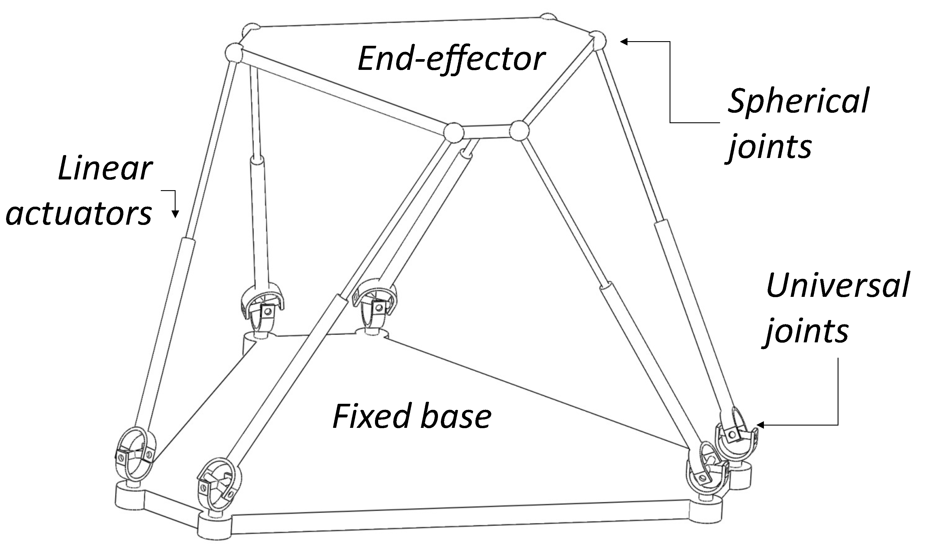
2. Optimization Design Criteria

In this section, we briefly review the kinematics and dynamics of the general Universal Prismatic Spherical (UPS) Gough–Stewart platform to present the necessary concepts for defining the objective functions of the optimization problems.

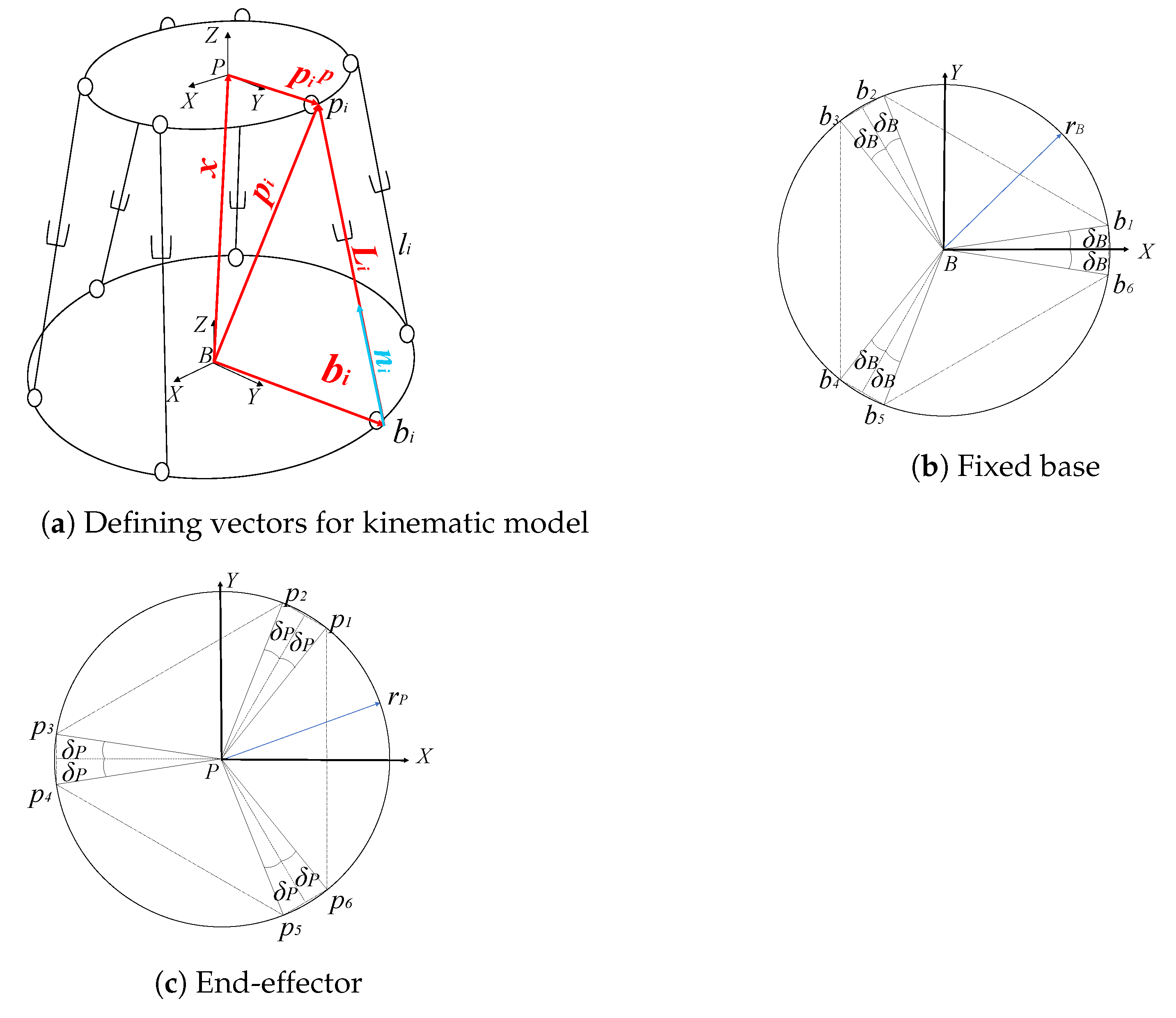
2.1. Kinematics Computation

To define a reachable workspace, we need the computation of the inverse kinematics of the system in order to obtain the lengths effected by each linear actuator in terms of the position and orientation, as shown in Equation (1). The Jacobian expression in Equation (2) is derived from the inverse kinematics. It is used for defining the dexterity index.

Thus, the inverse kinematics can be derived from the schematic of Figure 2a. ${\mathit{L}}_{\mathit{i}}$ represents the vector along the linear positioners and ${\mathit{n}}_{\mathit{i}}$ represents its corresponding unit vector, acting in terms of the position $\mathit{x}$ and orientation in the moving platform $[\psi ,\theta ,\varphi ]$, also called the end-effector. Vectors describing the positions of the spherical and universal joints are included to form closed kinematic chains. Thus, ${\mathit{p}}_{\mathit{i}}$ and ${\mathit{b}}_{\mathit{i}}$ denote the position of both spherical and universal joints, respectively, according to the inertial reference framework B, while ${\mathit{p}}_{\mathit{i}}^{\mathit{P}}$ denotes the spherical joint with P as a reference framework. Moreover, the manipulator is assumed to be symmetric, and the locations of the universal and spherical joints are equally distant with a radius $r_B$ in the base (Figure 2b) and $r_P$ in the moving platform (Figure 2c), with equal aperture angles between pairs ${\delta }_B$ and ${\delta }_P$. Thereby, the expression for the lengths $L_i$ can be written as

$$l_i=|{\mathit{L}}_i|=|\mathit{x}+R_P^B{\mathit{p}}_i^P-{\mathit{b}}_i|,$$

(1)

and, after deriving it, we can obtain the Jacobian expression in the next form:

$$\dot{\mathit{l}}=J_1\left[\begin{array}{c}\dot{\mathit{x}}\\ \omega \end{array}\right]=\left[\begin{array}{cc}{\mathit{n}}_{\mathbf{1}}^{\mathit{T}}& {(\frac{R_p^B}{r_P}{\mathit{p}}_{\mathbf{1}}^{\mathit{P}}\times {\mathit{n}}_{\mathbf{1}})}^T\\ ⋮& ⋮\\ {\mathit{n}}_{\mathbf{6}}^{\mathit{T}}& {(\frac{R_p^B}{r_P}{\mathit{p}}_{\mathbf{6}}^{\mathit{P}}\times {\mathit{n}}_{\mathbf{6}})}^T\end{array}\right]\left[\begin{array}{c}\dot{\mathit{x}}\\ \omega \end{array}\right].$$

(2)

In Equation (1), $R_P^B$ corresponds to the rotation matrix, which is derived in this work by following the $z-y-x$ sequence of axis rotation, while the angles $\psi$, $\theta$, and $\varphi$ denote the rotations made about the z, y, and x axis, most commonly known as yaw, pitch, and roll angles, respectively, and trigonometric functions are written in a short form: s denotes $sine$ and c denotes $cosine$.

$$R_P^B=\left[\begin{array}{ccc}c\psi c\theta ,& -s\psi c\theta +c\psi s\theta s\varphi ,& s\psi s\varphi +c\psi s\theta c\varphi ,\\ s\psi c\theta ,& c\psi c\theta +s\psi s\theta s\varphi ,& -c\psi s\varphi +s\psi s\theta c\varphi ,\\ -s\theta ,& c\theta s\varphi ,& c\theta c\varphi ,\end{array}\right].$$

(3)

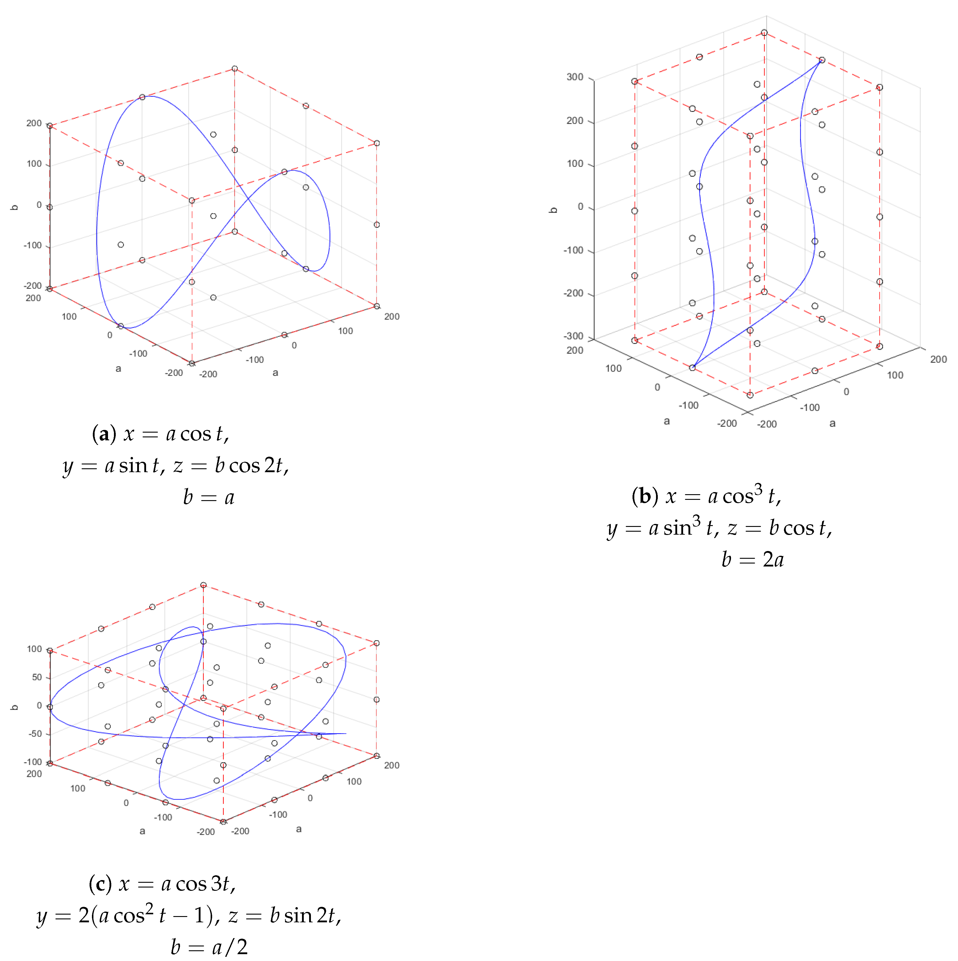
2.2. Regular Workspace Computation Considering Sufficient Dexterity

The optimization algorithms generate candidate length configurations corresponding to the defining sizes of the parallel robot. Each length configuration is called a candidate solution (an individual in the GA context). In order to evaluate them, we must quantify whether they are capable of reaching any point in a set of trajectories with sufficient dexterity. We measure the dexterity of the system with the inverse of the global condition number in Equation (4) using the maximum and minimum singular values of the dimensionally homogeneous Jacobian matrix shown in Equation (2). The dexterity index decreases its value when the robot is close to a singular non-desirable position and increases otherwise. Thus, an acceptable workspace should be restricted to the permitted limits of this value over its complete volume according to the designer’s decision.

$${\kappa }^{-1}=\frac{{\sigma }_{min}\left(J\right)}{{\sigma }_{max}\left(J\right)}.$$

(4)

For this purpose, consider a set of tasks given as target trajectories. They are performed inside a bounding box built by the maximum and minimum coordinates of the target trajectories (see Figure 3) within a limited period. Hence, the platform must be designed to reach, with sufficient dexterity, any point inside such a bounding box.

Here, we introduce the procedure for quantifying the volume of the bounding box reached by a candidate platform. To ensure that the target trajectories lie in allowable dexterity boundaries (in terms of the condition number), the bounding boxes are discretized in points that are spatially distributed along the surfaces and interior, and then, the inverse condition number is evaluated at each of these points. For the case of the cube-shaped trajectory shown in Figure 3a, which is called Trajectory a hereafter,  points are uniformly allocated to ensure their position along the edges, corners, and intermediate positions. This distribution can be seen as the positioning of three equal planes that are parallel to the $xy$ plane and composed of nine points along three different equidistant heights in the z axis, that is to say, a total of 27 points. In a similar way, the trajectory of Figure 3b, called Trajectory b, is discretized by placing the nine-point planes at five equidistant heights of the z axis, resulting in a total of 45 distributed points. For the trajectory of Figure 3c, Trajectory c, it is considered that the bounding box height measures half of the sides’ lengths. Here, sixteen points distributed in planes parallel to $xy$ were placed at three different equidistant heights of z, giving a total of 48 points.

For every candidate solution, namely, the lengths of a Stewart platform, the inverse condition number is evaluated at all of the n discretized points, in which the orientation is maintained constant and parallel to the platform base. If the manipulator is not capable of reaching the total of the bounding box points within the allowable dexterity, and with the stroke limitation of each linear actuator, the candidate solution is not considered suitable.

Mono-Objective Optimization for Dimensional Synthesis

The candidate solutions are generated from a vector of decision variables, which mainly denote the geometrical characteristics of the Stewart platform, $\mathit{d}=[r_B$, $r_P$, ${\delta }_B$, ${\delta }_P$, $l_{max}$, $c_m$]. Here, $l_{max}$ denotes the maximum stroke of the linear actuators, and a last term, $c_m$, is added as a decision variable, indicating the position along the z axis of the center of mass of the bounding box. This way, not only a dimensional synthesis of the robot is made, but also a decision about the best place to locate the trajectory according to this candidate solution.

The objective function in Equation (5) comprises two terms. For the n discretized points, the first term evaluates the competence of the Stewart platform of: (1) reaching the position $x_w$ with the proposed maximum stroke $l_{max}$ and (2) fulfilling the dexterity desired for this point. Each time that a point fulfilling stroke and dexterity conditions is reached, I takes a unit value, and zero otherwise. If all points in the workspace are adequately reached, the sum is equal to n. The second term looks for the minimization of the radius of the base, the radius of the end-effector, and the maximum stroke of the linear actuators. Hence, the optimization parameters of the second term are defined as ${\mathit{d}}_{\mathit{m}}=[r_B/r_B^{max},r_P/r_P^{max},l_{max}/l_{max}^{max}]$. In this vector, the variables to minimize are normalized with respect to their upper boundaries in such a manner that, in the second term of the objective function, the sum does not take a value higher than the unit, and the smaller this value is, the better the dimensional synthesis. Notice that all feasible geometries that reach the whole workspace report an objective value greater than $n-1$, and the best—that with the minimum lengths—is the maximum value.

$$f\left(\mathit{d}\right)=\sum _{w=1}^{n}I\left(x_w\right)-\frac{1}{3}\sum \left|{\mathit{d}}_{\mathit{m}}\right|,$$

(5)

$$\begin{array}{c}\hfill \mathrm{where}I\left(x_w\right)=\left\{\begin{array}{cc}1& \mathrm{if}{\kappa }^{-1}\left(x_w\right)\ge 0.2\mathrm{and}{l}_i<l_{max}\\ 0& \mathrm{otherwise}\end{array}\right\},\end{array}$$

for the $x_w$ positions of the $w=1,\dots n$ discretized points and for the $i=1,\dots 6$ linear actuators. The search limits of the decision variables are given in terms of the bounding boxes’ sizes, as shown in

Table 1. Upper and lower boundaries of the decision variables for the dimensional synthesis.

Trajectory a	Trajectory b	Trajectory c
$0.1a<r_B<3a$	$0.1b<r_B<3b$	$0.1a<r_B<3a$
$0.3a<r_P<3a$	$0.4b<r_P<3b$	$0.4a<r_P<4a$
$5^{\circ }<{\delta }_B<{30}^{\circ }$	$5^{\circ }<{\delta }_B<{30}^{\circ }$	$5^{\circ }<{\delta }_B<{30}^{\circ }$
$7^{\circ }<{\delta }_P<{30}^{\circ }$	$7^{\circ }<{\delta }_P<{30}^{\circ }$	$7^{\circ }<{\delta }_P<{30}^{\circ }$
$0.1a<l_{max}<3a$	$0.1b<l_{max}<3b$	$0.1a<l_{max}<4a$
$b<c_m<5b$	$b<c_m<5b$	$b<c_m<5b$

.

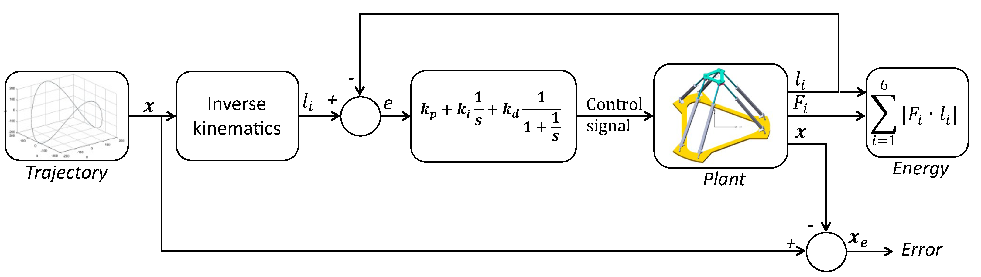
2.3. Computation of the Dynamics

The dynamics of the Stewart platform are solved through the simulation software Simwise 4D [31]. First, the Stewart platform is constructed according to the best geometry obtained in the first stage with the mono-objective optimization using a CAD software; then, the assembly is exported to Simwise 4D for the simulation of the dynamics, with the linear actuators controlled from MATLAB Simulink. This simulation is used to measure the dynamic properties during the tracking of trajectories along with the time steps.

Error and Energy Multi-Objective Optimization

The optimization algorithms look for the minimal accumulated error and energy consumption during the tracking of a trajectory. To this effect, a PID control (see Figure 4) is applied on the linear actuators, which is limited in stroke by the $l_{max}$ resulting from the first stage. Our decision variables are the PID gains for controlling the Stewart platform, which are $\mathit{d}=[k_p,k_i,k_d]$. Similarly to the first stage, decision variables are limited with lower and upper boundaries so that $[0,0,0]\le \mathit{d}\le [2,20,2]$. Notice that the force of the actuators is intrinsically limited by the control gains; hence, they are intrinsically bounded by the search limits. Joint constraints are not considered in this simulation. The PID control law appears in Equation (6).

$$k_p+k_i\frac{1}{s}+k_d\frac{1}{1+\frac{1}{s}}.$$

(6)

The objective function of this second stage is shown in Equation (7). In the first term, it is the integral over the time of the absolute error of the trajectory. The second term is the integral of the absolute multiplication of force times displacement; this term measures a function related to the accumulated energy through the simulation time. Nevertheless, the first lengths have a larger weight than the last because $l_i$ is the total displacement at time t. This objective function helps us to emphasize the energy expended during the initial steps rather than the rest of the trajectory, considering that the initial steps are those with the greatest energy consumption and greatest energy,

$$f\left(\mathit{d}\right)=\left[\begin{array}{c}{\int }_0^t\left|e\right|dt\\ {\int }_0^t\sum \left|F_i·l_i\right|dt\end{array}\right],\mathrm{for}\mathrm{the}i=1,\dots ,6\mathrm{linear}\mathrm{actuators}.$$

(7)

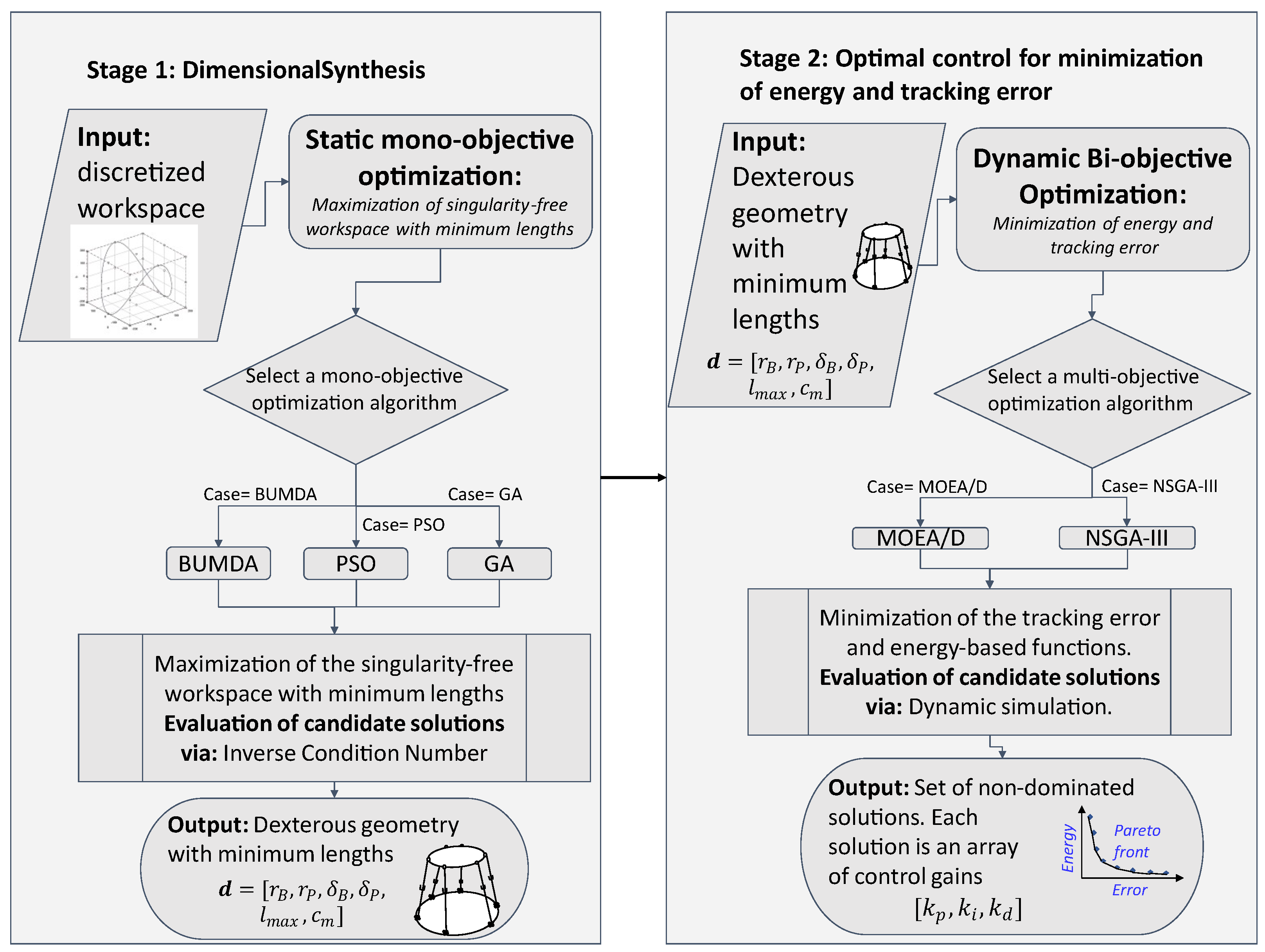
3. Optimization Design Process: Implementation and Results

The integral optimization proposal is defined in two stages as follows:

• Dimensional synthesis of the platform: Using a mono-objective optimization algorithm, we determine the lengths of a platform with minimum dimensions that, with a dexterity measure equal to or greater than 0.2, reaches the points inside a regular workspace.
• Error and energy optimization: Using the lengths of the previous stage and a multi-objective evolutionary algorithm, we approximate the Pareto set, that is, we obtain a set of arrays of gains of the PID controller with the best performance in both objectives.

For Stage 1, we compare three bio-inspired algorithms, and for Stage 2, we compare two multi-objective algorithms from the state of the art. This methodology is briefly explained in Figure 5.

3.1. Mono-Objective Optimization Algorithms

For the workspace optimization, a comparison among three different population-based algorithms was made: the Boltzmann Univariate Marginal Distribution Algorithm (BUMDA) [32], which uses a probabilistic method to sample the optimum values, Particle Swarm Optimization, inspired by flocks of birds or swarming insects [33,34,35], and a Genetic Algorithm based on the research performed by Goldberg [36] and Conn et al. [37,38]. The Particle Swarm Optimization and Genetic Algorithm were taken from the MATLAB routines particleswarm [39] and ga [40].

The PSO used a weight of the neighborhood best and global best equal to 1.49, and the GA used a scattered crossover, that is to say, a binary random array was generated; the positions with 1 were inherited from parent 1; otherwise, they were inherited from parent 2, with a crossover fraction and Gaussian mutation of 0.8.

For the sake of a fair comparison of the mono-objective optimization algorithms, we executed the three algorithms with an equal population size of 50 and 200 maximum iterations, that is, approximately 10,000 maximum function evaluations; the algorithms also stopped if the search suffered stagnation during the last generations. The stagnation of the objective value was measured as follows:

• For the BUMDA, the standard deviation of the objective function values of the population was less than ${10}^{-8}$.
• For the PSO, the relative change in the best objective function value over the last 20 iterations was less than ${10}^{-6}$, or the maximum number of iterations is met. The relative change was computed with the formula $|f_{best}^{20}-f_{best}/max(1,|f_{best}\left|\right)|$, where $f_{best}^k$ is the best function value in the k-th iteration.
• For the GA, the average relative change in the best objective function value over the last 50 generations was less than or equal to ${10}^{-6}$, or the maximum number of iterations is reached. The average relative change was computed as $|f_{best}^1-f_{best}^{50}|/(50·max(1,|f_{best}^{50}\left|\right)$, where $f_{best}^k$ is the best function value in the k-th iteration.

Nevertheless, these settings could favor the BUMDA, which converges faster than the other algorithms, considering that the best results for Trajectory a were [26.561535, 26.560189, 26.502771], for Trajectory b, they were [44.645261,44.714242, 44.620334], and for Trajectory c, they were [47.713794, 45.584584, 39.524893] for the BUMDA, PSO, and GA, respectively. In consequence, we changed the population sizes to the recommended values [39,40] of 60 and 200 for the PSO and GA, respectively. For both cases, the number of iterations was unlimited. Using these last settings, we obtained the results in

Table 2. Mono-objective optimization results: the optimized parameters and best objective function values from 15 independent executions of each algorithm.

Traj.	Alg.	${\mathit{r}}_{\mathit{B}\left(\mathit{mm}\right)}$	${\mathit{r}}_{\mathit{P}\left(\mathit{mm}\right)}$	${\mathit{\delta }}_{\mathit{B}\left(\mathit{rad}\right)}$	${\mathit{\delta }}_{\mathit{P}\left(\mathit{rad}\right)}$	${\mathit{l}}_{\mathit{max}\left(\mathit{mm}\right)}$	${\mathit{c}}_{\mathit{m}\left(\mathit{mm}\right)}$	f	${\mathit{n}}_{\mathit{eval}}$
a	BUMDA	748.45	160.21	0.21	0.23	669.82	1099.29	26.56154	589
	PSO	815.85	120.02	0.12	0.12	647.26	999.99	26.56024	17,100
	GA	876.03	120.03	0.26	0.13	664.66	999.99	26.53869	50,400
b	BUMDA	927.03	151.24	0.19	0.23	837.33	1316.65	44.64526	442
	PSO	592.71	240	0.09	0.12	710.25	1262.62	44.71426	10,080
	GA	691.70	260.54	0.21	0.12	736.93	1296.01	44.68719	20,600
c	BUMDA	495.40	322.40	0.18	0.27	391.22	791.50	47.71379	2843
	PSO	1113.84	160.00	0.11	0.12	578.97	500	47.53664	8100
	GA	988.34	160.04	0.12	0.13	521.48	499.88	45.58347	52,800

. Detailed information about the algorithms’ results can be found by following the “Data Availability” link.

3.2. Multi-Objective Optimization Algorithms

The implementation of two algorithms of different natures [41,42], whose performance has been been recently compared, MOEA/D and NSGA-III [43,44], are executed to find the optimal gains of a PID control given three defined trajectories to track with the end-effector while maintaining a constant orientation. In this second stage, the bi-objective optimization focuses on minimizing the error in the trajectory, as well as the energy consumed. The MOEA/D implementation solves the optimization by decomposing the multi-objective problem into multiple single problems; meanwhile, the NSGA-III proceeds with the Pareto dominance for fitness assignment.

For the sake of completeness, the optimization algorithms were executed with the following parameters: MOEA/D used a weighted crossover as follows: $\alpha ·p1+(1-\alpha )·p2$, where $·$ is a position by position vector multiplication, and $\alpha$ is an array of the same size as the parents, randomly picked from $[-\gamma ,1+\gamma ]$ and $\gamma =0.5$ without mutation, as presented in [41]. NSGA-III used a crossover percentage of 0.5 and mutation percentage of 0.02; it used the same crossover as the MOEA/D, but two children were generated in a single operation from two parents by inverting the positions of the parents. The children mutated a single position using Gaussian mutation with $\sigma =0.1(Va{r}_{max}-Va{r}_{min})$.

3.3. Mono-Objective Optimization Results

Optimization algorithms use stochastic operators; hence, the results may differ one from another. With the intention of obtaining representative results from each algorithm, we executed them 15 times each and performed a statistical analysis to evaluate the performance of the algorithms in solving these problems. In Table 2, we show the best value of the objective function f resulting from this mono-objective stage for each trajectory. These results show the decision variables, that is, the best geometrical configuration of the Stewart platform yielding the best value of the objective function. The last column shows the number of function evaluations required by the algorithm to reach the resulting objective function value. These results are used for the construction of the geometrical models for the tracking of their related trajectories, as shown in Figure 6.

We compared our Stewart platform’s design from Stage 1 with a generic methodology proposed in [45]. In this design method, the author proposed a set of decision variables to define the dimensions of a Stewart platform manipulator; then, he used a simulator to verify that it complied with the desired workspace. If the proposed dimensions do not fit the workspace, then the designer should modify them until a satisfactory solution is found. We applied this methodology to find a configuration for comparing and an objective function value for Trajectory a within the same lower and upper boundaries. The best value found after many iterations in the decision variables was $f\left(\mathit{d}\right)=23.5278$ for the configuration $\mathit{d}=[800,300,0.14,0.40,600,1000]$, while the best values found by the metaheuristics were $26.56152$, $26.56024$, and $26.53869$ by the BUMDA, PSO, and GA, respectively. Despite the many attempts, we could not find a greater value of the objective function with the methodology in [45]. In addition, since f did not meet $f>=n-1$, the desired workspace was not completely fulfilled. In comparison, our methodology found an objective function value greater than $n-1$ and also optimizes it in seconds, while the contrasting method took hours.

Despite the best results obtained with our optimization, we performed statistical analyses among the performances of the algorithms in this stage. This way, we could demonstrate whether one algorithm was better than the others in each trajectory.

Table 3. p-values and acceptance/rejection of the null hypothesis of the Wilcoxon rank sum test and the t-test. × indicates that the left algorithm is better than the right one, while √ indicates that there is not a significant difference between them.

Traj.	Algorithm	Wilcoxon		t-Test
		$\mathit{p}$	$\times /\surd$	$\mathit{p}$	$\times /\surd$
a	BUMDA vs. PSO	$\mathbf{0.000576}$	×	$\mathbf{0.000642}$	×
	BUMDA vs. GA	$0.198456$	√	$0.268204$	√
b	PSO vs. BUMDA	$\mathbf{0.00000}$	×	$\mathbf{0.000003}$	×
	PSO vs. GA	$\mathbf{0.000001}$	×	$\mathbf{0.000003}$	×
c	BUMDA vs. PSO	$0.861813$	√	$0.213323$	√
	BUMDA vs. GA	$\mathbf{0.000007}$	×	$\mathbf{0.000003}$	×

shows a statistical comparison using a non-parametric test, the Wilcoxon rank sum test, and a t-test. These tests evaluated the null hypothesis—that the mean objective values from two algorithms are equal at the 5% significance level. The samples consist in the objective function values f obtained from 15 executions of each algorithm. The rejection of the null hypothesis shows that the two samples compared are significantly different. We compared the algorithms with the best results for each trajectory against the others.

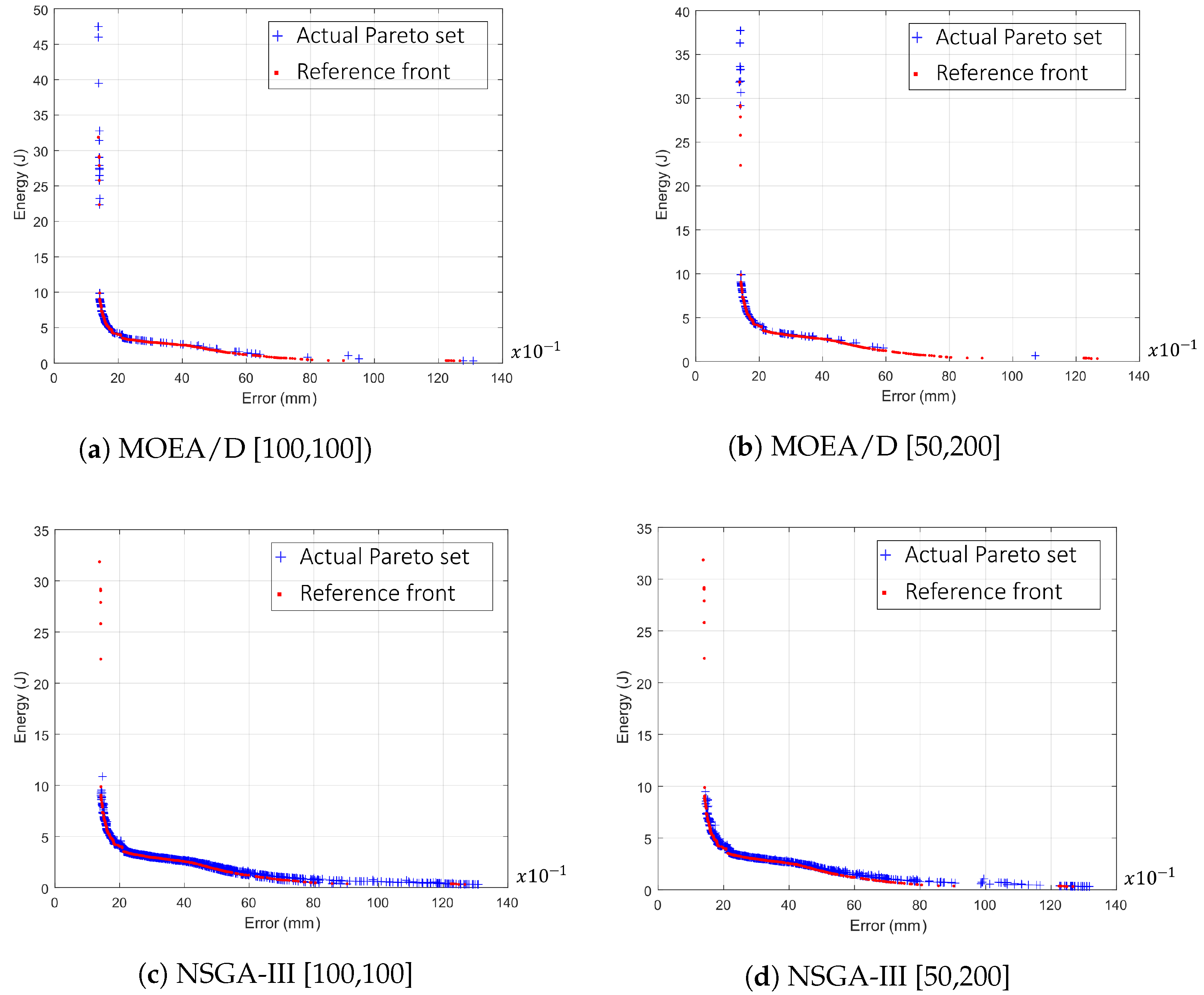
3.4. Multi-Objective Optimization Results

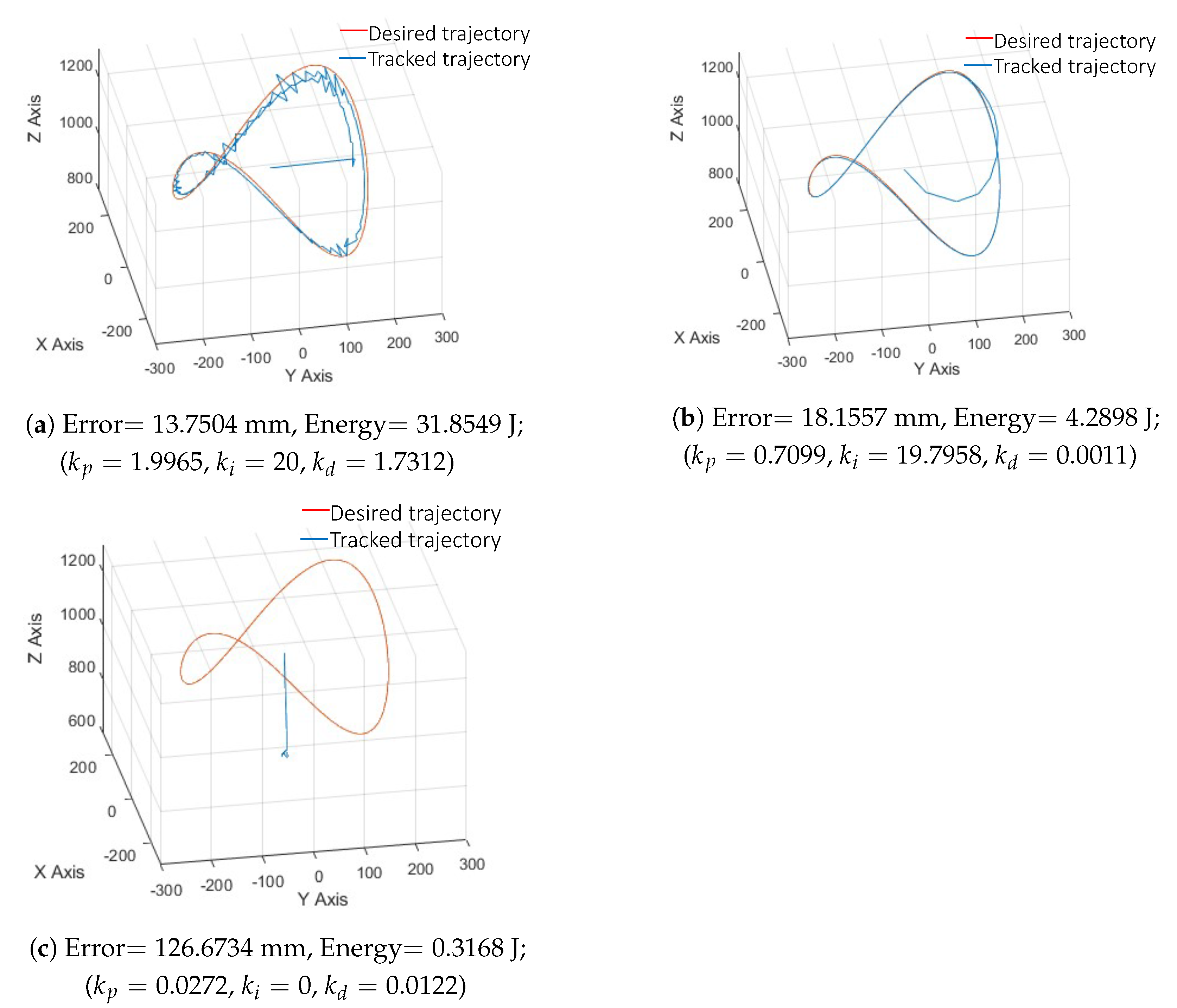
This section shows the results obtained from the multi-objective optimization over Trajectory a. The second stage of this approach yields a set of Pareto solutions that help the designer to decide on the best gains for the PID controllers of the lengths of the actuators, since each individual in the Pareto front is a PID gain combination. The outputs of the optimization algorithms are highly influenced by the population and number of generations used for the executions. We executed the MOEA/D and NSGA-III 15 times with the configurations of $[50,200]$ and $[100,100]$ in population size and generations, respectively (60 total executions). The Pareto sets resulting from all of the executions were combined to yield the reference Pareto front, shown in Figure 7. This Pareto front only considered the non-dominated solutions, shown in red dots, while the dominated (blue crosses) were discarded. Then, each algorithm with the two sets of parameters was compared to the reference Pareto front using performance metrics to find which configuration was the best for the solution of the multi-objective problem. The results from each algorithm separately are depicted in Figure 8. The first performance metric was the Approximated Hypervolume (HV), which, in practical terms, reveals the extension and covering of the Pareto front. The other performance metrics were the Generational Distance (GD) and the Positive Inverse Generational Distance (IGD+); this last metric is a unique weak Pareto-compliant binary metric. These metrics expose how close the current Pareto set is in comparison to the reference one. The lower the value of the GD, the better the proximity to the ideal set, while the IGD+ acts inversely.

Table 4. Averages of performance metrics over the multi-objective results. Best values in bold.

Algorithm [nPop,nGen]	Approx. Hypervolume (Higher Is Better)	Generational Distance (Lower Is Better)	Positive Inverse Generational Distance (Higher Is Better)
MOEA/D [100,100]	$\mathbf{5345.740519}$	$1.823100$	$0.299273$
MOEA/D [50,200]	$3297.389387$	$\mathbf{1.158101}$	$\mathbf{0.348441}$
NSGA-III [100,100]	$1102.987694$	$1.623127$	$0.049558$
NSGA-III [50,200]	$927.873283$	$2.064423$	$0.181521$

shows the metric results obtained from 15 executions of each algorithm configuration. On average, the MOEA/D performed the best, although these average values did not reveal whether the difference between the compared algorithms was statistically significant. In this regard,

Table 5. p-values and acceptance/rejection of the Wilcoxon test and t-test for the multi-objective results of the Positive Inverse Generational Distance (IGD+) for 15 independent executions. Algorithms with statistical differences are in bold. × indicates that the left algorithm is better than the right one, while √ indicates that there is not a significant difference between them.

Algorithm Comparison [nPop,nGen]	Wilcoxon		t-Test
	$p$	$\times /\surd$	$p$	$\times /\surd$
MOEA/D ([100,100] vs. [50,200])	$1.000000$	√	$0.632716$	√
MOEA/D [100,100] vs. NSGA-III [100,100]	$\mathbf{0.000003}$	×	$\mathbf{0.000246}$	×
MOEA/D [100,100] vs. NSGA-III [50,200]	$\mathbf{0.020191}$	×	$0.191011$	√
MOEA/D [50,200] vs. NSGA-III [100,100]	$\mathbf{0.000003}$	×	$\mathbf{0.000004}$	×
MOEA/D [50,200] vs. NSGA-III [50,200]	$\mathbf{0.018054}$	×	$0.231068$	√
NSGA-III ([100,100] vs. [50,200])	$\mathbf{0.000057}$	×	$\mathbf{0.006621}$	×

shows the results of the Wilcoxon test and the t-test to statistically compare the mean of the IGD+ of the 15 independent executions. In the discussion section, we argue that this metric is the best suited for determining the best multi-objective solution from an engineering point of view. As a final result of this stage, we highlighted three results in the Pareto front in Figure 7, corresponding to three different regions of the objective function’s space, that is to say, in the middle and extremes of both objectives. Then, we simulated these optimal results to visually analyze the tracking error; the simulations and their associated PID gains are shown in Figure 9.

4. Discussion

4.1. Mono-Objective Optimization

The results in Table 2 show that the BUMDA delivers the best results for two of the three cases, and the PSO delivers the best result for the other; then, according to Table 3, for the BUMDA for Trajectory a, the tests reject the null hypothesis when comparing the BUMDA to the PSO and accept it when comparing BUMDA with the GA. For the second trajectory, the PSO performs the best, and for the third, the BUMDA is better than the GA, but it is not significantly better than the PSO.

In general, the GA is not the best for any case, and the best algorithm for each trajectory is significantly better than it. Hence, the adequate algorithm selection is between the PSO and the BUMDA. Both algorithms were executed with their default parameters; in this sense, it is possible that the PSO improves its performance if the best execution parameters are used; nevertheless, this requires additional research and computational time for each design problem. On the other hand, the BUMDA requires a single execution parameter, the population size, which is not required to be tuned, according to the recommended settings of 10 times the number of optimization variables [8,32]. Thus, we recommend the use of the BUMDA by default, and to use the PSO if the solution with the BUMDA is not satisfactory or if the trajectory is highly complex, although using the PSO could require one to look for optimal execution parameters.

4.2. Multi-Objective Optimization

The results of the hypothesis tests in Table 5 show that the MOEA/D performed better than the NSGA-III for all cases; nevertheless, there are no statistical differences when using the MOEA/D with different execution parameters. According to the observed results, the largest population size increases the coverage of the Pareto front, while the shortest benefited the convergence. Usually, in the research field of multi-objective optimization, researchers aim to find Pareto front approximations with the maximum extension or coverage of the solution space. Nevertheless, although the results in the Pareto front represent a minimization in one or both objectives, as observed in Figure 7, the extreme solutions that indicate the full extension of the Pareto front are not the most interesting from an engineering point of view, considering that they have the greatest pay-off in the objective functions. That is to say, one extreme of the Pareto front shows a solution that must substantially increase the energy consumption in order to reduce the error by a small quantity, while the second extreme increases the energy for reducing the error with a shorter pay-off than the other. However, even in this case, the solution is not of interest because the energy is too high in contrast with the solutions in the middle, and even though the error is lower than the other solutions, the error signal oscillates due to the large value of the proportional gain, as noticed in Figure 9. Hence, the most useful solutions from an engineering point of view are those with the most balanced pay-off, namely, those in the middle of the Pareto front. For this reason, in the statistical comparison shown in Table 5, we preferred to use the IGD+ metric to emphasize the proximity of the Pareto fronts to the reference instead of using the HV to prioritize the optimality of the solutions rather than the extension of the Pareto front. Once we identified that the middle of the Pareto front was our interest area, comparing the HV was incorrect, since it does not represent the measure of our target. Thus, according to Table 5, we preferred the set of parameters that benefited the convergence, that is, MOEA/D with a population size of 50 and 200 generations.

Table 4 shows the HV of the two algorithms and parameters that were compared. Usually, the performance of multi-objective evolutionary algorithms is measured according to three features: spreading, distribution, and convergence. The first is the extension of the solutions of the approximation of the Pareto front, the second is the representativeness of the solutions—usually, a finite set of equally distributed solutions is desirable to represent a possibly infinite set of optimal solutions—and convergence is measured as the distance to the real Pareto front. The HV measures the first two features; the hypervolume in 2D, such as in this case, is an area measured from the zenith point (the minimum value for each objective) to the points in the Pareto front. Notice that clustered points result in intersecting areas, and the more spread the points are, the larger the covered area is. In this regard, in Table 4, the NSGA-III delivers hypervolumes of approximately one-fifth of the greatest delivered by the MOEA/D, which means that the MOEA/D delivers an approximation to the Pareto front with a larger extension and better-distributed solutions than that delivered by the NSGA-III. In other words, the area generated by the NSGA-III solutions is one-fifth of that delivered by the MOEA/D.

Moreover, the simulation results in Figure 9 confirm that the desired path tracking belongs to the solutions in the middle of the Pareto front, where both error and energy have intermediate values (Figure 9b). In this case, the controller has the greatest gains for the proportional and integrative terms and the lowest for the derivative. For the case in Figure 9a, we see that many oscillations are made around the desired path, and a very abrupt initial step is made because of the high energy expended. This might cause the platform’s elements to experiment with high values of stress, and may also be derived from a failure of the linear actuators, which operate under many limitations, such as the payload and velocities. On the other hand, when the energy is kept at the minimal values, the tracked trajectory is not even close to the expected one (Figure 9c), thus highly increasing the error value. As a final point, notice that even the three presented solutions are not dominated; they are not applicable from an engineering point of view. However, this information is a priori unknown, and the desired solutions can only be selected after the multi-objective optimization.

5. Conclusions

In this work, we introduced a method comprised of two stages for the optimization of the structure and control of a Stewart platform by considering a task of trajectory tracking. The purpose of the two stages is to reduce the computational cost by means of partitioning the three-objective problem into mono-objective and bi-objective sub-problems.

In a first stage, we search for the dimensional synthesis of the structure, reaching a bounding box of the trajectory that fulfills a dexterity index to circumvent singular positions. This process is applied to three different trajectories by means of three optimization algorithms: the BUMDA, PSO, and GA. The BUMDA performs the best most of the time, with a significant difference for Trajectories a and c; meanwhile, for Trajectory b, the best algorithm is the PSO. Hence, we suggest using the BUMDA for dimensional synthesis because of its low computational cost and its use of a single execution parameter. Then, for the second stage, we use the geometry generated by the BUMDA for Trajectory a to model the geometry of the Stewart platform for the second stage.

In the second stage, we look for the best set of gains of a PID controller using the simulation software Simwise 4D for the dynamics of the robot. The MOEA/D and NSGA-III are used for the optimization of the energy and accumulated error. There exists a conflict between the error and energy; in other words, when the error decreases, the energy increases, and vice versa. As a result of this optimization, we obtain a Pareto front approximation and recall that it is unknown until the multi-objective algorithms compute it. Hence, a posteriori, we detect that the most desirable values for the energy and error are those that are most balanced, that is to say, those in the middle of the Pareto front. The associated PID gains for these solutions reveal that the controller acts with a very small derivative gain, with the highest values in the PI terms. In contrast, for the solutions with the smallest values of error, the energy is highly increased, resulting in non-desired oscillations around the trajectory and a very abrupt initial step that might cause the linear positioners to fail. On the contrary, when the energy is the lowest, the error is the highest, making the trajectory highly distant from the desired path.

Since the initial population is selected randomly, the results from algorithms vary in each execution. We executed each algorithm 15 times in the first and second stages to obtain the best results. The samples obtained from the 15 executions were statistically compared through the Wilcoxon rank sum test and t-tests to show which algorithm performed the best for each optimization problem. For the first stage, it was the BUMDA in most of the cases, while in the second stage, the samples for the statistical comparison were made with the IGD+ metric because the interest was in measuring how close the Pareto front approximation was in comparison to the reference front, considering that the best results are located in the middle of the Pareto front, and the solutions in the extremes are not desirable in engineering. Based on this perspective, we observed that the MOEA/D performed better than the NSGA-III in the IGD+ metric, a fact that was further validated by the statistical tests. In this same regard, the population size and iterations were varied for the purpose of obtaining the best execution parameters; they were a population size of 50 and 200 iterations.

For the sake of completeness, three metrics were used for the numerical evaluation of the performance of each algorithm: the Approximate Hypervolume, the Generational Distance, and the Positive Inverse Generational Distance. The MOEA/D performed the best in most cases.

In essence, the main contributions of this work are the proposal of the objective functions and the two-stage method. Furthermore, the implementation of a simulation of the dynamics contributes to decision-makers in selecting practically feasible solutions from a set of optimal solutions. Finally, we contributed with the application of metrics and statistical tests to support the evaluation of the optimization algorithms’ performance and to provide directions for the adequate metaheuristics for this problem.

References

1. Sun, T.; Lian, B. Stiffness and mass optimization of parallel kinematic machine. Mech. Mach. Theory 2018, 120, 73–88. [Google Scholar] [CrossRef]
2. Pedrammehr, S.; Mahboubkhah, M.; Khani, N. A study on vibration of Stewart platform-based machine tool table. Int. J. Adv. Manufac. Technol. 2013, 65, 991–1007. [Google Scholar] [CrossRef]
3. Pugazhenthi, S.; Nagarajan, T.; Singaperumal, M. Optimal trajectory planning for a hexapod machine tool during contour machining. Proc. Inst. Mech. Eng. Part C J. Mech. Eng. Sci. 2002, 216, 1247–1256. [Google Scholar] [CrossRef]
4. Geng, Z.; Haynes, L.S. Six-degree-of-freedom active vibration isolation using a stewart platform mechanism. J. Robot. Syst. 1993, 10, 725–744. [Google Scholar] [CrossRef]
5. Kazezkhan, G.; Xiang, B.; Wang, N.; Yusup, A. Dynamic modeling of the Stewart platform for the NanShan Radio Telescope. Adv. Mech. Eng. 2020, 12, 1–10. [Google Scholar] [CrossRef]
6. Keshtkar, S.; Hernandez, E.; Oropeza, A.; Poznyak, A. Orientation of radio-telescope secondary mirror via adaptive sliding mode control. Neurocomputing 2017, 233, 43–51. [Google Scholar] [CrossRef]
7. Velasco, J.; Calvo, I.; Barambones, O.; Venegas, P.; Napole, C. Experimental Validation of a Sliding Mode Control for a Stewart Platform Used in Aerospace Inspection Applications. Mathematics 2020, 8, 2051. [Google Scholar] [CrossRef]
8. Botello-Aceves, S.; Valdez, S.I.; Becerra, H.M.; Hernandez, E. Evaluating concurrent design approaches for a Delta parallel manipulator. Robotica 2018, 36, 697–714. [Google Scholar] [CrossRef]
9. Valdez, S.I.; Botello-Aceves, S.; Becerra, H.M.; Hernández, E.E. Comparison Between a Concurrent and a Sequential Optimization Methodology for Serial Manipulators Using Metaheuristics. IEEE Trans. Ind. Inform. 2018, 14, 3155–3165. [Google Scholar] [CrossRef]
10. Panda, S.; Mishra, D.; Biswal, B. Revolute manipulator workspace optimization: A comparative study. Appl. Soft Comput. 2013, 13, 899–910. [Google Scholar] [CrossRef]
11. Badescu, M.; Mavroidis, C. Workspace Optimization of 3-Legged UPU and UPS Parallel Platforms with Joint Constraints. J. Mech. Des. 2004, 126, 291–300. [Google Scholar] [CrossRef]
12. Lou, Y.; Liu, G.; Chen, N.; Li, Z. Optimal design of parallel manipulators for maximum effective regular workspace. In Proceedings of the 2005 IEEE/RSJ International Conference on Intelligent Robots and Systems, Edmonton, AB, Canada, 2–6 August 2005; pp. 795–800. [Google Scholar] [CrossRef]
13. Dereli, S.; Köker, R. A meta-heuristic proposal for inverse kinematics solution of 7-DOF serial robotic manipulator: Quantum behaved particle swarm algorithm. Artif. Intell. Rev. 2016, 53, 949–964. [Google Scholar] [CrossRef]
14. Falconi, R.; Grandi, R.; Melchiorri, C. Inverse Kinematics of Serial Manipulators in Cluttered Environments using a new Paradigm of Particle Swarm Optimization. IFAC Proc. Vol. 2014, 47, 8475–8480. [Google Scholar] [CrossRef] [Green Version]
15. Al-Dois, H.; Jha, A.K.; Mishra, R.B. Task-based design optimization of serial robot manipulators. Eng. Optim. 2013, 45, 647–658. [Google Scholar] [CrossRef]
16. Kuçuk, S. Optimal trajectory generation algorithm for serial and parallel manipulators. Robot. Comput. Integrat. Manufac. 2017, 48, 219–232. [Google Scholar] [CrossRef]
17. Ravichandran, R.; Heppler, G.; Wang, D. Task-based optimal manipulator/controller design using evolutionary algorithms. Proc. Dynam. Control Syst. Struc. Space 2004, 1–10. [Google Scholar]
18. Boudreau, R.; Gosselin, C.M. The Synthesis of Planar Parallel Manipulators with a Genetic Algorithm. J. Mech. Des. 1999, 121, 533–537. [Google Scholar] [CrossRef]
19. Patel, S.; Sobh, T. Task based synthesis of serial manipulators. J. Adv. Res. 2015, 6, 479–492. [Google Scholar] [CrossRef] [PubMed] [Green Version]
20. Lou, Y.; Zhang, Y.; Huang, R.; Chen, X.; Li, Z. Optimization Algorithms for Kinematically Optimal Design of Parallel Manipulators. IEEE Trans. Autom. Sci. Eng. 2014, 11, 574–584. [Google Scholar] [CrossRef]
21. Soltanpour, M.R.; Khooban, M.H. A particle swarm optimization approach for fuzzy sliding mode control for tracking the robot manipulator. Nonlinear Dyn. 2013, 74, 467–478. [Google Scholar] [CrossRef]
22. Zhang, X.; Nelson, C.A. Multiple-Criteria Kinematic Optimization for the Design of Spherical Serial Mechanisms Using Genetic Algorithms. J. Mech. Des. 2011, 133, 011005. [Google Scholar] [CrossRef]
23. Miller, K. Optimal Design and Modeling of Spatial Parallel Manipulators. Int. J. Robot. Res. 2004, 23, 127–140. [Google Scholar] [CrossRef]
24. Yang, C.; Li, Q.; Chen, Q. Multi-objective optimization of parallel manipulators using a game algorithm. Appl. Math. Modell. 2019, 74, 217–243. [Google Scholar] [CrossRef]
25. Hultmann Ayala, H.V.; dos Santos Coelho, L. Tuning of PID controller based on a multiobjective genetic algorithm applied to a robotic manipulator. Expert Syst. Appl. 2012, 39, 8968–8974. [Google Scholar] [CrossRef]
26. Zhang, D.; Gao, Z. Forward kinematics, performance analysis, and multi-objective optimization of a bio-inspired parallel manipulator. Robot. Comput. Integrat. Manufac. 2012, 28, 484–492. [Google Scholar] [CrossRef]
27. Cirillo, A.; Cirillo, P.; De Maria, G.; Marino, A.; Natale, C.; Pirozzi, S. Optimal custom design of both symmetric and unsymmetrical hexapod robots for aeronautics applications. Robot. Comput. Integrat. Manufac. 2017, 44, 1–16. [Google Scholar] [CrossRef]
28. Joumah, A.A.; Albitar, C. Design Optimization of 6-RUS Parallel Manipulator Using Hybrid Algorithm. Mod. Educ. Comput. Sci. Press 2018, 10, 83–95. [Google Scholar] [CrossRef] [Green Version]
29. Nabavi, S.N.; Shariatee, M.; Enferadi, J.; Akbarzadeh, A. Parametric design and multi-objective optimization of a general 6-PUS parallel manipulator. Mech. Mach. Theory 2020, 152, 103913. [Google Scholar] [CrossRef]
30. Lara-Molina, F.A.; Rosário, J.M.; Dumur, D. Multi-Objective Design of Parallel Manipulator Using Global Indices. Benthnam Open 2010, 4, 37–47. [Google Scholar] [CrossRef] [Green Version]
31. SimWise 4D. 2020. Available online: https://www.design-simulation.com/SimWise4d/ (accessed on 1 March 2021).
32. Valdez, S.I.; Hernández, A.; Botello, S. A Boltzmann based estimation of distribution algorithm. Inform. Sci. 2013, 236, 126–137. [Google Scholar] [CrossRef]
33. Kennedy, J.; Eberhart, R. Particle swarm optimization. In Proceedings of the ICNN’95—International Conference on Neural Networks, Perth, WA, Australia, 27 November–1 December 1995; Volume 4, pp. 1942–1948. [Google Scholar] [CrossRef]
34. Mezura-Montes, E.; Coello Coello, C.A. Constraint-handling in nature-inspired numerical optimization: Past, present and future. Swarm Evolution. Comput. 2011, 173–194. [Google Scholar] [CrossRef]
35. Pedersen, M.E. Good Parameters for Particle Swarm Optimization; Hvass Laboratories: Luxembourg, 2010. [Google Scholar]
36. Goldberg, D.E. Genetic Algorithms in Search, Optimization and Machine Learning, 1st ed.; Addison-Wesley Longman Publishing Co. Inc.: Boston, MA, USA, 1989. [Google Scholar]
37. Conn, A.R.; Gould, N.I.M.; Toint, P.L. A Globally Convergent Augmented Lagrangian Algorithm for Optimization with General Constraints and Simple Bounds. SIAM J. Num. Anal. 1991, 28, 545–572. [Google Scholar] [CrossRef] [Green Version]
38. Conn, A.R.; Gould, N.I.M.; Toint, P.L. A Globally Convergent Augmented Lagrangian Barrier Algorithm for Optimization with General Inequality Constraints and Simple Bounds. Math. Comput. 1997, 66, 261–288. [Google Scholar] [CrossRef]
39. MATLAB, Help Particleswarm, Mathworks. 2020. Available online: https://www.mathworks.com/help/gads/particleswarm.html (accessed on 1 March 2021).
40. MATLAB, Help ga, Mathworks. 2020. Available online: https://www.mathworks.com/help/gads/ga.html (accessed on 1 March 2021).
41. Yarpiz. Multi-Objective Evolutionary Algorithm based on Decomposition (MOEA/D). 2016. Available online: https://yarpiz.com/456/ypea126-nsga3 (accessed on 1 March 2021).
42. Yarpiz. Implementation of Non-Dominated Sorting Genetic Algorithm III in MATLAB. 2015. Available online: https://yarpiz.com/95/ypea124-moead (accessed on 1 March 2021).
43. Deb, K.; Jain, H. An Evolutionary Many-Objective Optimization Algorithm Using Reference-Point-Based Nondominated Sorting Approach, Part I: Solving Problems With Box Constraints. IEEE Trans. Evolution. Comput. 2014, 18, 577–601. [Google Scholar] [CrossRef]
44. Li, H.; Deb, K.; Zhang, Q.; Suganthan, P.; Chen, L. Comparison between MOEA/D and NSGA-III on a set of novel many and multi-objective benchmark problems with challenging difficulties. Swarm Evolution. Comput. 2019, 46, 104–117. [Google Scholar] [CrossRef]
45. Gong, Y. Design Analysis of a Stewart Platform for Vehicle Emulator Systems. Master’s Thesis, Department of Mechanical Engineering, Massachusetts Institute of Technology, Cambridge, MA, USA, 1992. [Google Scholar]
Figure 1. General scheme of the 6–6 degree-of-freedom (DOF) Stewart platform mechanism.
Mathematics 09 00543 g001
Figure 2. General Universal-Prismatic-Spherical (UPS) Gough-Stewart structure. Stage 1 looks for the optimal r B , r P , δ B , δ P , and maximum stroke l m a x to cover a dexterous workspace. Stage 2 uses the resulting geometry to provide an optimal dynamic control.
Mathematics 09 00543 g002
Figure 3. Target trajectories, named hereafter (ac), labelled correspondingly, within prismatic bounding boxes, and points of the discretized workspace.
Mathematics 09 00543 g003
Figure 4. Proportional Integral Derivative (PID) control scheme of the lengths. It is used for the error and energy optimization.
Mathematics 09 00543 g004
Figure 5. Flowchart of the general optimization process. Stage 1, on the left, finds the geometrical configuration, and Stage 2, on the right, finds the optimal control parameters. Notice that both stages are connected.
Mathematics 09 00543 g005
Figure 6. Results for dimensional synthesis based on target trajectories.
Mathematics 09 00543 g006
Figure 7. The non-dominated Pareto front versus the dominated error–energy values of both the MOEA/D and NSGA-III executions; labeled points are the configurations in Figure 9.
Mathematics 09 00543 g007
Figure 8. Pareto front from individual configurations of MOEA/D and NSGA-III from 15 independent executions. (a) MOEA/D with population size of 100 and 100 generations, (b) MOEA/D with population size of 50 and 200 generations, (c) NAGS-III with population size of 100 and 100 generations, and (d) NSGA-III with population size of 50 and 200 generations.
Mathematics 09 00543 g008
Figure 9. Three different simulations from the extremes and middle of the obtained Pareto front of Figure 7 and associated PID gains. (a) Low error but high energy consumption; (b) an error–energy balance; (c) denotes low energy but high error.
Mathematics 09 00543 g009