Abstract
In this paper, we have obtained three optimal order Newton’s like methods of order four, eight, and sixteen for solving nonlinear algebraic equations. The convergence analysis of all the optimal order methods is discussed separately. We have discussed the corresponding conjugacy maps for quadratic polynomials and also obtained the extraneous fixed points. We have considered several test functions to examine the convergence order and to explain the dynamics of our proposed methods. Theoretical results, numerical results, and fractal patterns are in support of the efficiency of the optimal order methods.
1. Introduction
Finding the solutions of nonlinear equations or transcendental equations is the core problem in applied science, technology, and engineering because often the main problem ultimately reduces to it of the form
Generally, we are unable to find its exact practical solutions by known algebraic methods. Hence, we are bound to use numerical methods to obtain its approximate solutions. We can determine the solutions of (1) as a fixed point of some iteration function g by means of the one-point iteration method. Let be a simple zero, i.e., of a function for an open interval I and . Here, is a continuously differentiable real valued function and symbols have their usual meaning. Consider the fixed point iterative problem
where is the initial value. The most important known and the most basic used example of these types of methods is the classical Newton’s method given by
However, its limitation is that it is only of order two under some conditions. In the literature, several authors have made modifications and refinements of Newton’s method to speed it up or to find a better method by using different techniques i.e., adding functions terms, derivatives terms, and/or by variations in the points of iterations [1,2]. Singh [3] developed a six-order variant of Newton’s method for simple roots in 2009. In the same year, Maheshwari [4] gave an optimal fourth-order iterative method for solving nonlinear equations defined by
where
Recently, we could see a lot of papers in literature with topics related to optimal order methods and dynamics. For example, Kung and Traub [5] introduced an optimal order of one-point and multipoint iteration in 1974. Cordero et al. [6] described a three-step iterative methods with optimal eighth-order convergence in 2011, while Sharma et al. [7] gave an optimal eighth order convergent iteration scheme based on Lagrange interpolation in 2017. Ashish et al. [8] described the Julia sets and Mandelbrot sets in Noor orbit in 2014. Neta et al. described the basin attractors for various methods in 2011 [9]. A comparison between iterative methods by using the basins of attraction was developed by Ardelean [10]. It motivates us to work on the optimal order methods with their basins of attraction. We have obtained three optimal order (four, eight, and sixteen) iterative methods using a new different technique. This technique is more simple to previous one developed by Tao et al. [2]. We have developed the optimal order methods by repeated applications of Newton’s method and thereafter approximated the derivative term in Newton’s method by a suitable polynomial to reduce the functions evaluations and obtained the optimal order methods. The efficiency of the optimal order methods is tested using several numerical examples. We obtained the extraneous fixed points and discussed the corresponding conjugacy maps for quadratic polynomials. Lastly, we have discussed the dynamics of our methods and found that the basin of attraction for different order methods is also in support of numerical results.
2. Preliminary
Definitions
Definition 1
(see [11,12]). If be k approximations to the root, then an iterative method defined as
is called multi-point iteration method and the function g is called multi-point iteration function. For , we get the one point iteration method
Definition 2
(see [11,12]). A sequence of iterates is said to converge to a limit with order , if
where , is known as asymptotic error constant. In case of , the method is said to converge linearlly.
If we denote , then an error equation of pth order method can be written as .
Definition 3
(see [11,12]). For a pth order iterative method, the efficiency index may be defined as , where m is the total number of functions and derivatives’ evaluations at each iteration. Therefore, the Newton’s method has efficiency index 1.414 and our proposed optimal sixteenth order method has efficiency index 1.741.
Definition 4
(see [11,13]). According to Kung–Traub conjecture formula, an iterative Newton’s like method is called an optimal order method if its order is where n is the number of functions’ evaluation. For example, the second-order Newton’s method requiring two functions evaluation is an optimal order method. Similarly, the fourth-order Maheshwari method is an optimal method and our sixteenth-order proposed method requiring five functions evaluation is also an optimal order method according to Kung–Traub conjecture formula.
Next, we will define the following definitions but in the extended complex plane.
Definition 5
(see [9,14]). Let I be a subset of C. Let us consider the map g : I → C be a rational map on the Riemann sphere, then a point is said to be a fixed point of g, if
Again, for any point , the Orbit of the point z can be defined as the set
Definition 6
(see [9,14]). A periodic point is said to be of period k, if there exists a smallest positive integer k i.e., . If is periodic point of period k, then clearly it is a fixed point for .
Definition 7
(see [9,14]). Let be a root of function f, then the basin of attraction of the root is defined as the set of all initial approximations such that any numerical iterative method with converges to . It can be written as
where is any fixed point iterative method.
Remark 1.
For example, in the case of Newton’s method,
We can write the basin of attraction of the zero for the Newton’s method as follows:
Definition 8
(see [14]). Let I be a subset of C. Let us consider the map g : I → C be a rational map on the Riemann sphere, then a fixed point of map g is a said to be a
- attracting if and only if
- super-attracting if and only if
- repelling if and only if
From the above definition, it is clear that all the fixed points of the Newton’s method are super attracting fixed points, as if ; then, for Newton’s method, we have
Hence, is super attracting fixed points for the Newton’s method.
Definition 9
(see [9,14]). The Julia set for a nonlinear map g(z) is denoted as , and is defined as a set consisting of the closure of its repelling periodic points. The complement of Julia set is called the Fatou set .
Remark 2.
(i) Sometimes, the Julia set of a nonlinear map may also be defined as the common boundary shared by basins of the roots and the Fatou set may also be defined as the set which contains the basin of attraction.
(ii) Fractals are very complicated phenomenon may be defined as a self-similar surprising geometric object which repeats at every small scale. Benoit Mandelbrot is known as the father of fractal geometry. He explains geometric fractals as “a rough or fragmented geometric shape that can be divided into parts, every one of which is a reduced-size duplicate of the whole” [15]. There is a lot of variety of fractals found in nature in the form of many usual objects such as mountains, coastlines, tree ferns, peacock’s feather, and clouds.
3. Description of Method
We start with optimal order quadratically convergent classical Newton’s method given by
3.1. An Optimal 4th Order Method
Let us again apply Newton’s method, and we have
This is a fourth-order method having four functions’ evaluations and hence is not an optimum method. To reduce the function evaluations and preserve the order of convergence to be optimum, we estimate by the following polynomial:
satisfying the following conditions:
We use the following difference notation:
Applying the above conditions on Equation , we have
Since , we can write
Hence, a new optimal fourth-order method will be
We already know that Newton’s method with a two functions evaluation has i.e., second-order convergence. Hence, Newton’s method is optimal according to Kung–Traub conjecture. Now, we will prove that the proposed method represented by (9) is optimal fourth-order according to Kung–Traub conjecture as follows:
Theorem 1.
Let I be an open interval in ℜ and be a function such that
(i) is a simple zero of a function f,
(ii) at the zero and
(iii) f is sufficiently differential in the open set I at some neighborhood S of the zero .
Then, the proposed Newton’s like Method defined by has fourth-order convergence to the zero of f locally.
Proof.
Let be a simple zero of f. Let and . Then, applying the Taylor’s expansion of about and using , we have
We get from the above equations
Using Newton’s method, we have
Hence, from Equation (9), we have
Now, using the fact that , we get
The above Equation (14) shows that multi points (two-points) Newton’s like method (9) with three functions evaluation has th order convergence to the root of f locally, provided f is 4th order differentiable in I. Hence, the method is optimal according to Kung–Traub conjecture. □
3.2. An Optimal 8th Order Method
Now, we will proceed to obtain an optimal eighth-order method:
Above is the eighth-order method, which requires five functions’ evaluations, hence it is not an optimal method. To make it optimal, we reduce the function evaluations and preserve the order of convergence. We estimate by the following polynomial:
satisfying the following conditions:
and, using we have
Applying the finite difference formula and solving the above nonlinear equations, we get the value of , and as follows:
Hence, we have
We can write
Hence, the new optimal eighth-order method will be
Next, we will theoretically show that the above proposed method (15) is an optimal eighth-order method.
Theorem 2.
Let I be an open interval in ℜ and be a function such that
(i) is a simple zero of a function f,
(ii) at the zero and
(iii) f is sufficiently differential in the open set I in some neighborhood S of the zero .
Then, the proposed Newton’s like Method defined by has eighth-order convergence to the zero of f locally.
Proof.
Let be a simple zero of a function f i.e., . Let and . Now, applying the Taylor’s expansion of about and using , we get
Now, from the above, we get
Using , we obtain
Substituting the values in (15), we have
Now, using , we get
This shows that Newton’s like method (15) with four functions evaluation has = 8th order convergence to the root of f locally, if f is differentiable up to eighth-order in open interval I. Hence, the proposed method (15) is 8th order optimal method according to Kung–Traub conjecture. □
3.3. An Optimal 16th Order Method
Next, we will obtain an optimal 16th order method
Above is the sixteenth-order method, which requires six functions’ evaluations; hence, it is not an optimal order method. We make it optimal by reducing the function by the following polynomial:
satisfying the following conditions:
Applying the above conditions and using and , we have
We find the values of . These are very large expressions. The value of will be as follows:
We can write
Hence, the new optimal sixteen-order method will be
Now, we will prove the convergence analysis theorem for the proposed method (20) to show that it is an optimal 16th order method.
Theorem 3.
Let I be an open interval in ℜ and be a function such that
(i) is a simple zero of a function f,
(ii) at the zero and
(iii) f is sufficiently differential in the open set I in some neighborhood S of the zero .
Then, the proposed Newton’s like Method defined by Equation has sixteenth-order convergent to the zero of f locally.
Proof.
Let be a simple zero of a function f i.e., . Let and . Now, applying the Taylor’s expansion of about and using , we get
Now, we get from above,
Using , we obtain
From Equation (20), we have
Using the above equation, we have
Equation (25) confirms that the proposed Newton’s like method (20) with five function evaluation has = 16th order convergence to the root of f locally, if f is differentiable up to sixteenth-order in open interval I in some neighborhood S of the zero . Hence, the method is 16th order optimal according to Kung–Traub conjecture. □
4. Numerical Results
In this section, we display the numerical results of some test problems to examine the efficiency of proposed new optimal order methods. We have compared the proposed optimal order methods with Maheshwari 4th order method [4], Tao et al. 8th order method [2], and Sharma et al. 8th order method [16]. The following test functions have been used for this purpose:
In Table 1, N, F, D, and PM denote the number of iterations, failure of the method, divergence of the method, and proposed method, respectively. Numerical computations reported here have been performed in MATLAB using the stopping criterion as .

Table 1.
Comparison of the different methods with the present methods.
In numerical observations, we have taken the same two points −10 and 50 for all the test functions. From Table 1, we can observe that Newton’s method fails for the function , , and at both the points −10 and 50, but it should be noted that it fails only due to the tighter stopping criteria. Similarly, the fourth-order Maheshwari method and fourth-order proposed method are diverging for the functions at both points −10 and 50, while the proposed 16th order method is best among all the methods by taking the least number of iterations.
In Table 2, we have listed the efficiency index of different methods. We can observe from Table 2 that the efficiency index of 16th order proposed optimal method is 1.741, which is highest among all the methods.
Table 2.
Comparison of the efficiency index of different methods.
Planck’s Radiation Law Problem
We have solved the Planck’s radiation law problem taken from the [17], which is also solved by Tao et al. in his paper [2]. Planck’s radiation law is given by the following formula:
which relates the energy density within an isothermal blackbody. Here,
is the wavelength of the radiation,
T is the absolute temperature of the blackbody,
k is the Boltzmann’s constant,
h is the Planck’s constant,
c is the velocity of light.
Now, we have to find the value of wavelength in such a way that energy density is maximum. From (26), we get
We claim that F will be maximum when the second term in the bracket will be equal to zero
Letting x= ch/kT, then we have
Define
Now, we have to find the solution or root of the Clearly, x = 0 is one root, but it is useless; Equation (27) reveals that another root might be near at the point x = 5.0. Hence, stating with the initial approximation , an approximate solution of (27) is given by . Therefore, the wavelength of radiation () corresponding to the maximum energy density will be approximated as
We can observe from Table 3 that the proposed 16th order method converges to the root in only one iteration with minimum error, hence performing better than the other methods.
Table 3.
Comparison of different methods for the Planck Radiation problem at .
5. Corresponding Conjugacy Maps for Quadratic Polynomials
In this section, we will discuss the rational map arising from various methods applied to a generic polynomial with simple zeros.
Theorem 4
(Newton method). For a rational map arising from Newton method (3) applied to , , is conjugate via the Mobius transformation given by to
where
Theorem 5
(Maheshwari method [4]). For a rational map arising from Maheshwari method applied to , , is conjugate via the Mobius transformation given by to
where
Theorem 6
(Sharma et al. [16]). For a rational map arising from Sharma et al. method applied to , , is conjugate via the Mobius transformation given by to
where
Theorem 7
(Proposed 4th order method). For a rational map arising from proposed 4th order method (9) applied to , , is conjugate via the Mobius transformation given by to
where
Theorem 8
(Newton like method). For a rational map arising from proposed Newton like method (15) and (20) and method of Tao et al. [2] to , , is conjugate via the Mobius transformation given by to
where is either unity or a rational function and p is the order of the proposed Newton like method (15) and (20) and method of Tao et al. [2].
6. Extraneous Fixed Points
The proposed optimal order Newton like iterative methods discussed in Section (3) along with 4th order Maheshwari method [4], 8th order method of Tao et al. [2] and 8th order method of Sharma et al. [16] can be written in the fixed-point iteration form as
Clearly, the root of is a fixed point of the method. However, the points at which are also fixed points of the method as, with , the second term on the right side of (28) vanishes. These points are called extraneous fixed points (see [18]). We have already discussed the different type of fixed point in the definition section. In this section, we will discuss the extraneous fixed points of some Newton like method for the polynomial .
Theorem 9.
There are no extraneous fixed points for the Newton method:
Proof.
For the Newton method, we have Hence, it has no extraneous fixed point. □
Theorem 10.
There are 18 extraneous fixed points for the Maheshwari method given by Equation (4).
Proof.
For Maheshwari method (4), given by the following equation:
.
In this equation, the numerator is of degree 18 and, hence, the Maheshwari method has 18 extraneous fixed points:
These fixed points are repelling (the derivative at these points has its magnitude ). □
Theorem 11.
There are 42 extraneous fixed points for the method of Sharma et al. [16].
Proof.
For the method of Sharma et al. (6), we have given by the following equation:
In this equation, the numerator is of degree 42 and, hence, it has 42 extraneous fixed points. These fixed points are repelling (the derivative at these points has its magnitude ). □
Theorem 12.
There are nine extraneous fixed points for the proposed 4th order method (9).
Proof.
For the proposed 4th order method, we have given by the following equation: In this equation, the numerator is of degree 9 and, hence, it has nine extraneous fixed points:
z = −0.818252548214172417440501524875 − 0.193036788681890093692392888421i,
z = −0.818252548214172417440501524875 + 0.193036788681890093692392888421i,
z = −0.512818196864335208967348203500,
z = 0.241951511243600984239351795067 − 0.805145887805769566603684565559 i,
z = 0.241951511243600984239351795067 +0.805145887805769566603684565559 i,
z = 0.2564090984321676044836741017502 − 0.4441135860074436480571086381193 i,
z = 0.2564090984321676044836741017502 + 0.4441135860074436480571086381193 i,
z = 0.576301036970571433201149729808 − 0.612109099123879472911291677137 i,
z = 0.576301036970571433201149729808 + 0.612109099123879472911291677137 i.
These fixed points are repelling (the derivative at these points has its magnitude ). □
Theorem 13.
There are 39 extraneous fixed points for the proposed 8th order method (15).
Proof.
For the proposed 8th order method, we have given by the following equation:
.
In this equation, the numerator is of degree 39, and hence it has 39 extraneous fixed points. □
Remark 3.
Similarly, we may calculate the extraneous fixed points for other Newton-like methods. These fixed points are repelling (the derivative at these points has its magnitude ). These fixed points can be seen in the fractal patterns graph of the basins of attraction for (see Figure 5).
7. Dynamics of the Methods
In this section, we have considered some test examples to examine the basin of attraction of various methods. The problem of determining the basins of attraction for complex functions is also known as Cayley’s problem. Basins of attraction of the zeros of function f(z) sharing a common boundary called the Julia set of f(z) [19]. In this case, any point on the boundary of one set also lies on the boundary of the other sets. Basins of attraction with a specific property in which any point on the one-set boundary also lies on the other-sets boundary are known as the Wada property, given by Japanese mathematician Yoneyama in 1917 [20]. Due to the Wada property, any neighborhood of a point on the boundary of the basin of attraction will contain other different points due to which the iteration process will flow to each root. In particular, trajectories corresponding to close starting points on the boundary will have divergent orbits. Hence, the boundary points of Julia set describe the instability for any given approximation.
Therefore, we may conclude from above that the study of dynamics of the test functions with the help of an iterative method allows us to study the important information about convergence, divergence, and stability of the methods. The basic definitions and dynamical concepts related to fractal and basins can be found in [14,21].
7.1. For Inner Functions .
We apply our numerical iterative methods in a square of points with a tolerance- and a maximum of 15 iterations. Under the above conditions, starting with every point in the square, if the sequence generated by the iterative methods converge to a zero of the function, then will be in the basin of attraction of this zero, and we mark this point with a fixed color. We have described the basins of attraction for 2nd order Newton’s method, 4th order Maheshwari method, 4th order proposed method, 8th order Tao et al. method [2], 8th order Sharma et al. method [16], 8th order proposed method, and the 16th order proposed method for finding complex roots of some test functions, which we have considered earlier, e.g.,
The basins of attraction of the zeros for considered test functions by different methods have been shown in Figure 1, Figure 2, Figure 3 and Figure 4, respectively. We conclude from the figures as follows:
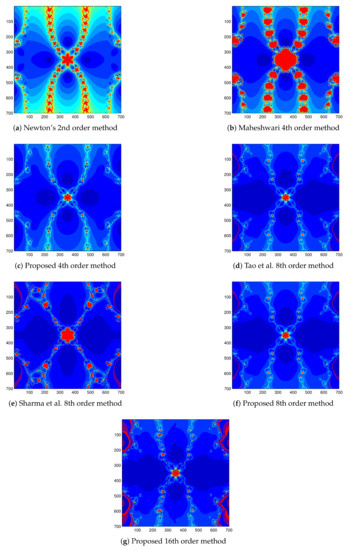
Figure 1.
Basin of attraction for , by different methods.
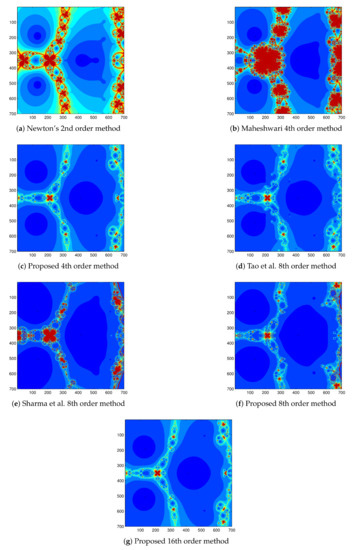
Figure 2.
Basin of attraction for , by different methods.
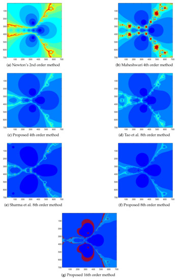
Figure 3.
Basin of attraction for , by different methods.
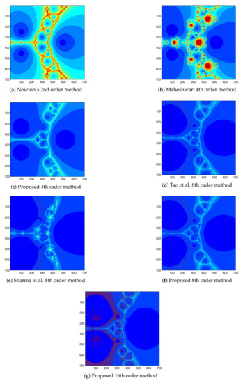
Figure 4.
Basin of attraction for , by different methods.
- The basins of attraction of all the methods contains Julia set with fractal boundaries and chaotic behavior with more or less concentration.
- The basins of attraction of second-order Newton’s method, the fourth-order Maheshwari method [4], looks similar, while that of remaining proposed method 4, 8, 16 order methods, method of Tao et al. [2], and method of Sharma et al. [16] appear to be the same.
- The basins of attraction of second-order Newton’s method, fourth-order Maheshwari method, and the fourth-order proposed method contains more number of orbits in comparison to the eighth and sixteenth order methods.
- Again, basins of attraction of the eighth and sixteenth order methods are darker than the second-order Newton’s method, fourth-order Maheshwari method, and fourth-order proposed method.
- Basins of attraction in Figure 1 show that the proposed fourth-order method is the best method for the test function as it contains less chaotic behavior. The proposed eighth-order method and method of Tao et al. are also good but having some chaotic behavior on the vertical edges.
- Basins of attraction in Figure 2 show that the proposed sixteenth-order method is the best method for the test function as it contains less fractal Julia set and less chaotic behavior with bigger orbits showing high speed of convergence to the roots. The proposed fourth-order method is also looking good.
- Basins of attraction in Figure 3 show that the proposed eighth-order method and method of Sharma et al. are the best methods for the test function as they are converging to the roots with eighth-order convergence having fewer fractal boundaries and chaotic behavior. The proposed fourth-order method and method of Tao et al. are also good methods.
- The proposed eighth-order method seems to be the best method for the test function as the basins of attraction contains less fractal boundaries and chaotic behavior (see Figure 4). Meanwhile, the proposed fourth-order method and eighth-order method of Tao et al. are also working well.
7.2. For Outer Functions and
We have also considered two outer functions for the illustrations of the dynamics of the iterative methods under the same previous conditions. We have plotted the fractal patterns graph of the functions and for the different iterative methods with a fixed different color to each zero of the basins of attraction:
From the fractal patterns of the different iterative methods in Figure 5 and Figure 6, the following results may be concluded:
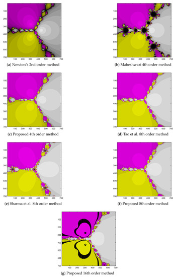
Figure 5.
Basin of attraction for , by different methods.
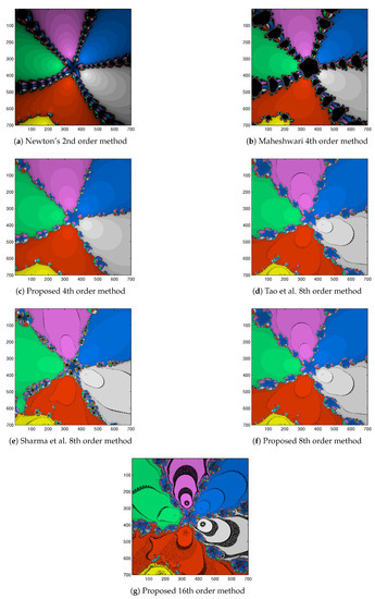
Figure 6.
Basin of attraction for , by different methods.
- The basin of attraction of all the methods contains the Julia set with fractal boundaries and chaotic behavior with more or less intensity.
- Basin of attraction of second-order Newton’s method, fourth-order Maheshwari method [4] looks similar, while that of the remaining proposed method 4, 8, 16 order methods, method of Tao et al. [2], and the method of Sharma et al. [16] appear to be the same.
- Basins of attraction of the second-order Newton’s method, fourth-order Maheshwari method, and fourth-order proposed method contain more orbits in comparison to the eighth-order methods.
- Basins of attraction in Figure 5 show that the proposed eighth-order method and Tao et al. eighth-order methods are the best methods for the test function , as it contains the less chaotic behavior with eighth-order convergence speed. The proposed fourth-order method and method of Sharma et al. are also good but have some fractal boundaries.
- Basins of attraction in Figure 6 show that the proposed fourth and eighth order method are the best method for the test function as it contains a less fractal Julia set and chaotic behavior with a high speed of convergence to the roots. The method of Sharma et al. and the method of Tao et al. are also looking good.
8. Future Work
Furthermore, we may consider the Juia set and Mendelbrot set related to our proposed methods. It will be interesting to see that what shape of figures of Julia sets and Mandelbrot sets comes out to be. We may follow the famous work of Mamta rani, and other authors who have considered the Julia sets and Mandelbrot sets in Noor orbit [8]. These proposed methods may allow us to study the Julia sets and Mandelbrot sets in a broader sense.
9. Conclusions
We obtained three new optimal order Newton’s-like methods for finding the root of the nonlinear equation . We have discussed the convergence analysis and dynamics of our methods. Numerical results reveal that the proposed 8th and 16th order optimal methods are more effective than the other methods at the point considered, as they are converging to the root with high speed. We have studied extraneous fixed points, and they are repulsive. From the fractal patterns graph, we observe that the basins of attraction of some selected examples are also supporting the numerical results; the proposed 8th order method is best here, but sometimes, a chaotic behavior can be seen with an increasing order of convergence. Hence, we conclude by the fractal patterns graph and table that the proposed 4th, 8th, and 16th order optimal methods are more productive than the existing order methods.
10. Patents
This section is not mandatory but may be added if there are patents resulting from the work reported in this manuscript.
Author Contributions
All authors have contributed to this work equally. All authors have read and agreed to the published version of the manuscript.
Funding
This research received no external funding.
Institutional Review Board Statement
Not applicable.
Informed Consent Statement
Not applicable.
Data Availability Statement
Not applicable.
Conflicts of Interest
The authors declare no conflict of interest.
Abbreviations
The following abbreviations are used in this manuscript:
| MDPI | Multidisciplinary Digital Publishing Institute |
| DOAJ | Directory of Open Access Journals |
| TLA | Three Letter Acronym |
| LD | Linear Dichroism |
References
- Singh, M.K.; Singh, A.K. Variant of Newton’s Method Using Simpson’s 3/8th Rule. Int. J. Appl. Comput. Math. 2020, 6, 20. [Google Scholar] [CrossRef]
- Tao, Y.; Madhu, K. Optimal Fourth, Eighth and Sixteenth Order Methods by Using Divided Difference Techniques and Their Basins of Attraction and Its Application. Mathematics 2019, 7, 322. [Google Scholar] [CrossRef]
- Singh, M.K. A Six-order variant of Newton’s method for solving non linear equations. Comput. Meth. Sci. Technol. 2009, 15, 185–193. [Google Scholar] [CrossRef]
- Maheshwari, A.K. A fourth-order iterative method for solving nonlinear equations. Appl. Math. Compt. 2009, 211, 383–391. [Google Scholar] [CrossRef]
- Kung, H.T.; Traub, J.F. Optimal order of one-point and multipoint iteration. J. Assoc. Comput. Mach. 1974, 21, 643–651. [Google Scholar] [CrossRef]
- Cordero, A.; Torregrosa, J.R.; Vasileva, M.P. A family of modified ostrowski’s methods with optimal eighth order of convergence. Appl. Math. Lett. 2011, 24, 2082–2086. [Google Scholar] [CrossRef]
- Sharma, R.; Bahl, A. Optimal Eighth Order Convergent Iteration Scheme Based on Lagrange Interpolation. Acta Math. Appl. Sin. Engl. Ser. 2017, 33, 1093–1102. [Google Scholar] [CrossRef]
- Ashish; Rani, M.; Chugh, R. Julia sets and Mandelbrot sets in Noor orbit. Appl. Math. Comput. 2014, 228, 615–631. [Google Scholar]
- Scott, M.; Neta, B.; Chun, C. Basin attractors for various methods. Appl. Math. Comput. 2011, 218, 2584–2599. [Google Scholar] [CrossRef]
- Ardelean, G. A comparison between iterative methods by using the basins of attraction. Appl. Math. Comput. 2011, 218, 88–95. [Google Scholar] [CrossRef]
- Traub, J.F. Iterative Methods for the Solution of Equations; Prentice Hall: Clifford, NJ, USA, 1964. [Google Scholar]
- Ortega, J.; Rheinholdt, W. Iterative Solution of Nonlinear Equations in Several Variables; Academic Press: New York, NY, USA, 1970. [Google Scholar]
- Petkovic, M.S.; Neta, B.; Petkovic, L.D.; Dzunic, J. Multipoint Methods for Solving Nonlinear Equations; Elsevier: Amsterdam, The Netherlands, 2012. [Google Scholar]
- Amat, S.; Busquier, S.; Plaza, S. Review of some iterative root-finding methods from a dynamical point of view. Scientia 2004, 10, 3–35. [Google Scholar]
- Mandelbrot, B.B. The Fractal Geometry of Nature; Macmillan: New York, NY, USA, 1983; ISBN 978-0-7167-1186-5. [Google Scholar]
- Sharma, J.R.; Arora, H. An efficient family of weighted-Newton methods with optimal eighth order convergence. Appl. Math. Lett. 2014, 29, 1–6. [Google Scholar] [CrossRef]
- Bradie, B. A Friendly Introduction to Numerical Analysis; Pearson Education Inc.: New Delhi, India, 2006. [Google Scholar]
- Vrscay, E.R.; Gilbert, W.J. Extraneous fixed points, basin boundaries and chaotic dynamics for Schroder and Konig rational iteration functions. Numer. Math. 1987, 52, 1–16. [Google Scholar] [CrossRef]
- Julia, G. Memoire sure l’iteration des fonction rationelles. J. Math. Pures Et Appl. 1918, 81, 47–235. [Google Scholar]
- Yoneyama, K. Theory of continuous sets of points. Tohoku Math. 1917, 12, 43–158. [Google Scholar]
- Argyros, I.K.; Magrenan, A.A. Iterative Methods and Their Dynamics with Applications: A Contemporary Study; CRC Press: Boca Raton, FL, USA; Taylor and Francis: Boca Raton, FL, USA, 2017. [Google Scholar]
Publisher’s Note: MDPI stays neutral with regard to jurisdictional claims in published maps and institutional affiliations. |
© 2021 by the authors. Licensee MDPI, Basel, Switzerland. This article is an open access article distributed under the terms and conditions of the Creative Commons Attribution (CC BY) license (http://creativecommons.org/licenses/by/4.0/).